The Effects of Sound Speed Profile to the Convergence Zone in Deep Water

Abstract

The structure of a sound speed profile (SSP) in deep water causes refraction of sound rays and Convergence Zones (CZs) of high intensity where the rays focus at shallow depth. Study of sound field characteristics in the CZs has always been the focus of deep-water acoustics research. Many studies have been conducted on sound propagation in different parts of the oceans with different environments and, in this paper, the range and width of CZ is analyzed in the East Indian Ocean (EIO) and the South China Sea (SCS). Through the experimental data collected in different seasons with the propagation conditions change in the EIO and the SCS, we observe that the SSPs in different marine environments have a significant impact on the CZs of deep water. The sound channel mixing layer and isothermal layer have great effect on the CZ ranges. The water depths in the two experimental areas are similar, the range of the first CZ in the EIO is 7–8 km farther than that in the SCS, and the width of the CZs in the EIO is about 2–3 km narrower than that in the SCS. The surface mixed layer and the thermocline affect the CZ width but has little effect on the CZ range when the sound speed at the source and the bottom are practically the same. As the propagation conditions change along the seasons in the EIO, the range of the first CZ is almost the same, but the width of the CZs in the summer is about 2 km narrower than that in the spring. The water depth affects the CZ width but has little effect on the CZ range if the CZs can be formed. The different CZ characteristics between EIO and SCS are explained by both theoretical calculation and numerical simulation. The influence of the SSP structure and water depth on the CZ range are analyzed and the corresponding mechanism is explained. The research results are of great significance for underwater acoustic detection in deep sea.

1. Introduction

The formation of convergence zones (CZs) is a unique phenomenon in deep-water sound propagation, which is different from sound propagation in shallow water. The transmission loss (TL) difference inside the CZ and shadow zone can reach 10–20 dB [1]. Using the properties of the CZs are beneficial to target detection and long-range communication in deep water. Therefore, the CZ study has been given much more attention since World War II [2,3,4].

Extensive research has been carried out previously on communication and characteristics of deep-water CZ and reported in many papers [5,6,7]. Research has also been done on investigating travel time and phase fluctuations induced by the sound-speed variations resulting from temperature fluctuations inherent in long-range CZ propagation. Stephen and John observed how the sound speed profile structures that affect the travel time arrive early in the North Pacific at low and middle frequencies [8,9]. Beilis et al. [10] and Bongiovanni et al. [11] have forecast the range of CZ based on the fluctuation equation, and more factors are taken into account, resulting in more complex expressions, which are not conducive to practical use. A convergence-zone-range slide rule (TACAID 6–10) was developed in 1973 by the Naval Underwater Systems Center based on an analysis of oceanographic data performed by E.M. Podeszwa, but this slide rule could only be used in the North Atlantic and North Pacific oceans, and the Mediterranean, Norwegian, and Caribbean seas to determine CZ ranges [12]. In the North Atlantic Ocean, CZs are seen to appear at intervals of approximately 65 km. During an experiment in the northern Philippine Sea in 2009, Baggeroer [6] found that the range of the CZ is about 60 km, based on the observed experimental data. In domestic research, Zhang et al. [13] analyzed the CZ characteristics and the calculation method for the CZ range and width based on the WKBZ theory, showing that the width of CZ increases with the increase of range. Zhang et al. [14,15] and Cheng et al. [16] quantitatively analyzed the influence of the thermocline change on the CZ range through simulation data, concluding that the increase of surface sound speed puts the CZ farther from the source. Fan et al. [17] carried out the characteristic analysis and CZ calculation, and statistically analyzed the relationship between the CZ range and the parameters of the surface sound speed, depth of sound channel axis, and water depth, concluding that the CZ range is closely related to these parameters. Lin et al. [18] analyzed the effect of CZ on sonar detection performance by simulation data in deep sea and a quantitative performance evaluation model was constructed that evaluates the sonar detection ability. The authors showed that if there are no CZ sound propagation conditions, the detection of sonar will be greatly reduced. Li et al. [19,20] analyzed the characteristics of sound propagation in complex deep-water environment and the vertical correlations in the first CZ through the South China Sea (SCS) experiment, concluding that the vertical correlation coefficient in the CZ is higher than that in the shadow zone. Piao et al. [21] analyzed the characteristics and formation mechanism of the CZ below the sound channel axis in the incomplete deep channel in the SCS, and using long range experimental data to verify the CZ ranges and width. However, most present studies on deep-water CZ in China are mainly focused on the SCS. There is little work on sound propagation in the East Indian Ocean (EIO). The EIO is an important sea area of the world, and because of its special environmental characteristics, which significantly affect underwater acoustic propagation, it is an interesting case to better understand the dynamics of CZ formation.

In this paper, the sound propagation data from the EIO and the SCS are used to analyze the impact of sound channels and propagation conditions change along different seasons on the deep-water CZs. In the EIO, CZs are seen to appear at intervals of approximately 58 km, compared to around 50 km in the SCS. Through the experimental data, we have identified the changes in sound channel refraction and the resulting shifts in focusing CZ ranges and found that the changes in surface sound speed makes little effect on CZ ranges. At the same time, the CZ range and width have been analyzed extensively both through theoretical or numerical investigation and through sound propagation experiments.

2. Methods and Experiment Introduction

2.1. Experiments Observation in the EIO and SCS

In August 2019, a sound propagation experiment was performed in the deep-water area of the EIO (Figure 1 Area I). This is the first Chinese acoustic propagation investigation experiment in the EIO. The objective was to explore how sound propagation changes when the oceanographic conditions changes along with the seasons. Two years later, in March 2021, a sound propagation experiment was performed along the same propagation track in Area I. In the experiments, we found that the SSP of the EIO are very different from the previous measurement in the SCS.

The experimental layout is shown in Figure 2. The vertical line array (VLA) is composed of multiple hydrophones covering the full water depth (100 m to 3600 m), but the VLA design is not exactly the same in these experiments. In other words, the depths of the receivers are not exactly the same in each experiment. The sensitivity for each hydrophone is −170 dB (reference level is 1 V/μPa). The sampling rate of the hydrophones is 16 kHz. The wide band signals (WBS) were recorded from 1 kg TNT dropped from the R/V Shi Yan 1 from the Institute of Acoustics, Chinese Academy of Sciences along the propagation tracks. The nominal detonation depth of the TNT charges is 200 m. The ocean bottom is nearly flat and the average depth is about 3700 m within 130 km of each propagation track.

In addition, we also conducted a similar acoustic propagation experiment in the SCS in April 2018 (Figure 1 Area II). In order to analyze and compare the similarities and differences of the sound propagation laws for the two experiments, we choose a sound propagation track with relatively flat seabed topography in the SCS. The water depth of the propagation track in the SCS is similar to that of the EIO. The comparisons of the water depth and sound speed profile (SSP) for the three experiments are shown in Figure 3. The water depths of the EIO and SCS experiments are 3500 m and 3700 m, respectively, which are basically the same. The bathymetry is generally flat for each track. Figure 4 shows the SSP change with distance obtained by the Expendable Bathy Thermographs (XBTs) and Conductivity-Temperature-Depth (CTDs) on the propagation paths in the experimental period. The XBT intervals are 10 km along the track. It can be seen that the SSPs change slowly on the propagation path. In short-distance sound propagation, this slow change has little effect on the result analysis. In the following analysis, we consider that the SSP is range-independent.

As shown in Figure 3 and Figure 4, the sea-surface sound speed in the EIO is higher than that in the SCS, and the sound speed changes more drastically above 200 m depth. The SSP in the EIO is slowly varying within a large depth change from 500 m to 2000 m. The sound speed value is close to the minimum in these depths. There is an extensive constant sound speed layer in the channel. This shows that the sound channel axis in the EIO is not well defined. The minimum sound speed is 1491 m/s at the depth of 1800 m. The channel axis in the SCS is approximately at the depth of 1100 m, and the minimum sound speed is 1484 m/s. In the EIO and SCS experiments, the sound speed at the sea surface is greater than that near the seabed, which is a typical deep-water incomplete channel.

2.2. Methods for Data Analysis

In the experiment, the acoustic signal received by the hydrophone is recorded as $x\left(t\right)$, and the Fourier transform of $x\left(t\right)$ as $X_i$. Then we obtain acoustic signal energy with the bandwidth of $\Delta f$ within 1/3-octave bandwidth corresponding to center frequency $f_0$.

$$E\left(f_0\right)=\frac{2}{F_s^2}\frac{1}{n{f}_2-n{f}_1+1}{\displaystyle \sum }_{i=n{f}_1}^{n{f}_2}{\left|X_i\right|}^2$$

(1)

where $F_s$ is the sampling rate, and $n{f}_1$ and $n{f}_2$ represent the upper and lower frequencies, respectively, of the band with center frequency $f_0$.

Then, we obtain the $TL$:

$$TL\left(f_0\right)=SL\left(f_0\right)-\left(10\log \left[E\left(f_0\right)\right]-b\right)$$

(2)

where b is the sensitivity of hydrophones. All quantities in Equation (2) are in dB. $SL\left(f_0\right)$ is the source level we have measured in the previous experiment; the methods of source level calibration are shown in Ref. [22].

In this experiment, the SL was measured, and it can be considered as a constant and different at each central frequency. To reduce accidental errors, eight TNT charges at 200 m, which were the same as were used in the previous experiment, were used in this experiment. One of the received WBS is shown by black curves in Figure 5a. During data processing, only the energy of the direct sound wave is calculated, and the reflected wave by the sea surface is set to zero, such as the red curve in Figure 5a. We calculated the SL by the processed WBS. The source level for the central frequency of 50–2000 Hz (interval 50 Hz) is shown in Figure 5b. The bandwidth was one-third octave for the central frequencies range 50–1000 Hz, and the central frequencies range 1000–2000 Hz is calculated using the 200 Hz bandwidth. The eight black curves are the value of each wide band signal, the red curve is the average value, which was also the value we used.

2.3. Sound Propagation Data Analysis

Due to the design of VLA, there is a receiver from the VLA, which has the same depths of 255 m in the EIO 2019 and SCS 2018 experiments. The near-receiving depth in the EIO 2021 experiment is 285 m. The experimental TLs from the two receivers shown as red dots in Figure 6. The central frequency of the source is 300 Hz, and the source depth is 200 m. To analyze the experimental results, a sound field model RAM [23] based on the parabolic equation theory is used to calculate the TLs of the two survey tracks with the same receiver depth. The numerical results are shown as blue lines in Figure 6, which agrees very well with experimental data shown as the red solid dots. In the simulations, we are assuming a half space geo-acoustic model for the ocean bottom. The bottom acoustic parameters of the EIO are a sound speed of 1585 m/s, density of 1.7 g/cm³, and absorption coefficient of 0.15 $\mathrm{dB}/\mathsf{\lambda }$; the bottom acoustic parameters of the SCS are a sound speed of 1555 m/s, density of 1.7 g/cm³, and absorption coefficient of 0.15 $\mathrm{dB}/\mathsf{\lambda }$ [24].

Comparing the experimental data in Figure 6, we observe that the propagation paths cover two CZs, and the first CZ ranges in the EIO and SCS are about 58 km and 50 km at the same receiving depth, respectively. The first CZ range in the EIO is 7–8 km farther than that in the SCS, and the CZ width of the EIO is narrower than 2–3 km that in the SCS. Next, we will explain the reasons for this phenomenon in these experiments.

3. Results and Discussion

3.1. The Conditions of Forming the CZ

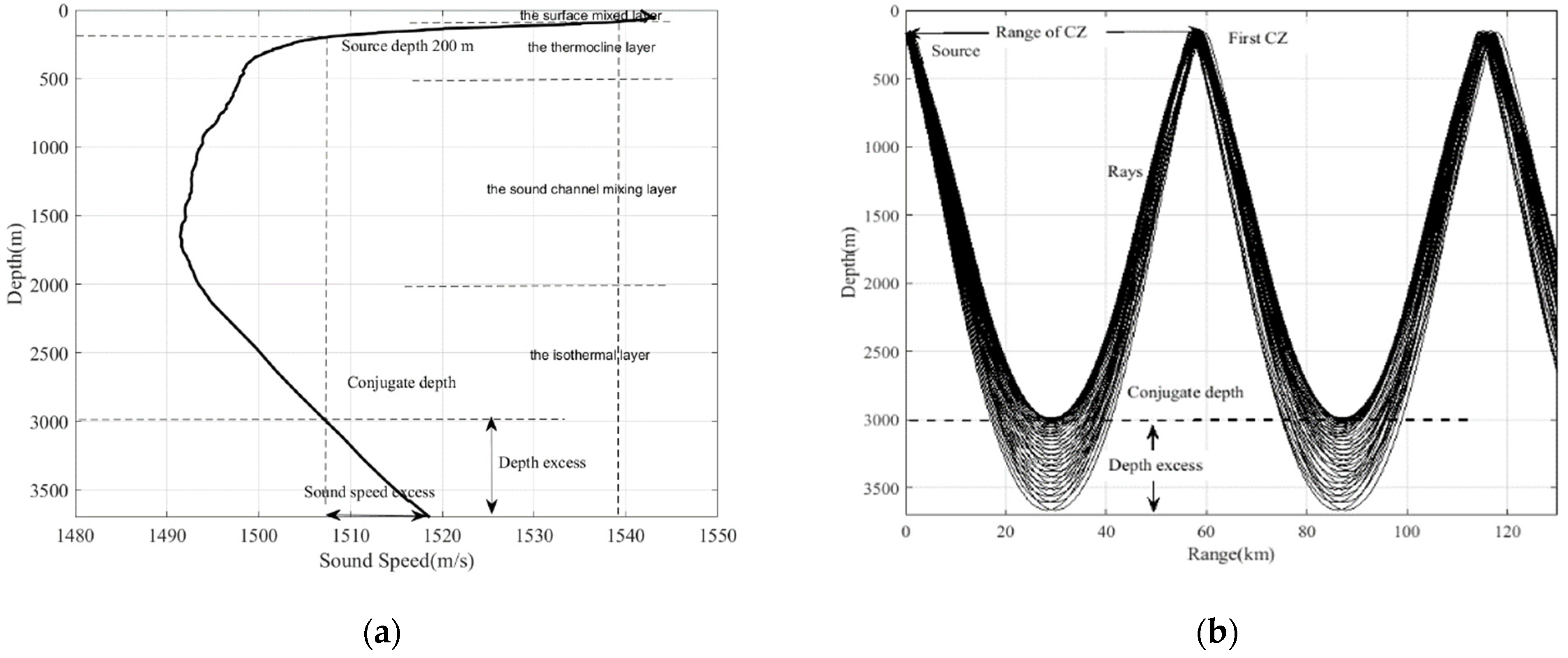
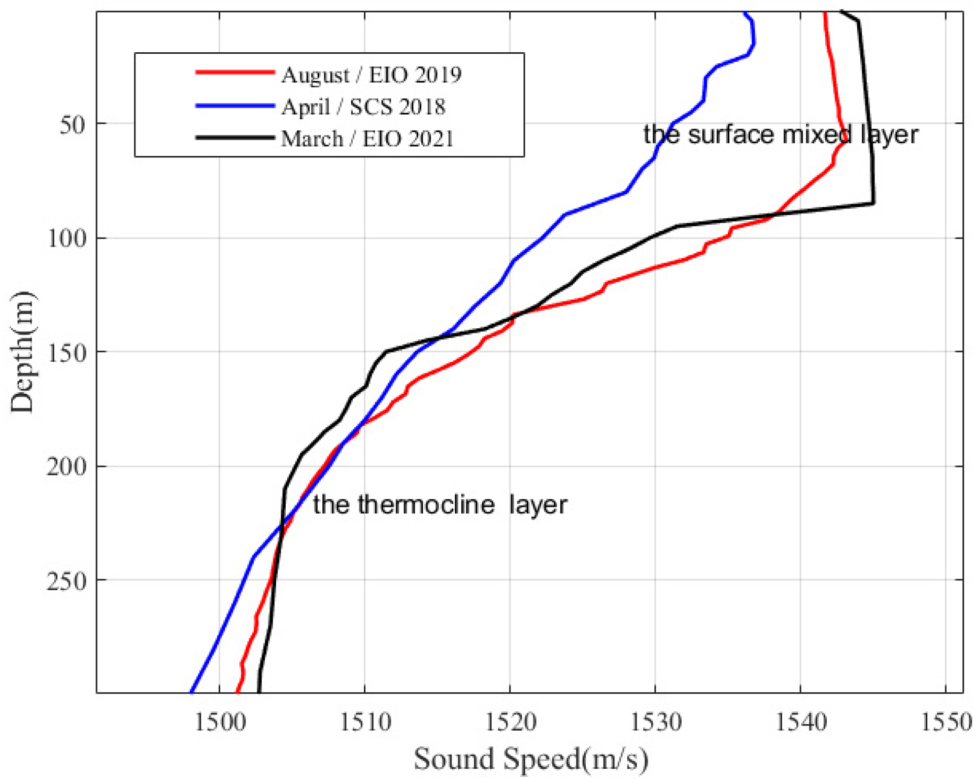
The vertical temperature structures of the ocean can, in general, be divided into four layers as shown in Figure 7a: the surface mixed layer, the thermocline, the sound channel mixing layer, and the isothermal layer with weak vertical temperature gradient. The depth where the sound speed is equal to that at the sound source is called the conjugate depth or critical depth. The region below the conjugate depth to the bottom is called the depth excess, and the difference between the sound speed at the conjugate depth to the bottom is called the sound speed excess. The range of CZ refers to the location of the sound source to the first sound rays inversion convergence to the sea surface, as shown in Figure 7b.

When a source is close to the surface, according to the Snell law, the sound rays bend toward the vertical. In other words, the sound rays emitted by the source will bend to the bottom. The sound rays will gradually bend toward the surface after passing through the sound channel axis where the sound speed is minimum, where sound speed increases with depth in the deep isothermal layer because of the increase in pressure. When the sound speed near the bottom is greater than that close to the source, some sound rays with small grazing angles do not touch the bottom and reverse upward near conjugate depth. After this process, sound rays converge at the surface to form a CZ.

To form a CZ, both the sound source and receiver should be placed in the sound channel, and the water depth should be great enough to reach the conjugate depth. If there is a depth excess in the deep-water waveguide, some deep refracted sound rays do not touch the ocean bottom. These rays are refracted upward to the sea surface and are focused together to form a CZ close to the surface.

The sound speed is determined largely by the water temperature. Thus, water temperature near the sea surface and the water depth in any particular area will largely determine whether sufficient depth excess exists and therefore whether a CZ will occur. Charts of surface temperature and water depth can then be used as basic prediction tools for ascertaining the existence of CZs.

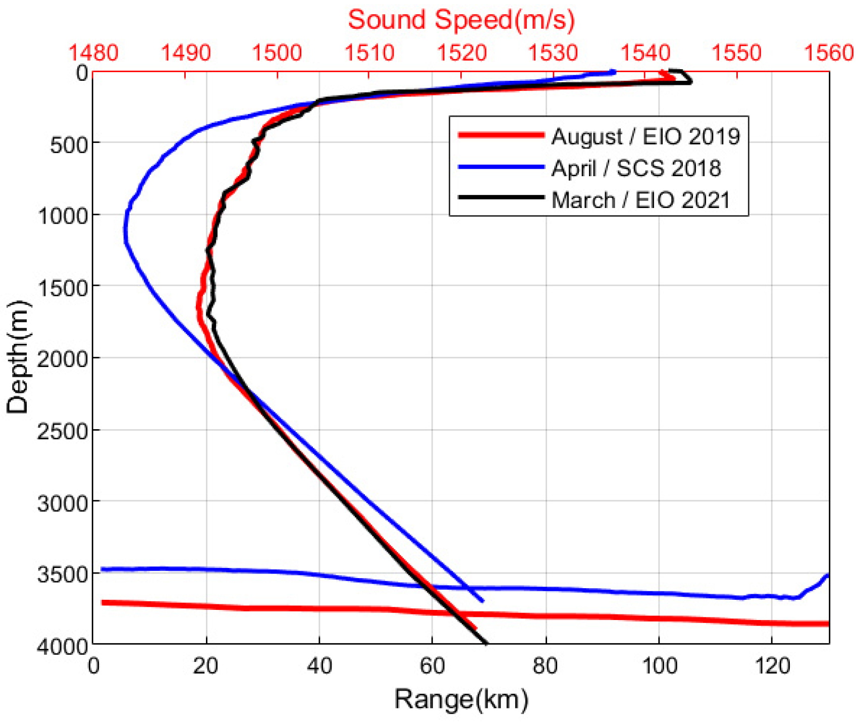
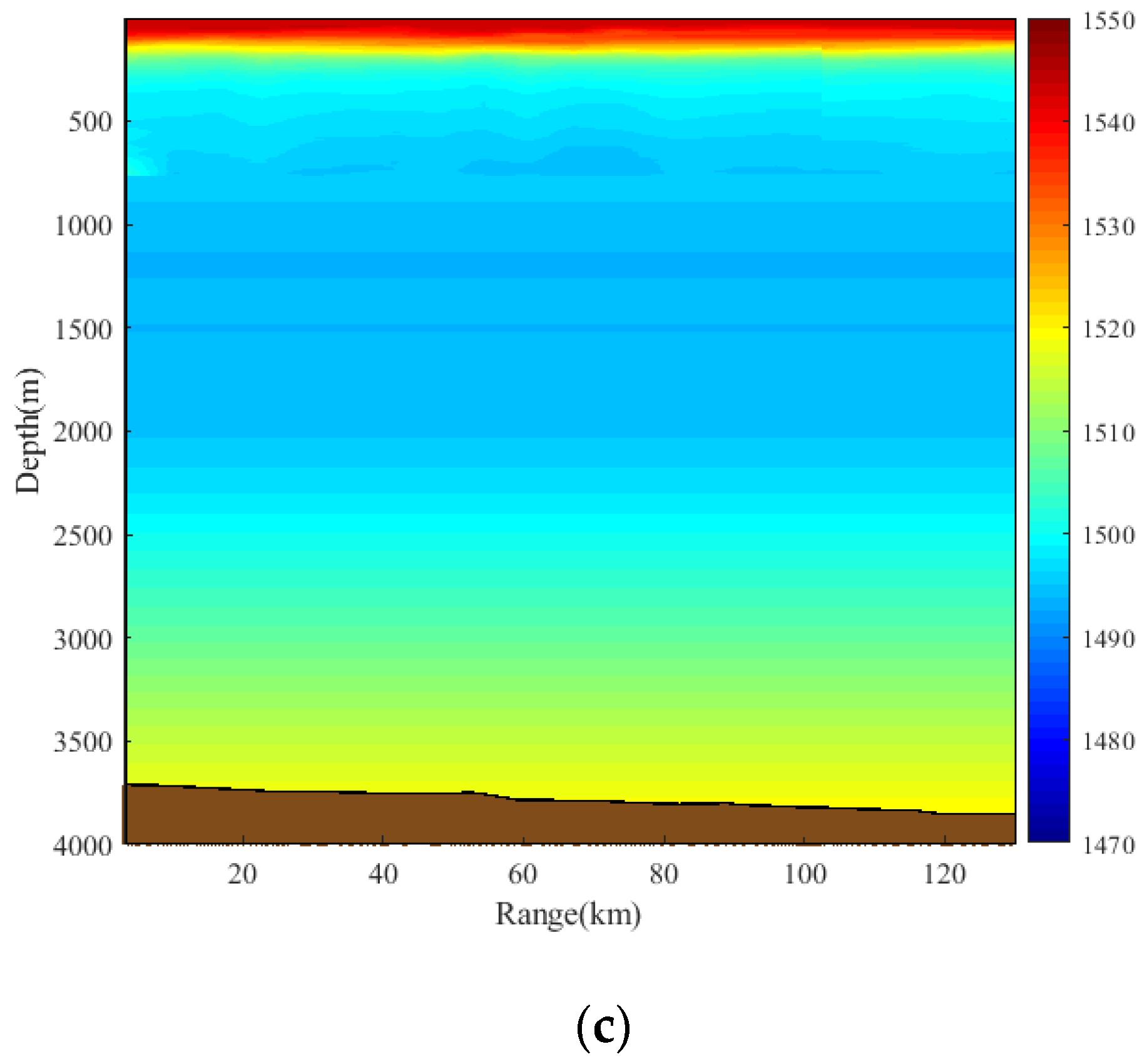
As seen in the sound speed profiles in these two ocean areas shown in Figure 3, the sound speed at the source is less than that at the bottom, so CZs will occur in both the EIO and SCS.

3.2. The Theoretical Analysis on the CZ Range

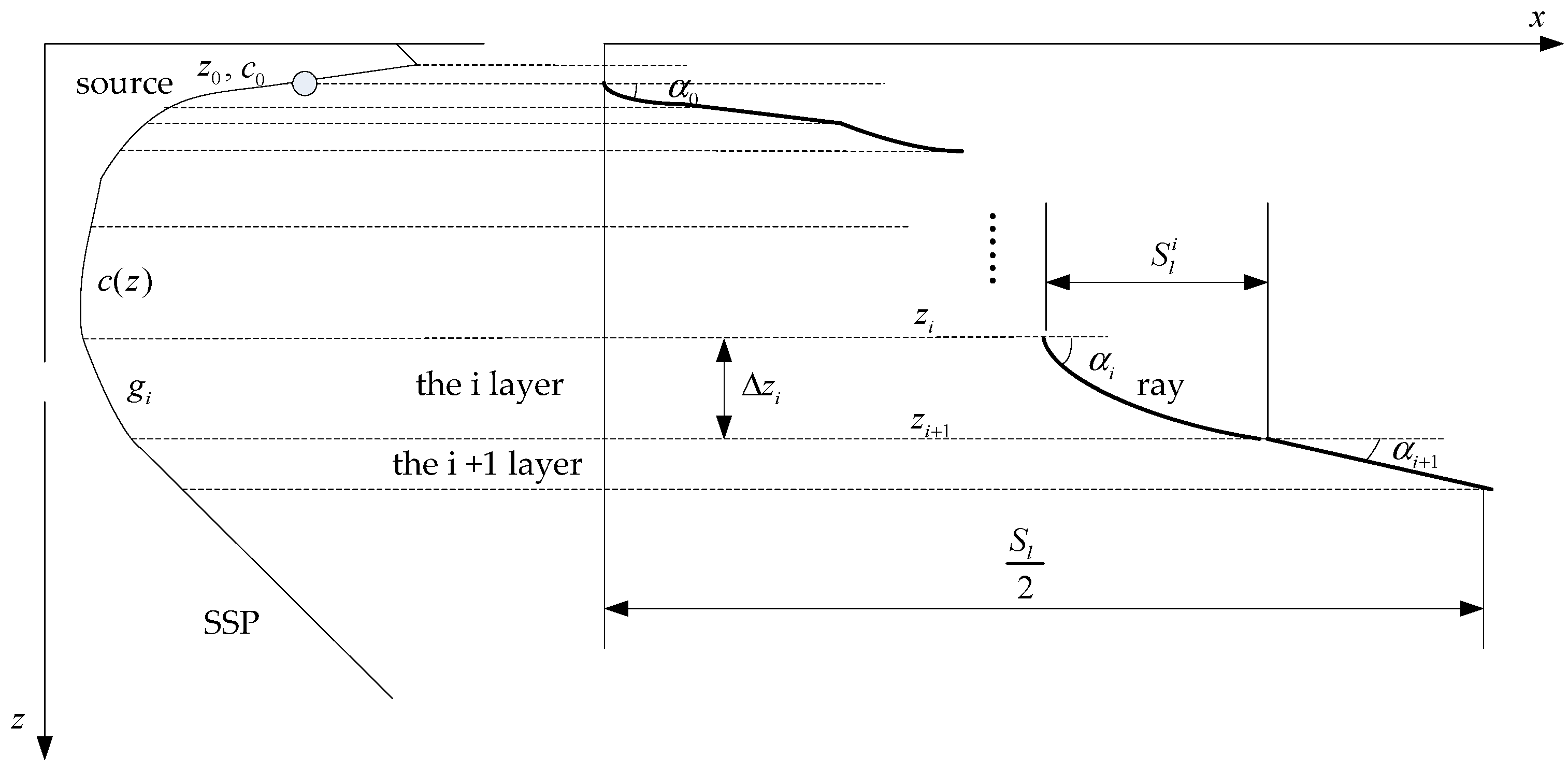
To explain the effects of the sound speed profile structure on the CZ range, we use the numerical calculation to predict the CZ range in the underwater environment. As we know, the sound speed profile can be described as the function of the depth. The linearization of the sound speed profile to obtain the horizontal range of sound ray has been widely used [1]. We analyzed the CZ range by calculating the horizontal range, and the linearized sound speed profile and the sound rays are shown in Figure 8.

For linear layered media, the horizontal distance of the sound ray through each sound speed layer is defined as the horizontal range$S_l^i$, which can be expressed by the wave number, and its expression [13] is:

$$S_l=2{\displaystyle \sum }_{i=1}^N{S}_l^i={\displaystyle \sum }_{i=1}^N{{\displaystyle \int }}_{z_i}^{z_{i+1}}\frac{2{\mu }_l}{\sqrt{k^2\left(z\right)-{\mu }_l^2}}dz$$

(3)

where N is the number of the layered media, $z_i$ and $z_{i+1}$ are the top and bottom depths of the layer I, respectively, $k\left(z\right)$ is wave number at the depth $z$, and ${\mu }_l$ is horizontal wave number.

The analytical solution of the horizontal range through a linear layered medium in Ref. [5] is:

$$S_l=\frac{c_0\left(z_0\right)}{cos\alpha \left(z_0\right)}{\displaystyle \sum }_{i=0}^{N-1}\left|\frac{sin{\alpha }_{i+1}-sin{\alpha }_i}{g_i}\right|$$

(4)

where $\alpha \left(z_0\right)$ and $c_0\left(z_0\right)$ are the sound ray initial grazing angle and sound speed at the source depth of $z_0$, respectively. $g_i$ is sound velocity gradient of the layer i, ${\alpha }_i$ and ${\alpha }_{i+1}$ the sound ray grazing angles at the $z_i$ and $z_{i+1}$ depths, respectively.

With the theoretical expression of the horizontal range, the CZ range can be obtained with higher accuracy from the given source depth and the known hydrological conditions of sound propagation. The calculation of the CZ range can be simplified as the horizontal range of the sound ray with a grazing angle of 0° nearest the bottom. This sound ray has the maximum reversal depth.

During the experiment, the SSP was acquired from measurements based on time or space sampling. The accuracy of the vertical distribution is sufficient to reflect the characteristics of the actual continuous SSP. The segmented broken line is used to replace the actual continuous SSP. This linear approximation method of sound speed is relatively simple and has been widely used [1]. In the following, the SSPs actually measured in the experiments will be segmented, and the theoretical estimation of the CZ range in the two environments will be carried out through iterative calculation according to Equation (4).

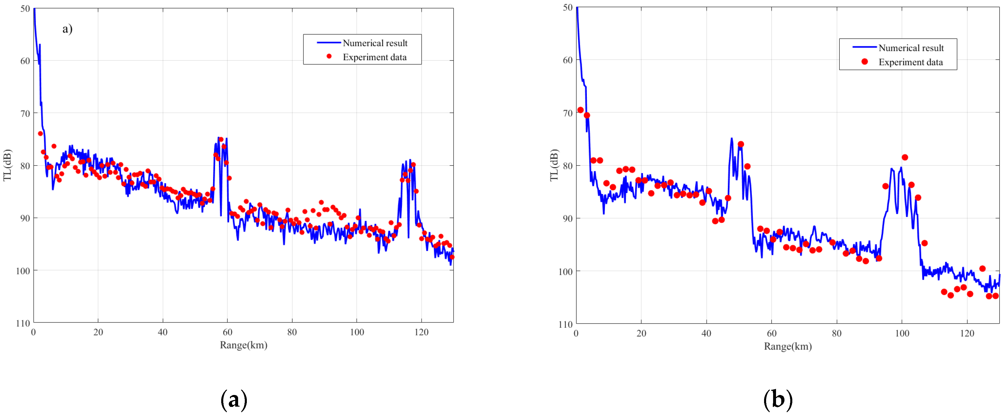
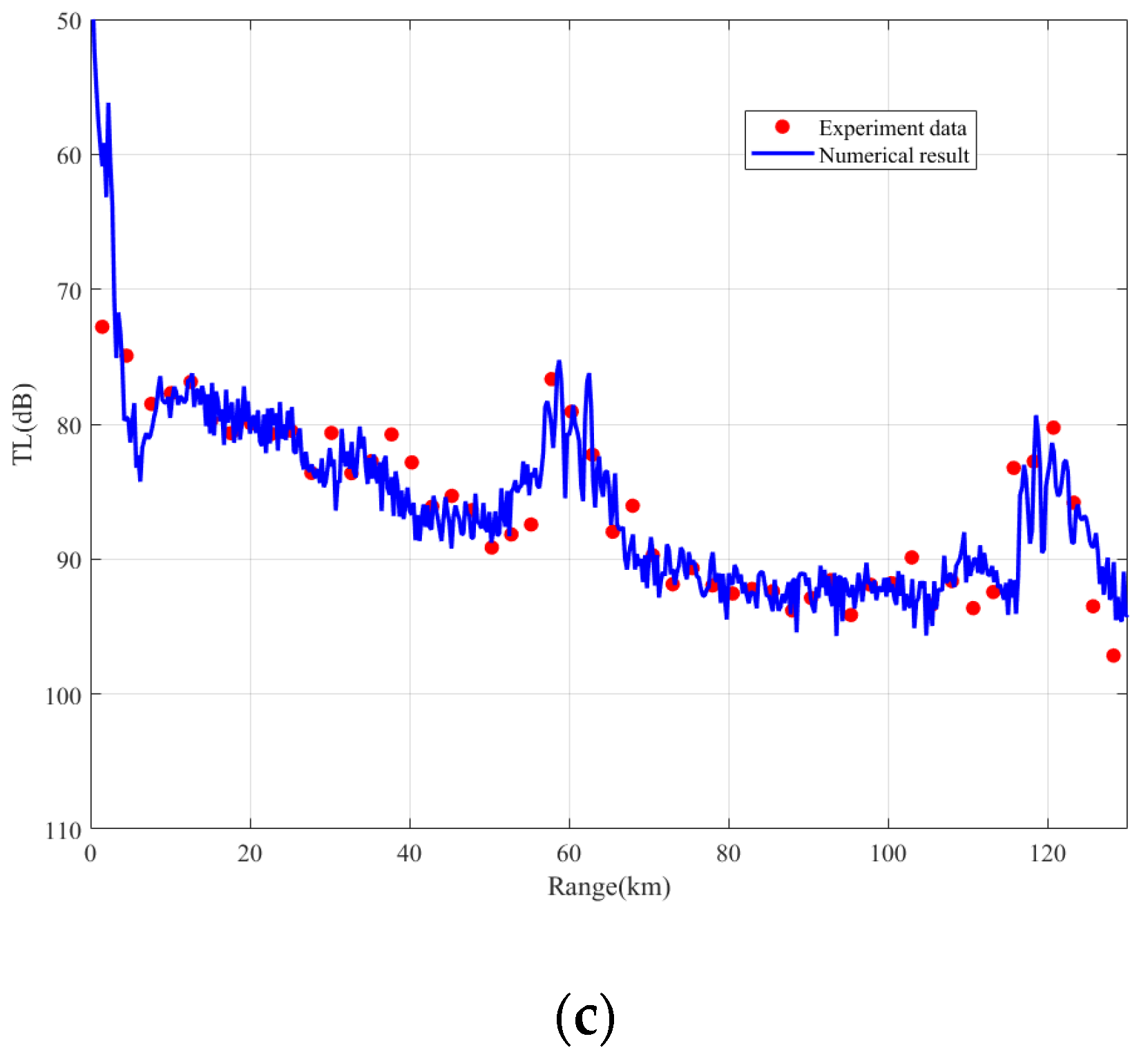
As defined above, the range of the sound ray with a grazing angle of 0° on the seabed is the first CZ range. According to the Snell law, the exit angle at the source is 6.9° for the ray with a grazing angle of 0° at the seabed in the EIO 2019. Similarly, the exit angle of this ray is 8.5° in the SCS 2018 and that of 7.5°in the EIO 2021. Substituting the exit angles into Equation (4), we get that the first CZ ranges in the EIO 2019, EIO 2021, and SCS 2018 are 58.6 km, 61.1 km, and 49.3 km, respectively, using a software of Matlab simulation calculation. The result is basically consistent with the CZ range obtained from the experimental data of the two sea areas shown in Figure 6.

From the theoretical analytical Equation (4) of the horizontal distance of the sound ray, it can be seen that the horizontal range of the sound ray is related to the source depth and the initial grazing angle. However, $\frac{c_0\left(z_0\right)}{cos\alpha \left(z_0\right)}$ is constant. Therefore, the CZ range is mainly related to the sound speed gradient $g_i$, which is the characteristics of the SSP structure.

3.3. Numerical Simulation and Analysis the CZ Phenomenon of the Two Sea Areas

Based on the standard model of SSP, Zhang et al. [14] analyzed the influence of some special environmental parameters on the convergence area, including the thermocline, mixed channel layer, isothermal layer, and sound channel axis. However, the actual changes of SSP in the ocean are complex and cannot be represented by simple changes in model parameters. Moreover, the SSPs from different areas may have great differences and cannot be described by the same model. According to the comparison of the hydrological environment of the EIO and SCS as shown in Figure 3, the difference of the SSPs from the two sea areas is the main reason why the CZ range of the EIO is farther than that in the SCS. At the same time, the SSPs from the same sea areas but in different seasons may affect the convergence zone ranges and widths.

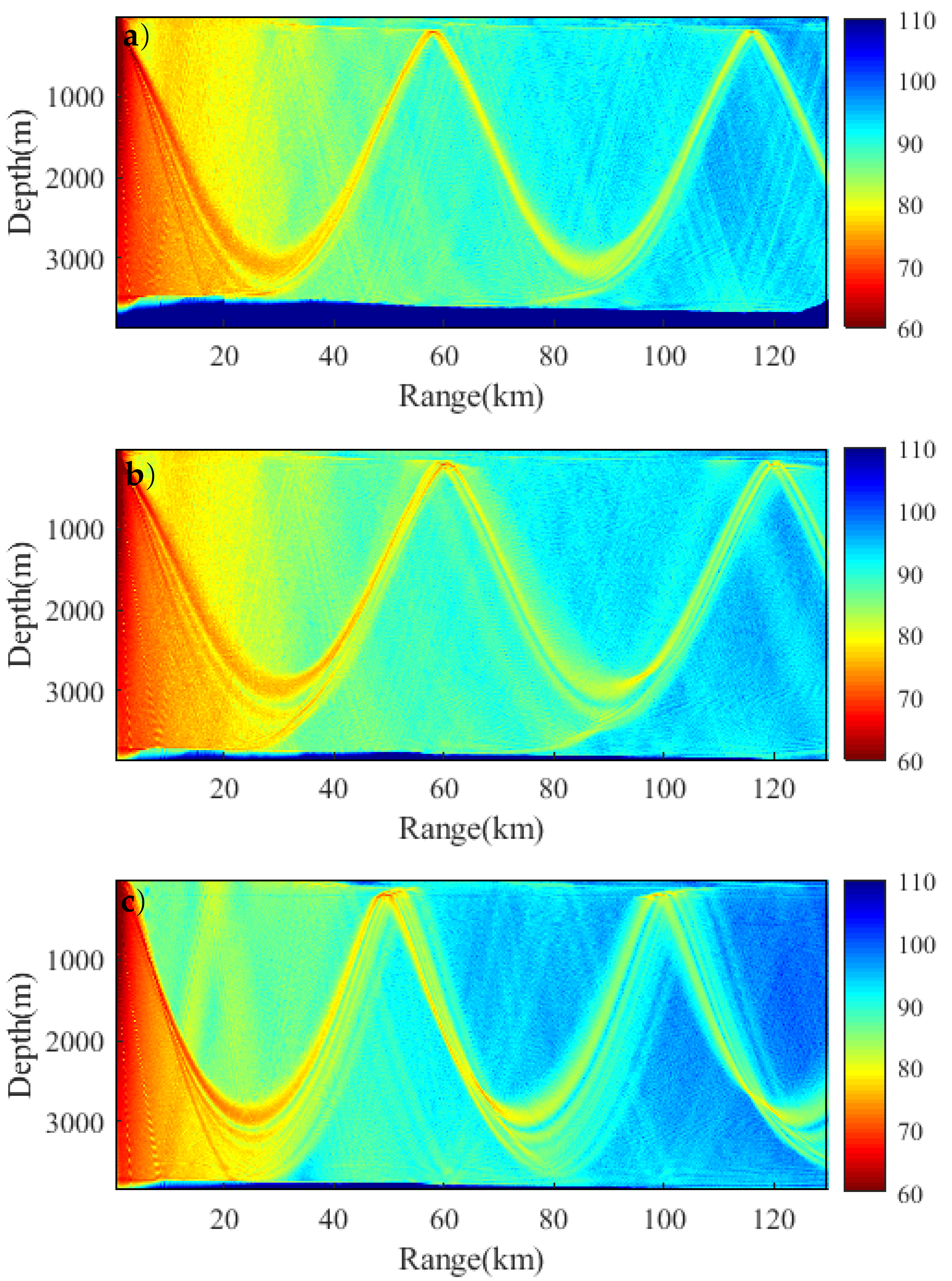
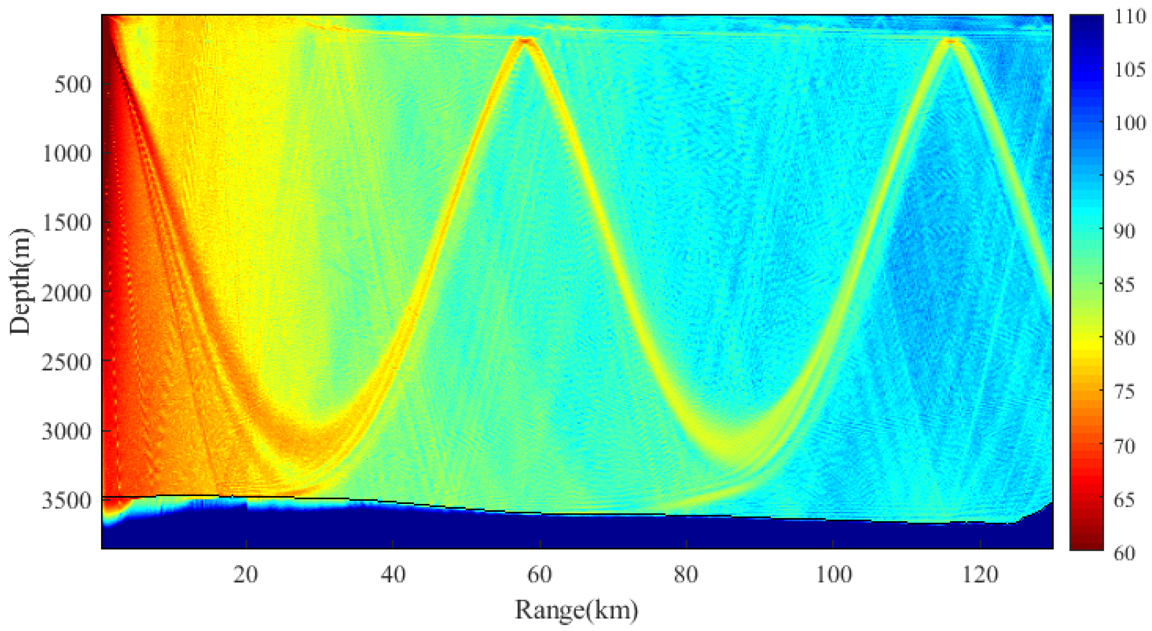
Figure 9 gives the simulated TLs using the environmental parameters measured in three experiments by the RAM-PE model, in which source depth is 200 m, and the central frequency is 300 Hz. We can observe that the range and width of the CZ vary in different environments. To illustrate the problem, we choose the same conditions of sound propagation in the model simulation, in which source depth is 200 m, central frequency is 300 Hz, and receiver depth is 255 m. The result is shown in Figure 10.

From Figure 9 and Figure 10, we observe that the range and width of the first CZ in the EIO is 7–8 km farther and about 2–3 km narrower than that in the SCS at the same receiving depth. When the propagation conditions change within seasons in the EIO, the range of the first CZ is almost the same but slightly greater, but the width of the CZs in the summer is narrower by about 2 km than in the spring.

First, we will explain the reasons for the different CZ ranges and widths in two sea areas. Then, we will explain the reasons for this phenomenon of condition change within seasons in the EIO.

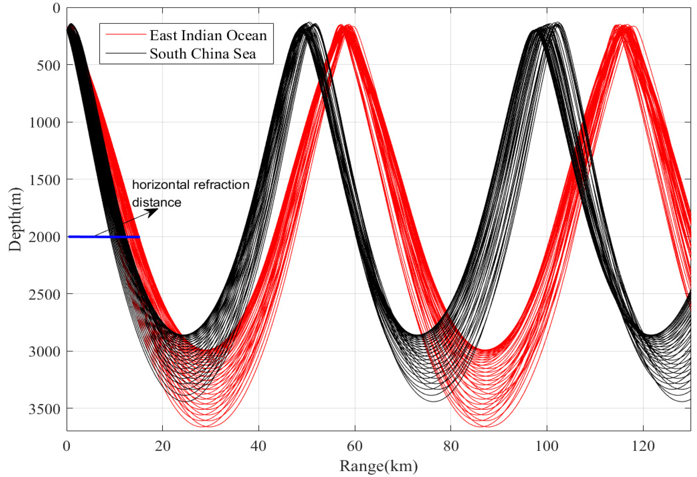
To explain the difference of CZ ranges between the EIO and SCS, the corresponding sound rays in these two sea areas are calculated by the Bellhop ray model [25], as shown in Figure 11.

From Figure 11, we observe that the first CZ ranges in the EIO (about 58 km) and SCS (about 50 km) are basically consistent with the CZ range calculated using the experimental data of the two areas. We can also observe that sound ray refraction is strong in the near field in the EIO because of the greater change of sound speed in the shallow depths. At the same time, the strong refraction causes sound rays to enter the sound channel mixing layer with different grazing angles. As shown in Figure 11, between 1000 m and 2000 m depth, the rays have a smaller grazing angle in the EIO relative to that in the SCS. As shown in Figure 9 and Figure 11, at the depth of 2000 m, the horizontal refraction distance (indicated by the blue line in the Figure 11) of the EIO is 15 km, and the distance is 11 km in the SCS. That is because of the relatively slow change of sound speed in the mixed channel layer of the EIO. There is an extensive constant sound speed layer in the channel. In this channel, the sound rays propagate along approximately a straight line in the EIO and the sound rays bends upward when they cross the sound channel axis in the SCS. So the horizontal refraction distance in the EIO is larger than that in the SCS. In addition, the grazing angles of the sound rays are also smaller when they enter the isothermal layer. A smaller grazing angle results in a greater horizontal refraction distance when the rays pass through the approximate depth excess. At the same time, the gradient of sound speed in the deep-water isothermal layer of the EIO is smaller than that of the SCS. It can be seen from the horizontal range of the sound ray in Equation (4) that the smaller the gradient $g_i$ of the sound speed, the less refraction of the sound rays, and the greater the horizontal range will be. This is also one of the reasons why the CZ in the EIO is farther away from the source.

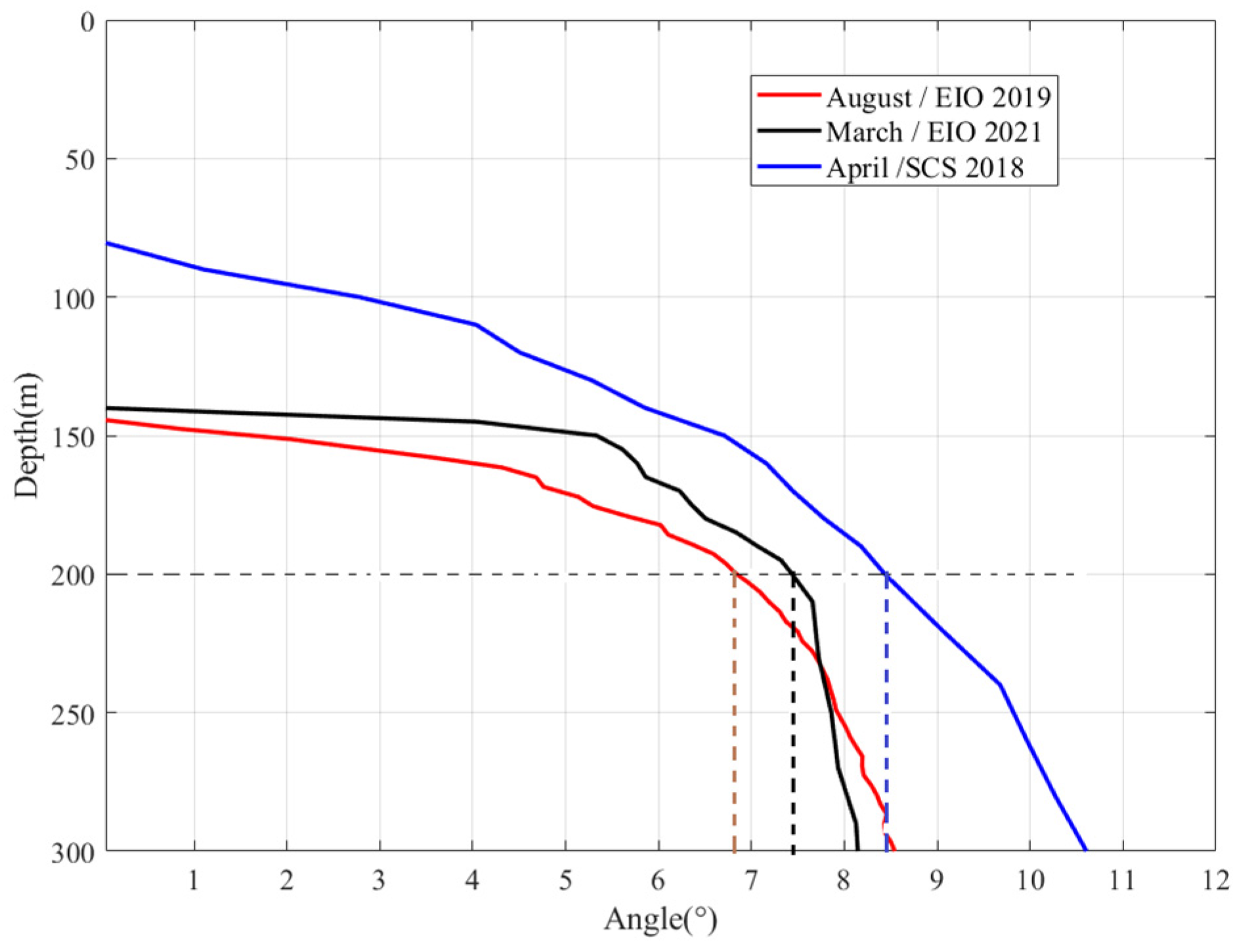
The sound ray with a grazing angle of 0° at the ocean bottom does not come into contact with the bottom. This ray is dominant to form a CZ at the sea surface. According to the Snell law, the emission angle of the sound ray at the source is:

$$cos\alpha =c\left(z_s\right)/c\left(\mathrm{D}\right)$$

(5)

where $c$($z_s$) is the sound speed in water at the source depth, c(D) is the sound speed in water at the bottom depth. When the grazing angle $\alpha$ at the source meets the condition $\alpha \le \mathit{arccos}(c$($z_s$)/c(D)), the sound rays would converge and, at this time, have a grazing angle of 0° at the ocean bottom.

c(D) is known, and $c$($z_s$) varies with the depth of the sound source $z_s$. Under the preconditions Equation (5) of the CZ formation, from the detailed sound speed, we get the curve of the source depth $z_s$ with the maximum emission angle $\alpha$ of a ray refracting at the bottom, as shown in Figure 12.

It can be deduced that when the source depth is 200 m, some emitted sound rays do not touch the bottom and then form CZs in the three experiments. When the grazing angle at the bottom is 0° in the EIO 2019, the maximum grazing angle of the sound rays emitted from the sound source is 6.9°, 7.5°, and 8.5° in the EIO 2021 and the SCS 2018, respectively. The sound rays within the grazing angle range of [−6.9°, 6.9°] will refract before approaching the bottom. Similarity, the sound rays within [−7.5°, 7.5°] are to form a CZ in the EIO 2021 and rays within [−8.5°, 8.5°] are to form a CZ in the SCS 2018. So the width of the CZ is narrowest in EIO 2019, and widest in SCS 2018, the width of the CZ in the EIO is about 2–3 km narrower than that in the SCS, and the width of the CZ in the EIO in summer is narrower by about 2 km than that in the EIO in spring because fewer refracting rays are received at the receiver in the CZ. We also see that the sound energy propagated in the deep-water CZ mainly comes from sound rays with small grazing angles.

For a source at 200 m, the conjugate depth is about 3000 m for the two experiments. The depth excess in the EIO is larger than that in the SCS. However, compared with the SCS environment, the CZ contains fewer refracting rays with a small range of angles in the EIO. At the same time, the sound rays reflect drastically at the sea surface, and converge quickly. This is the reason why the CZ width in the EIO is relatively narrow.

Previously, we analyzed the difference of CZ range and width caused by different structures of SSP in the two areas, and next we will focus the following analysis on how the changes with different seasons in sound speed profile affect the CZ propagation.

According to the measured SSP in the EIO and SCS shown in Figure 3, the variation of SSP mainly focuses on the surface mixed layer and the thermocline with seasons (detailed changes are shown in Figure 13). The SSP showed that the SSP of the SCS and the EIO are completely different, especially in the sound channel mixing layer and the isothermal layer. Meanwhile, the sound speed in March is larger than that in August in the surface mixed layer, and the sound speed decreases strongly with depth in the thermocline layer, but the sound channel mixing layer and the isothermal layer changes very little within seasons in the EIO.

From the sound speed profiles and Figure 12, we see that the value of sound speed at 145 m is equal to that at the bottom for the experiments of the EIO 2019 and the EIO 2021, while the corresponding depth is about 80 m in the SCS 2018. When the source depth is larger than these above depths, there is a depth excess, which is the condition of forming the CZ. The main reason that makes the range of the first CZ almost the same in two seasons is that the sound channel mixing layer and the isothermal layer are almost the same and there are few change with seasons. In addition, the rays in EIO are close to the seabed, but there are still no rays to reach the shallow depth. Because the depth of source is 200 m, the refracted rays cannot reach to the depth of 0–145 m in the first CZ at the range of about 60 km, so the changes of the SSP in the surface mixed layer have no effect on the CZ propagation. Because of the changes of the thermocline layer, the sound speed at the source changes, therefore affecting the grazing angles and the CZ width. Due to the influence of the small changes of the sound speed in the thermocline layer, the CZ range in March is slightly greater than that of August. We can draw a conclusion that the CZ range is mainly affected by the sound channel mixing layer and the isothermal layer, but little affected by the thermocline layer when the depth of the conjugate depth of the ocean bottom is below the surface mixed layer.

For source depth of 200 m and receiving depth of 255 m, first CZ range and width of the EIO and SCS from the experimental results in Figure 6, simulations and Equation (4) are listed in

Table 1. The first CZ range and width corresponding to different experiments.

Environmental Area	Calculation by Equation (4)	Experimental Data			Simulated Data
	Range of 1st CZ (km)	Range of 1st CZ (km)	Width of 1st CZ (km)	1st CZ Range Errors (%)	Range of 1st CZ (km)	Width of 1st CZ (km)	1st CZ Range Errors (%)
EIO 2019 (Area I)	58.6	57.9	4	1.2	57.8	4	1.4
EIO 2021 (Area I)	61.1	/	/	/	60.2	6	1.5
SCS 2018 (Area II)	49.3	50.5	7	2.4	49.0	7	0.6

, respectively. Differences between the errors have been expressed in percentages in Table 1. We get the errors for experimental data or simulation between the results of calculation by Equation (4) following the expression:

$$\mathrm{RMS}=\frac{\left|calculation data-experiment data\right|}{calculation data}\times 100\%$$

(6)

Since the experiment of the EIO 2021 did not receive data at the depth of 255 m, the CZ range error is not given.

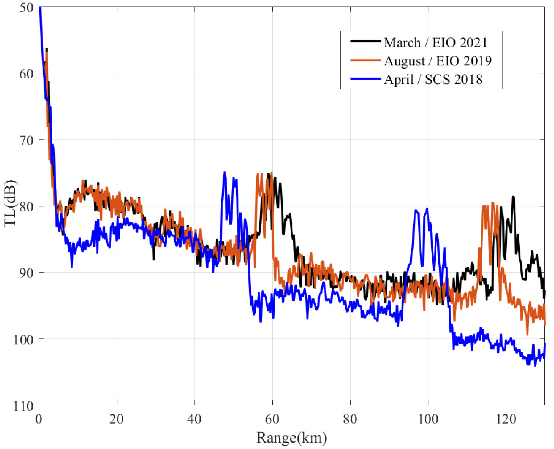
As the table shows, the environmental data and the simulated data of CZ range and width compare very well in both the EOI and SCS. Taking the CZ range in Table 1 for example, the range of the first CZ in the EIO is 7–8 km farther than that in the SCS, and the width of first CZ in the EIO is narrower than that in the SCS.

As explained above, when the water depth is not sufficiently deep, sound speed excess cannot provide sufficient space for sound ray refraction. The sound wave will interact with the bottom to cause rapidly energy decay, and the CZ cannot be formed. In order to analyze the influence of water depth on the CZ, we interchange the water depth of the EIO and the SCS in simulation. The simulation results using the SSP in the EIO and the water depth in the SCS is shown in Figure 14.

Figure 14 shows that the CZ range is also about 58 km. Combined with the simulation result in Figure 9a, we can see that for the same SSP but different water depth, the location of the CZ is basically the same. For the same water depth, the location of the CZ will be significantly different for different SSPs. When the CZs occur, the water depth has little effects on the CZ range. For the same SSP, the greater water depth, the greater depth excess, the greater angle range for sound ray emitted at the source forming a CZ. The CZ width at the same receiving depths becomes wider for greater water depth because of the larger grazing angle.

4. Conclusions

Experiments were carried out in the EIO to obtain new data of acoustic transmission loss to study CZ sound propagation. The sound channel axis in the EIO is deep and there is an extensive constant sound speed layer in the channel. The special environmental characteristics affect sound propagation significantly. Considering the different sound channel in the EIO and the SCS area, the relationship between the structure of SSP and the CZ is analyzed. An expression for the horizontal range that can be used to forecast the first CZ range in deep water area has been deduced, and the expression is demonstrated by the experiment data and model simulation results in this paper.

In summary, we analyze the characteristics of the deep-water CZ using acoustic signals recorded in the experiments conducted in the EIO in 2019 and 2021 at different seasons and in the SCS in 2018. Through the experimental data collected with the different propagation conditions in the EIO and the SCS, we observe that the SSPs in different marine environments have a significant impact on the deep water CZ. The CZ range is mainly affected by the sound channel mixing layer and the isothermal layer, but little affected by the thermocline layer when the depth of the conjugate depth of the ocean bottom is below the surface mixed layer. We study the effects on the CZ characteristics for different environment parameters. The SSP structure strongly affects the CZ range, which can result in 7–8 km offset of the CZ range. The surface mixed layer and the thermocline affect the CZ width but have little effect on the CZ range when conjugate depth of the seabed is below the surface mixed layer. When the propagation conditions change with different seasons in the EIO, the range of the first CZ is almost the same, but the width of the CZs in the summer is narrower about 2 km than in the spring. Because the sound speeds at the source and the bottom are almost the same, the changes in the thermocline affect CZ propagation. The water depth affects the depth excess, which determines the quantity of refracting sound ray clusters, and then affects the CZ width but has little effect on the CZ range. The results in this paper are of great significance to underwater acoustic detection and long-distance acoustic communication in deep water areas of the EIO.

References

1. Liu, B.S.; Lei, J.Y. Principles of Underwater Acoustics; Harbin Engineering University Press: Harbin, China, 1997; pp. 256–262. [Google Scholar]
2. Urick, R.J. Caustics and Convergence Zones in Deep-Water Sound Transmission. J. Acoust. Soc. Am. 1965, 38, 348–358. [Google Scholar] [CrossRef]
3. Henrick, R.F.; Burkom, H.S. The effect of range dependence on acoustic propagation in a convergence zone environment. J. Acoust. Soc. Am. 1983, 73, 173–182. [Google Scholar] [CrossRef]
4. Kevin, D.H.; Richard, L.C.; James, J.M. Detection performance modeling and measurements for convergence zone (CZ) propagation in deep water. J. Acoust. Soc. Am. 2011, 130, 2530. [Google Scholar]
5. Brekhovskikh, L.M.; Lysanov, Y.P. Fundamentals of Ocean Acoustics, 3rd ed.; Springer Press: New York, NY, USA, 2003; pp. 450–460. [Google Scholar]
6. Baggeroer, A.B.; Scheer, E.K.; Heaney, K.; D’Spain, G.; Worcester, P.; Dzieciuch, M. Reliable acoustic path and convergence zone bottom interaction in the Philippine Sea 09 Experiment. J. Acoust. Soc. Am. 2010, 128, 2385. [Google Scholar] [CrossRef]
7. Jensen, F.B.; Kuperman, W.A.; Porter, M.B.; Schmidt, H. Computational Ocean Acoustics, 2nd ed.; Springer: New York, NY, USA, 2011; pp. 337–402. [Google Scholar] [CrossRef] [Green Version]
8. Stephen, D.L.; Gerald, L.D. Investigating sources of variability of the range and structure of the low frequency shallow convergence zone. J. Acoust. Soc. Am. 2011, 130, 2555. [Google Scholar]
9. John, A.C.; Daniel, L.R. Observations of upper ocean sound-speed structures in the North Pacific and their effects on long-range acoustic propagation at low and mid-frequencies. J. Acoust. Soc. Am. 2020, 148, 2040–2060. [Google Scholar]
10. Beilis, A. Convergence zone positions via ray-mode theory. J. Acoust. Soc. Am. 1983, 74, 171–180. [Google Scholar] [CrossRef]
11. Bongiovanni, K.P.; Siegmann, W.L.; Ko, D.S. Convergence zone feature dependence on ocean temperature structure. J. Acoust. Soc. Am. 1996, 100, 3033–3041. [Google Scholar] [CrossRef]
12. Paul, C.E. Underwater Acoustic Modeling and Simulation, 5th ed.; CRC Press: New York, NY, USA, 2018; pp. 103–110. [Google Scholar]
13. Zhang, R.H.; He, Y.; Liu, H. WKBZ normal wave method in horizontal invariant channel. Acta Acust. 1994, 19, 24–34. [Google Scholar]
14. Zhang, X.; Zhang, Y.G.; Dong, N. Effects of thermocline structure variations on acoustic propagation in convergence zone. J. Oceanogr. Taiwan Strait 2011, 30, 114–121. [Google Scholar]
15. Zhuang, Y.F.; Zhang, X.; Liu, Y. Analysis on the influence of sound speed profile structure change in deep sea on convergence zone deflection. Mar. Sci. Bull. 2013, 32, 45–52. [Google Scholar]
16. Cheng, C. Effect of environment dependence of convergence zones in the tropical and subtropical sea areas of western pacific. In Proceedings of the 2016 IEEE/OES China Ocean Acoustics (COA), Harbin, China, 9–11 January 2016. [Google Scholar]
17. Fan, P.Q.; Da, L.L.; Li, Y.Y. Research on characteristic parameter computation method of convergence zones in deep ocean. J. Ocean Tec. 2012, 31, 23–25. [Google Scholar]
18. Lin, S.Y.; Hu, J.H.; Yuan, J.; Zhang, W. Sonar detection performance model and simulation in deep sea convergence zone. In Proceedings of the 2018 IEEE 3rd International Conference on Cloud Computing and Internet of Things (CCIOT), Dalian, China, 20–21 October 2018. [Google Scholar]
19. Li, W.; Li, Z.L.; Zhang, R.H.; Qin, J.; Li, J.; Nan, M. The effects of seamounts on sound propagation in deep water. Chin. Phys. Lett. 2015, 32, 064302. [Google Scholar] [CrossRef]
20. Li, Z.L.; Dong, F.C.; Hu, Z.G.; Wu, S. Vertical correlations of sound field at large depths in deep water. Acta Acust. 2019, 68, 134305. [Google Scholar] [CrossRef]
21. Piao, S.C.; Li, Z.Y.; Wang, X.H.; Zhang, M. Lower turning point convegence zone in deep water with an incomplete channel. Acta. Phys. Sin. 2021, 70, 024301. [Google Scholar] [CrossRef]
22. Liu, D.; Li, Z.L.; Wang, G.X.; Liu, Y.F. Sound Propagation with Undulating Bottom in Shallow Water. J. Mar. Sci. Eng. 2021, 9, 1010. [Google Scholar] [CrossRef]
23. Collins, M.D. A split-step Padé solution for the parabolic equation method. J. Acoust. Soc. Am. 1993, 93, 1736–1742. [Google Scholar] [CrossRef]
24. Wu, S.L.; Li, Z.L.; Qin, J.X. Geoacoustic Inversion for Bottom Parameters in the Deep-Water Area of the South China Sea. Chin. Phys. Lett. 2015, 32, 124301. [Google Scholar] [CrossRef]
25. Porter, M.B.; Bucher, H.P. Gaussian beam tracing for computing ocean acoustic fields. J. Acoust. Soc. Am. 1987, 82, 1349–1359. [Google Scholar] [CrossRef]
Figure 1. The site of the EOI Experiment 2019 and 2021 (Area I) and SCS Experiment 2018 (Area II).
Jmse 10 00424 g001
Figure 2. Experimental configuration.
Jmse 10 00424 g002
Figure 3. Sound speed profiles and bathymetries in the EIO and SCS experiments.
Jmse 10 00424 g003
Figure 4. Bathymetry and SSP along the propagation tracks in the EIO 2019 (a), SCS 2018 (b), and EIO 2021(c) experiments.
Jmse 10 00424 g004aJmse 10 00424 g004b
Figure 5. (a)The signal of source level and (b) the curve of sound source level with frequency 50–2000 Hz (interval 50 Hz).
Jmse 10 00424 g005
Figure 6. Comparison of the experimental and numerical TLs (a) For the propagation track of EIO 2019 at the receiving depth of 255 m; (b) for the propagation track of SCS 2018 at the receiving depth of 255 m; (c) for the propagation track of EIO 2021 at the receiving depth of 285 m.
Jmse 10 00424 g006aJmse 10 00424 g006b
Figure 7. The stratification of the sound speed profile at depth (a) and the sound rays (b) in the EIO.
Jmse 10 00424 g007
Figure 8. Linearized sound speed profile and the sound rays.
Jmse 10 00424 g008
Figure 9. Two-dimensional TLs for the environments of the EIO 2019 (a), EIO 2021 (b), and SCS 2018 (c).
Jmse 10 00424 g009
Figure 10. Comparison of numerical TLs at the depth of 255 m.
Jmse 10 00424 g010
Figure 11. Sound rays for the environments of the EIO (red line) and SCS (black line).
Jmse 10 00424 g011
Figure 12. Maximum emission angle of the ray with different source depth for forming a CZ in the three experiments.
Jmse 10 00424 g012
Figure 13. The detailed changes of sound speed profile in shallow surface of the EIO and SCS.
Jmse 10 00424 g013
Figure 14. Simulated TLs for the SSP in the EIO and water depth in the SCS.
Jmse 10 00424 g014