Underwater Image Restoration via DCP and Yin–Yang Pair Optimization

Abstract

Underwater image restoration is a challenging problem because light is attenuated by absorption and scattering in water, which can degrade the underwater image. To restore the underwater image and improve its contrast and color saturation, a novel algorithm based on the underwater dark channel prior is proposed in this paper. First of all, in order to reconstruct the transmission maps of the underwater image, the transmission maps of the blue and green channels are optimized by the proposed first-order and second-order total variational regularization. Then, an adaptive model is proposed to improve the first-order and second-order total variation. Finally, to solve the problem of the excessive attenuation of the red channel, the transmission map of the red channel is compensated by Yin–Yang pair optimization. The simulation results show that the proposed restored algorithm outperforms other approaches in terms of the visual effects, average gradient, spatial frequency, percentage of saturated pixels, underwater color image quality evaluation and evaluation metric.

1. Introduction

Underwater images play a crucial role in marine biology research, resource detection, underwater target detection and recognition, etc. [1]. However, harsh underwater environments with dissolved organic compounds, concentrations of inorganic compounds, bubbles in the water, water particles, etc., seriously affect the quality of underwater imaging [2]. Underwater images with low contrast, color deviation or distortion have prevented the development of marine-science research. Thus, developing an effective image-processing method to improve underwater image quality is very essential.

To improve the accuracy of underwater target recognition, some scholars have proposed various solutions. Generally, these solutions can be divided into three categories: additional information, image enhancement and physics models. In previous research, additional information such as multiple images or polarization filters were used to improve underwater image quality [3,4,5]. Although these methods are simple and effective, they cannot be used in complex scenes or turbid underwater environments. For the image enhancement algorithms, Lu et al. [6] employed weighted guided trigonometric filtering and artificial light correction for underwater image enhancement, but the time complexity of trilateral filtering is high. Ulutas et al. [7] proposed a methodology that included pixel-center regionalization and global and local histogram equalization with multi-scale fusion to correct color and enhance the image contrast. However, due to the use of the histogram equalization algorithm, this algorithm increased the image noise while improving the image contrast. Ancuti et al. [8] achieved better results by combining the Laplacian contrast, contrast, saliency and exposure features of white-balanced, color-corrected images and the exposure fusion algorithm. However, several results were color shifted because of the exposure process; selecting the exposed images is difficult. In letter [9], a weakly supervised color transformation technique inspired by cycle-consistent adversarial networks (CCANs) was introduced for color correction. However, it has complex network structures with long training times and relies on large amounts of training data. The dark channel prior (DCP) based on the physical model is now widely applied in underwater image restoration [10,11,12]. For example, Galdran used the DCP red channel compensation method to achieve color correction and visibility improvement [13]. Li et al. proposed underwater image restoration based on blue–green channels dehazing and red channel correction [14]. Gao et al. came up with the bright channel prior, which was inspired by the DCP [15]. Although the problems of low contrast and color deviation in underwater images are improved with the above methods, they cannot balance texture enhancement, noise suppression and visual enhancement. To solve these problems, several improved DCP algorithms have been proposed [16,17,18,19]. Combining the DCP with the variation method may be one of the optimal methods because it has the advantages of convenient numerical calculation expressions, good stability, etc. [20,21,22]. Hou et al. used non-local variation, total variation and curvature-total variation to optimize underwater images, respectively [19,23,24]. In the variation method, the regularization parameter plays a key role in local smoothing constraints or texture preservation. However, the regularization parameters are usually set as constants for computational convenience. This will cause a decrease in the restored image quality. Hence, some researchers attempted to adjust the regularization parameters in variation modal adaptively. Liao et al. used generalized cross-validation to select the regularization parameters [25]. Langer et al. proposed an automated parameter selection algorithm which can select scalar or locally varying regularization parameters for total variation models [26]. The discrepancy rule-based method is used for parameter selections [27,28]. Ma et al. established an energy function for regularization parameters [29].

In this paper, a novel algorithm based on the underwater dark channel prior is proposed. The algorithm comprises the following steps in turn: (1) An optimization model combining high-order total variation and first-order total variation is proposed. The first-order variational model is used to preserve the texture in the edge, and the high-order total variation is used to suppress the background noise. (2) A method for selecting the regularization parameters is proposed, which can update the parameters while optimizing the images. (3) The alternating direction method of multipliers (ADMM) is used to improve the calculation speed. (4) The transmission map and the background light of the red channel estimator are compensated by the Yin–Yang pair optimization. The experiments demonstrate that the quality of the restored images can be significantly improved by the proposed algorithm.

2. Background

2.1. Underwater Imaging Model

The propagation of light underwater is a complicated process. According to the Jaffe–McGlamery model [30], the underwater-imaging model can be divided into three components: the direct illumination E_D, the back-scattering E_B and the forward-scattering of light floating E_F [31,32]. The underwater-imaging model E_T can be expressed as:

$$E_T=E_D+E_B+E_F$$

(1)

Due to the scattering and absorption of the particles in the water, only part of the light reaches the camera. Thus, at each image coordinate x, E_D is expressed as:

$$E_D\left(x\right)=J\left(x\right)t\left(x\right)$$

(2)

where J is the ideal image and t is the transmission map. When the optical medium is assumed to be homogeneous, the transmission map t is often estimated by Equation (3):

$$t(x)=\exp \left(-\beta d\left(x\right)\right)$$

(3)

where β is the attenuation coefficient and d is the image depth. Thus, Equation (2) can be transformed as:

$$E_D(x)=J\left(x\right)\exp \left(-\beta d\left(x\right)\right)$$

(4)

The backscattered component results from the interaction between the illumination source and the floating particles dispersed in the water. Therefore, E_B can be expressed as:

$$E_B\left(x\right)=B\left(1-t\left(x\right)\right)=B\left(1-\exp \left(-\beta d\left(x\right)\right)\right)$$

(5)

where B is a color vector of the background light. Schechner and Karpel have shown that backscattering is the main reason for the deterioration of underwater visibility [6]. Thus, forward scattering E_F can be neglected. The simplified underwater-image-information model can be rewritten as:

$$I\left(x\right)=J\left(x\right)t\left(x\right)+B\left(1-t\left(x\right)\right)$$

(6)

where I is the underwater image which is captured by underwater optical imaging equipment. To obtain a better original image, it is essential to estimate B, which can be described as:

$$B=\underset{y\in \mathsf{\Omega }}{\max }\underset{x\in I}{\min }\left\{\underset{c}{\min }{I}^c\left(y\right)\right\}\begin{array}{ccc}& & c\in \left\{R,G,B\right\}\end{array}$$

(7)

where Ω_X is a square local patch centered at x, and c represents the color channel. It is well known that the DCP is widely applied in estimating the transmission map t(x). He et al. found that one of the R, G, B channels for a local area in the non-sky images is almost zero [10]. Based on prior experience, the dark channel is defined as follows:

$$J_{dark}\left(x\right)=\underset{y\in \mathsf{\Omega }}{\min }\left\{\underset{c}{\min }{J}^c\left(y\right)\right\}=0,\begin{array}{ccc}& & c\in \left\{R,G,B\right\}\end{array}$$

(8)

Due to the severe attenuation of the red channel, underwater pictures are in the presence of blue or green wavelengths. Wen proposed the underwater dark channel prior (UDCP) by only considering the blue and green channels [27]. The concept of the UDCP is redefined as:

$$J_{udark}=\underset{y\in \mathsf{\Omega }}{\min }\left\{\underset{c}{\min }{J}^c\left(y\right)\right\}=0\begin{array}{ccc}& & c\in \left\{G,B\right\}\end{array}$$

(9)

Combining with Equations (6) and (9), the result is represented as follows:

$$\underset{y\in \mathsf{\Omega }}{\min }\left\{\underset{c}{\min }\frac{I^c\left(y\right)}{B^c}\right\}=J_{udark}+1-t_{DCP}\left(x\right),\begin{array}{ccc}& & c\in \left\{G,B\right\}\end{array}$$

(10)

The transmission map t_DCP(x) can be written as follows:

$$t_{DCP}\left(x\right)=1-\underset{y\in \Omega }{\min }\left\{\underset{c}{\min }\frac{I^c\left(y\right)}{B^c}\right\}$$

(11)

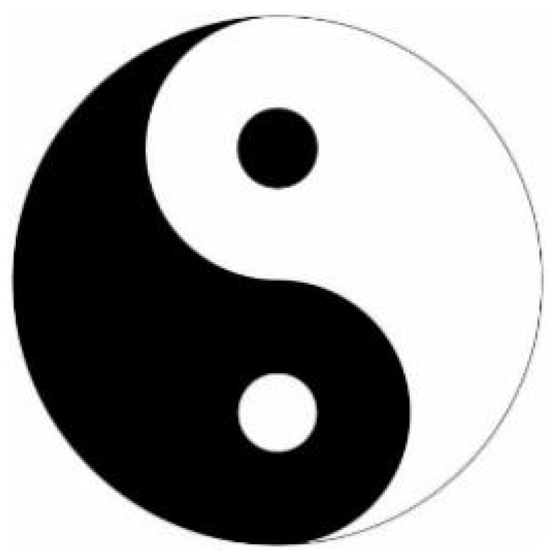
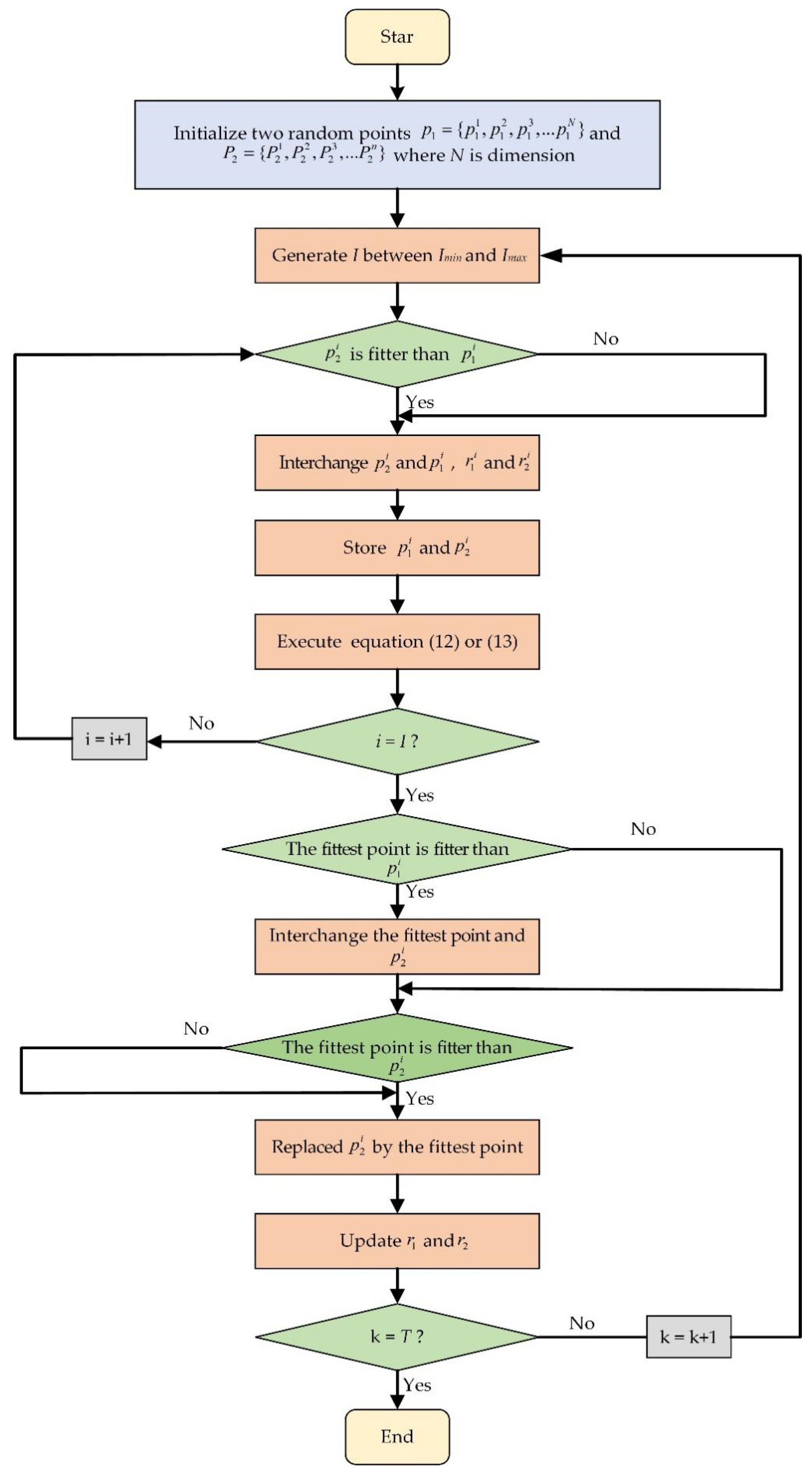
2.2. Yin–Yang Pair Optimization

Yin–Yang pair optimization (YYPO) is a novel metaheuristics optimization [33]. The algorithm uses the traditional Chinese concept of Yin and Yang balance to effectively balance exploration and development. The balance of Yin and Yang in Chinese culture is shown in Figure 1; white and black represent Yang and Yin, respectively, which can be regarded as exploration and exploitation in YYPO. Exploitation plays a vital role in the exploration phase because it may help algorithms jump out of the locally optimal solution. Exploration will make the algorithms converge quickly and reduce the running time in the exploitation phase. This method has a strong exploration and development-balance ability and can effectively estimate the optimal solution. The algorithm has been widely used in the engineering field [34,35,36] but it is still relatively rare in underwater image restoration.

In the initialization phase of YYPO, two random points are generated in the domain of [0, 1]ⁿ and their fitness is evaluated, where n is the dimension of the variable space. The fitter one is named P₁, which is mainly used for development, and the other is named P₂, which is mainly used to explore the variable space. In YYPO, the minimum and the maximum number of archive updates (I_max and I_min), the expansion/contraction factor (α) and the search radius of P₁ and P₂ (r₁ and r₂) are planned. There are two stages in YYPO.

In the splitting stage, although both points experience the splitting stage, only one point along with its search radium (r) undergoes the splitting stage at a time. This is implemented by one of the following two methods and is decided based on an equal probability:

$$S_j^j=S^j+\delta r\begin{array}{cc}& {\mathrm{and} S}_{n+j}^j=\end{array}{S}^j-\delta r,j=1,2,3\dots n$$

(12)

Or:

$$S_{j_2}^{j_1}=\{\begin{array}{c}{S}_{j_2}^{j_1}+{\delta }_1\left(\frac{r}{\sqrt{2}}\right)\begin{array}{ccc}& & {\delta }_2>0.5\end{array}\\ S_{j_2}^{j_1}-{\delta }_1\left(\frac{r}{\sqrt{2}}\right)\begin{array}{ccc}& & {\delta }_2\le 0.5\end{array}\end{array}$$

(13)

In Equation (12), the subscript represents the number of points, and the superscript represents the number of the decision variable being modified, while δ is a random number between 0 and 1. In Equation (13), j₁ is the point number, j₂ represents the decision variable number and δ₁ and δ₂ denote a random number between 0 and 1, respectively. In the archive stage, the stage starts after the required number of archive updates is reached. It should be noted that the archive stage contains 2I points at this stage, and two points (P₁ or P₂) are added during each update before the recovery stage. The search radius will be updated by Equation (14).

$$\{\begin{array}{c}{r}_1=r_1-\frac{r_1}{\alpha }\\ r_2=r_2-\frac{r_2}{\alpha }\end{array}$$

(14)

At the end of the archiving stage, the algorithm determines whether it has reached the maximum number of iterations T. If yes, it will output the result, and if not, it will reset the archiving matrix, and then, the number of archive updates I is randomly generated between I_min and I_max. The flowchart of YYPO is illustrated in Figure 2.

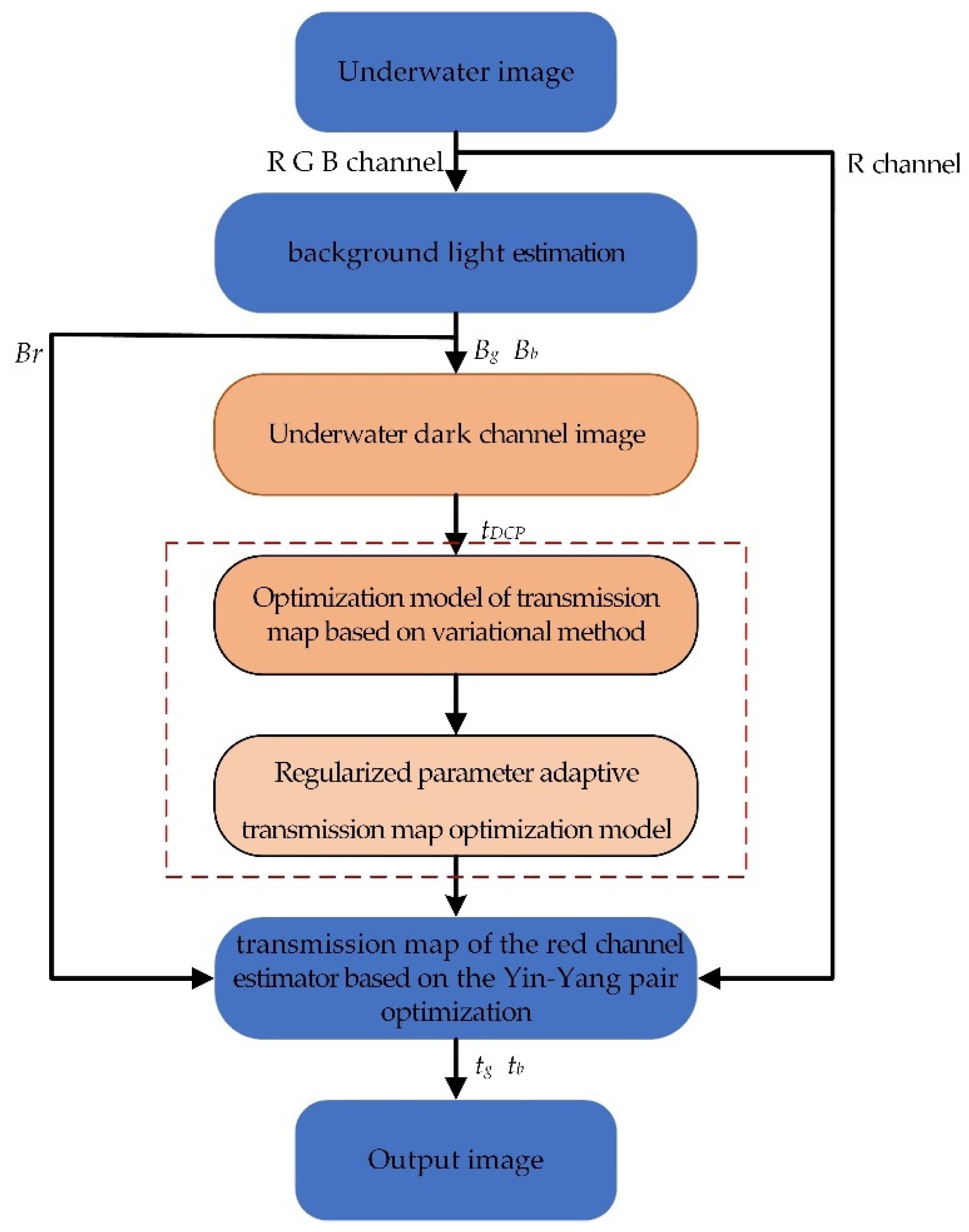
3. Proposed Novel Model

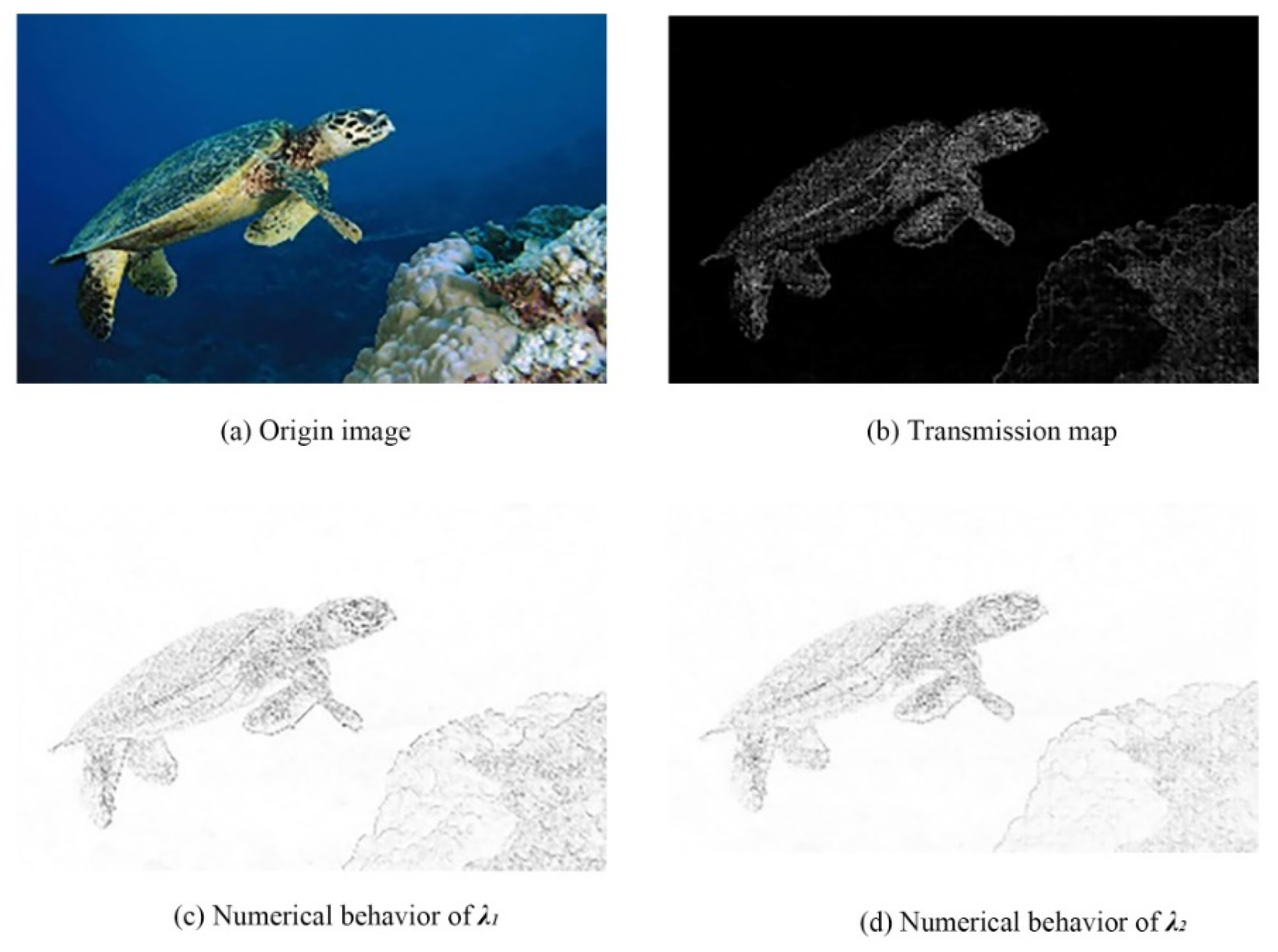
3.1. Novel Transmission Map Optimization Model

In underwater images, first-order variation can preserve sharp features and texture, but staircase artifacts and false edges will appear; the second-order variational smooth ability is strong but it will lose the feeble texture. The following transmission optimization model is proposed as follows:

$$E_1\left(t,J\right)=\Vert {\lambda }_1\circ \epsilon \left(\left|Dt\right|\right)\Vert +\Vert {\lambda }_2\circ D^{2}J\Vert +\frac{1}{2}{\Vert I-Jt-B\left(1-t\right)\Vert }_2^2+\frac{1}{2}{\Vert t-t_{DCP}\Vert }_2^2$$

(15)

where λ₁, λ₂ are the regularization parameters, t_DCP is the transmission map of the underwater DCP estimation, D and D² are the first-order and the second-order difference operators and ԑ( ) is the smoothness metric function, which can be shown as follows:

$$\epsilon \left(\left|\nabla t\right|\right)={\alpha }^2\ln \left(1+\frac{\left|\nabla t\right|}{{\alpha }^2}\right)$$

(16)

where α is a constant and is the first-order variation of t.

In Equation (15), the first term is the first-order variation of the transmittance map, the second term is the second-order variation of the restored image, the third term is the data-fidelity term of the transmissivity map and the fourth term is the data-fidelity term of the restored image. The first-order variation of the transmission map can preserve edges and textures, and through second-order variation, the possible staircase artifacts and noise are smoothed. The problem of Equation (15) is mathematically ill-posed. To improve the computational efficiency of the model, the ADMM algorithm was designed from Equation (15) in this paper, and it introduced three auxiliary variables o, p and q, which are shown in Equation (17):

$$\begin{array}{l}o=\nabla t\\ p=\nabla J\\ q=\Delta J=\nabla p\end{array}$$

(17)

Therefore, Equation (15) can deform into Equation (18):

$$\begin{array}{ll}J=\underset{t,J,o,p,q}{\arg \min }& \{\Vert {\lambda }_1\circ \epsilon \left(\left|o\right|\right)\Vert +\frac{1}{2}{\Vert t-t_{DCP}\Vert }_2^2+\frac{{\theta }_1}{2}{\Vert o-Dt\Vert }_2^2+\hfill \\ & \Vert {\sigma }_1\circ \left(o-Dt\right)\Vert +\Vert {\lambda }_2\circ \left|p\right|\Vert +\hfill \\ & \frac{1}{2}{\Vert I-Jt-\left(1-t\right)B\Vert }_2^2+\frac{{\theta }_2}{2}{\Vert p-DJ\Vert }_2^2+\hfill \\ & \Vert {\sigma }_2\circ \left(p-DJ\right)\Vert +\frac{{\theta }_3}{2}{\Vert q-D^{2}J\Vert }_2^2+\Vert {\sigma }_3\circ \left(q-D^{2}J\right)\Vert \}\hfill \end{array}$$

(18)

where θ₁, θ₂ and θ₃ are the penalty parameters and σ₁, σ₂ and σ₃ are the Lagrangian multipliers. Thus, Equation (18) can be decomposed into five simpler minimization subproblems. Let k be the current number of iterations; the subproblems are shown below:

$$\{\begin{array}{l}{t}^{k+1}=\underset{t}{\arg \min }E\left(t^k,J^k,o^k,p^k,q^k\right)\\ o^{k+1}=\underset{o}{\arg \min }E\left(t^{k+1},J^k,o^k,p^k,q^k\right)\\ J^{k+1}=\underset{J}{\arg \min }E\left(t^{k+1},J^k,o^{k+1},p^k,q^k\right)\\ p^{k+1}=\underset{p}{\arg \min }E\left(t^{k+1},J^{k+1},o^{k+1},p^k,q^k\right)\\ q^{k+1}=\underset{q}{\arg \min }E\left(t^{k+1},J^{k+1},o^{k+1},p^{k+1},q^k\right)\end{array}$$

(19)

Firstly, solve t_k+1 by fixing J_k, o_k, p_k and q_k; the Euler–Lagrange equation for t_k+1 can be expressed as Equation (20):

$$\{\begin{array}{cc}\left(t-t_{DCP}\right)+D{\sigma }_1^k-{\theta }_{1}D\left(Dt-o^k\right)+t{\left(B-J^k\right)}^2+\left(I-B\right)\left(B-J^k\right)=0,\hfill & \hfill \mathrm{in} \Omega \\ \left(-{\sigma }_1^k+{\theta }_1\left(Dt-o^k\right)\right)\cdot n=0,\hfill & \hfill \mathrm{on} \partial \Omega \end{array}$$

(20)

Fix t_k+1, J_k, p_k and q_k to calculate o_k+1. The generalized soft-threshold formulation is given by the equation:

$$o^{k+1}=\max \left[\left|D{t}^{k+1}-\frac{{\sigma }_1^k}{{\theta }_1}\right|-\frac{{\lambda }_1}{{\theta }_1}\cdot \frac{2{\alpha }^2\left|o^k\right|}{{\alpha }^2+{\left(\left|o^k\right|\right)}^2} , 0\right]\cdot \frac{D{t}^{k+1}-\frac{{\sigma }_1^k}{{\theta }_1}}{\left|D{t}^{k+1}-\frac{{\sigma }_1^k}{{\theta }_1}\right|}, 0\frac{0}{\left|0\right|}=0$$

(21)

The J_k+1, p_k+1 and q_k+1 can calculate the generalized soft-threshold formula and the Euler–Lagrangian equation by the above method.

$$\{\begin{array}{cc}J{t}^2-It+t\left(1-t\right)B-{\theta }_{2}D\left(DJ-p^k\right)+D{\sigma }_2^k=0,\hfill & \hfill \mathrm{in} \Omega \\ \left({\theta }_2\left(p^k-DJ\right)+{\sigma }_2^k\right)\cdot n=0\hfill & \hfill \mathrm{on} \Omega \end{array}$$

(22)

$$q^{k+1}=\max \left[\left|D\left(p^k\right)-\frac{{\sigma }_2^k}{{\theta }_2}\right|-\frac{{\lambda }_2}{{\theta }_2},0\right]\cdot \frac{D\left(p^k\right)-\frac{{\sigma }_2^k}{{\theta }_2}}{\left|D\left(p^k\right)-\frac{{\sigma }_2^k}{{\theta }_2}\right|},0\frac{0}{\left|0\right|}=0$$

(23)

$$\{\begin{array}{cc}{\theta }_2\left(p-D{J}^{k+1}\right)+{\sigma }_2^k+D{\sigma }_3^k+{\theta }_{3}D\left(q^{k+1}-Dp\right)=0,\hfill & \hfill \mathrm{in} \Omega \\ \left({\theta }_3\left(q^{k+1}-Dp\right)+{\sigma }_3^k\right)\cdot n=0,\hfill & \hfill \mathrm{on} \Omega \end{array}$$

(24)

Then, the Lagrangian multiplier will be updated as follows:

$$\{\begin{array}{c}\begin{array}{c}{\sigma }_1^{k+1}={\sigma }_1^k+{\theta }_1\left(o^{k+1}-D{t}^{k+1}\right)\\ {\sigma }_2^{k+1}={\sigma }_2^k+{\theta }_2\left(p^{k+1}-D{J}^{k+1}\right)\end{array}\\ {\sigma }_3^{k+1}={\sigma }_3^k+{\theta }_3\left(v^{k+1}-D^2{J}^{k+1}\right)\end{array}$$

(25)

Finally, Equations (22)–(24) can be solved by the Gauss–Seidel iterative method and fast Fourier transform.

3.2. Transmission Map Optimization Model of Regularization Parameters

A parameter selection model is proposed in Equation (26) to adjust the regularization parameters adaptively. This model can optimize the underwater image while selecting the parameters:

$$E_2\left(t,J,{\lambda }_1,{\lambda }_2\right)=E_1\left(t,J,{\lambda }_1,{\lambda }_2\right)+F_1\left({\lambda }_1,{\lambda }_2\right)$$

(26)

where E₁ is from Equation (15) and the function F₁(λ₁, λ₂) is the data-fidelity term for the regularization parameter; therefore, energy function E₂ can be written as:

$$\begin{array}{ll}{E}_2\left(t,J,{\lambda }_1,{\lambda }_2\right)=& {\Vert {\lambda }_1\circ \epsilon \left(\left|Dt\right|\right)\Vert }_F+{\Vert {\lambda }_2\circ D^{2}J\Vert }_F+\\ & \frac{1}{2}{\Vert I-Jt-B\left(1-t\right)\Vert }_E^2+\frac{1}{2}{\Vert t-t_{DCP}\Vert }_E^2\hfill \\ & \frac{a_1}{2}{\Vert {\lambda }_1-b\Vert }_E^2+\frac{a_2}{2}{\Vert {\lambda }_2-b\Vert }_E^2\hfill \end{array}$$

(27)

E₂ can be decomposed to two subproblems. The first subproblem is shown in Equation (15), which was employed to estimate t and J, and the second subproblem, which solves λ₁ and λ₂, can be expressed as:

$$\left({\lambda }_1,{\lambda }_2\right)=\underset{{\lambda }_1,{\lambda }_2}{\arg \min }{\Vert {\lambda }_1\circ \epsilon \left(\left|Dt\right|\right)\Vert }_1+{\Vert {\lambda }_2\circ D^{2}J\Vert }_1+\frac{a_1}{2}{\Vert {\lambda }_1-b\Vert }_2^2+\frac{a_2}{2}{\Vert {\lambda }_2-b\Vert }_2^2$$

(28)

where a₁, a₂ and b are positive numbers. To calculate λ₁ and λ₂, the ADMM is used again. The subproblem of the energy function E₂ is:

$$\{\begin{array}{c}{\lambda }_1=\underset{\lambda 1}{\arg \min }\left({\Vert {\lambda }_1\circ \epsilon \left(\left|Dt\right|\right)\Vert }_F+\frac{a_1}{2}{\Vert {\lambda }_1-b\Vert }_E^2\right)\\ {\lambda }_2=\underset{\lambda 2}{\arg \min }\left({\Vert {\lambda }_2\circ D^{2}J\Vert }_F+\frac{a_2}{2}{\Vert {\lambda }_2-b\Vert }_E^2\right)\end{array}$$

(29)

By calculating Equation (29), λ₁ and λ₂ can be obtained:

$$\{\begin{array}{c}{\lambda }_1=\frac{a_{1}b-\epsilon \left(Dt\right)}{a_1}\\ {\lambda }_2=\frac{a_{2}b-D^{2}J}{a_2}\end{array}$$

(30)

It is vital to research the numerical behavior of λ₁ and λ₂ corresponding to the regions of t and J at different scales, such as texture or background. Figure 3a is an underwater image. Figure 3b is the second-order differential of (a). Figure 3c,d are the numerical behaviors of λ₁ and λ₂, respectively.

In Figure 3, we show the numerical behavior of λ₁ and λ₂. In the background regions, the λ₁ and λ₂ are large. In the texture regions, the λ₁ and λ₂ are small. In the underwater image, the sharp edge of the water scattering forms a large number of slope regions. In the ramp region, the gradient of t is inversely proportional to λ₁ and λ₂. In the variational model, the values of the regularization parameter control the relative weights of the fidelity and regularization terms. More precisely, when the values of the regularization parameter are small, the regularization is also small. When the values of the regularization parameter are large, over-regularization may occur. In conclusion, in the background region, the regularization parameter is large, which can smooth the staircase artifacts and false edges; in the texture region, the small regularization parameter can protect the texture; in the ramp region, the feature of the regularization parameter can enhance texture and reduce the width of the ramp.

3.3. Red Compensation Based on Yin–Yang Pair Optimization

Under water, the attenuation of red light is much greater than that of green light, so the background light and transmission map of the red channel estimated by the DCP cannot be used directly. In this section, an estimator of the transmission and the background light of the red channel based on YYPO is proposed.

Due to the high correlation between the red, green and blue channels, compensating for the red channel alone may make the restored image redder. Therefore, this section proposes a red-channel-transmission-map estimator based on YYPO. Zhao et al. [37,38] discovered the relationship between the transmission map of the red channel and the blue–green channel, as shown by Equations (31) and (32):

$$t_b\left(x\right)=t_r{\left(x\right)}^{\frac{{\beta }_b}{{\beta }_r}}=t_r{\left(x\right)}^{\frac{B_r\left(m{\lambda }_b+i\right)}{B_b\left(m{\lambda }_r+i\right)}}$$

(31)

$$t_g\left(x\right)=t_r{\left(x\right)}^{\frac{{\beta }_g}{{\beta }_r}}=t_r{\left(x\right)}^{\frac{B_r\left(m{\lambda }_g+i\right)}{B_g\left(m{\lambda }_r+i\right)}}$$

(32)

where B_r, B_g and B_b are the ground lights of the red, green and blue channel, respectively. λ_r, λ_g and λ_b are the wavelengths of red, green and blue light, m = −0.00113, i = 1.62517. According to Equations (31) and (32), the objective function of YYPO can be defined as:

$$f_{red}\left(t_r\right)={\Vert t_r-t_b{}^{\frac{B_b\left(m{\lambda }_r+i\right)}{B_r\left(m{\lambda }_b+i\right)}}\Vert }_2^2+{\Vert t_r-t_g{}^{\frac{B_g\left(m{\lambda }_r+i\right)}{B_r\left(m{\lambda }_g+i\right)}}\Vert }_2^2$$

(33)

$$t_r=1-\underset{y\in \Omega }{\min }\left(\frac{I_r}{B_r}\right)$$

(34)

where I_r is the red channel of the original underwater image. Search tr continuously through YYPO to calculate the value of Equation (33). When the minimum value of Equation (33) is obtained, the optimal Br can be estimated by Equation (34). The t_r is estimated by t_g and t_b, which are optimized by Sections 3.1 and 3.2. A framework of the proposed method is presented in Figure 4. Inside the red dotted line is the acceleration part using the ADMM algorithm.

4. Experiments and Discussions

4.1. Evaluation of Objectives and Approaches

In this section, the effectiveness of the proposed models is assessed. To ensure the fairness and the objective of all algorithms, they were implemented on a Windows 10 PC with Intel(R) Core (TM) i7-8700U CPU@3.20GHz, 16.00GB, running Python3.7.

In the experiment, the effectiveness of the proposed algorithm was evaluated from two aspects:

(1) To examine the superiority of the proposed algorithm with restoration algorithms;

(2) To assess the superiority of the proposed algorithm with synthesized underwater images.

In Experiment (1), several different types of algorithms were used to validate the proposed algorithm, including the algorithm for wavelength compensation and image de-hazing (WCID) [39], blue–green channels de-hazing and red channel correction (ARUIR) [14], guided image filtering (GIF) [18] and underwater light attenuation prior (ULAP) [40]. Experiment (1) includes two parts: quantitative analysis and subjective analysis. Quantitative analysis is performed by using the average gradient (AG), spatial frequency (SF), percentage of saturated pixels (PS), underwater color image quality evaluation (UCIQE) [41] and the blind referenceless image spatial quality evaluator (BRISQUE) [42]. The IE, AG and SF reflect the number of edges and textures in the image. The number of edges and textures is proportional to the AG and SF. However, the underwater image restoration algorithm may amplify noise, and the noise will increase the AG and SF. Therefore, when using the AG and SF to evaluate the restored image, it is necessary to combine the restored image itself for evaluation. The PS judges the restored image by calculating the ratio between the number of saturated pixels and the total pixels. When the PS is small, the effect of the restoring image is better. The UCIQE takes chroma, saturation and contrast as the measurement components and linearly combines the measurement components to estimate the quality of the image. BRISQUE is an unreferenced image estimation method. When the score of BRISQUE is lower, the image quality is better. In experiment (2), to evaluate the restoration imageability of the proposed algorithm, we used the method proposed by Gao et al. [15] for underwater image synthesis and adopted the peak signal-to-noise ratio (PSNR) and structural similarity (SSIM) to assess the quality of the picture. The PSNR represents the restoration accuracy between pixels, and the SSIM represents the similarity between image textures.

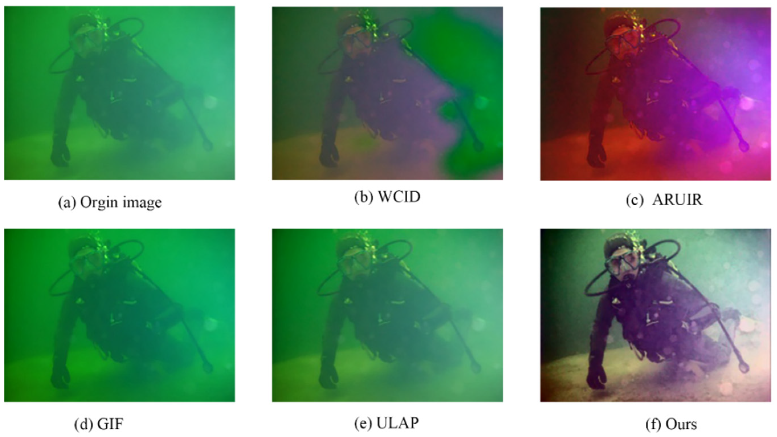
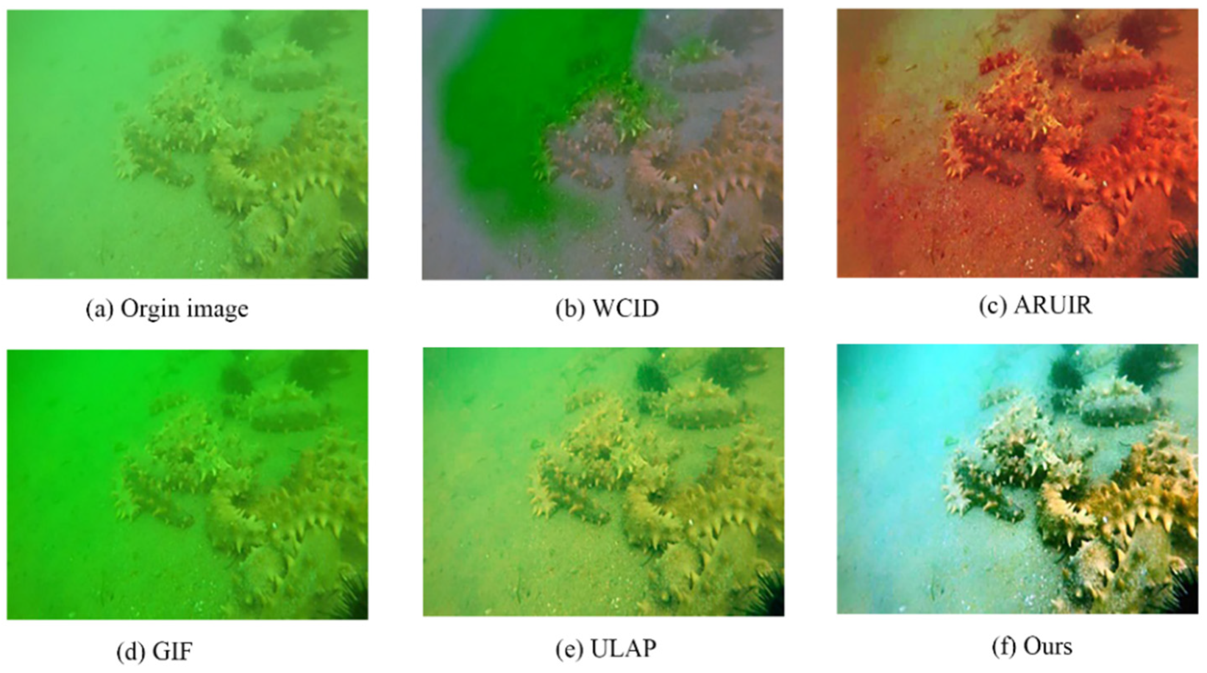
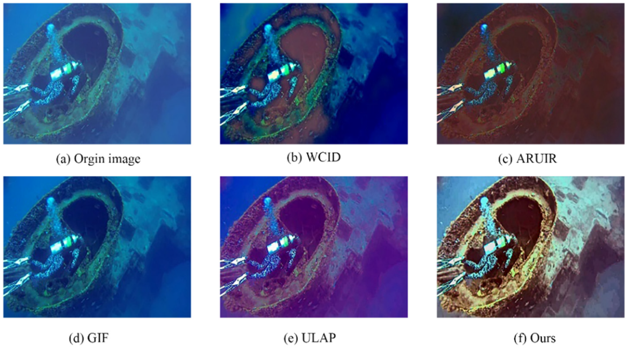
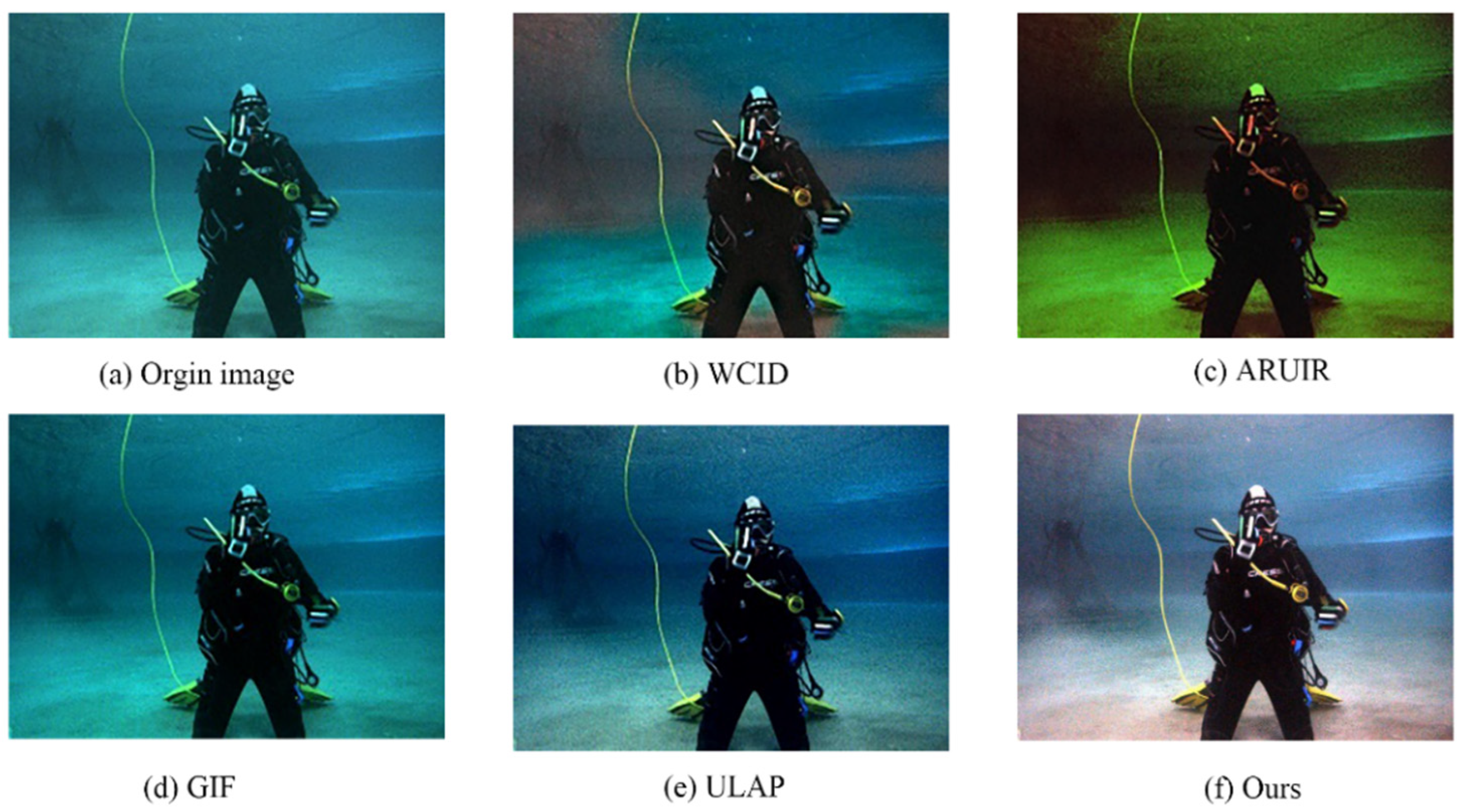
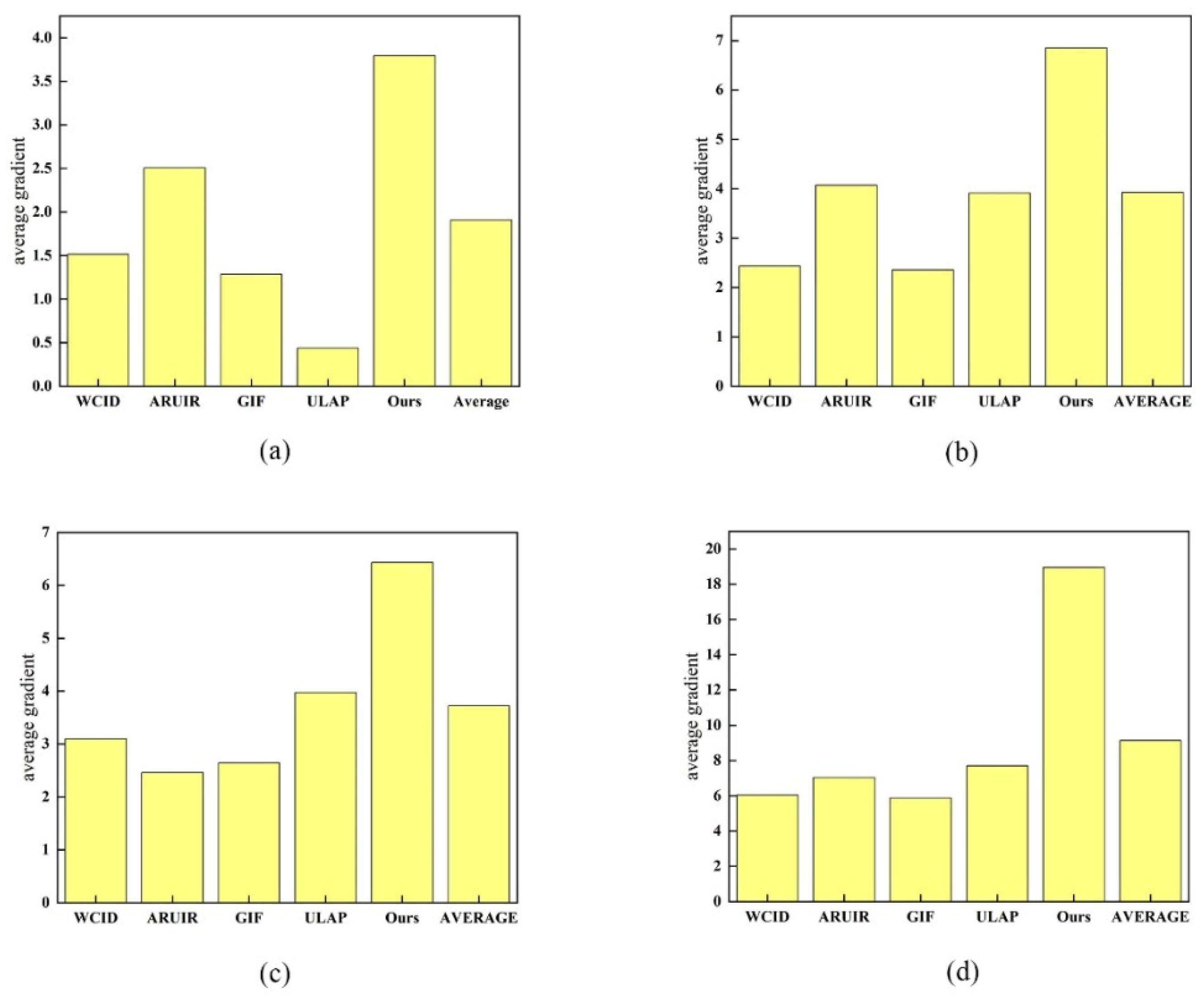
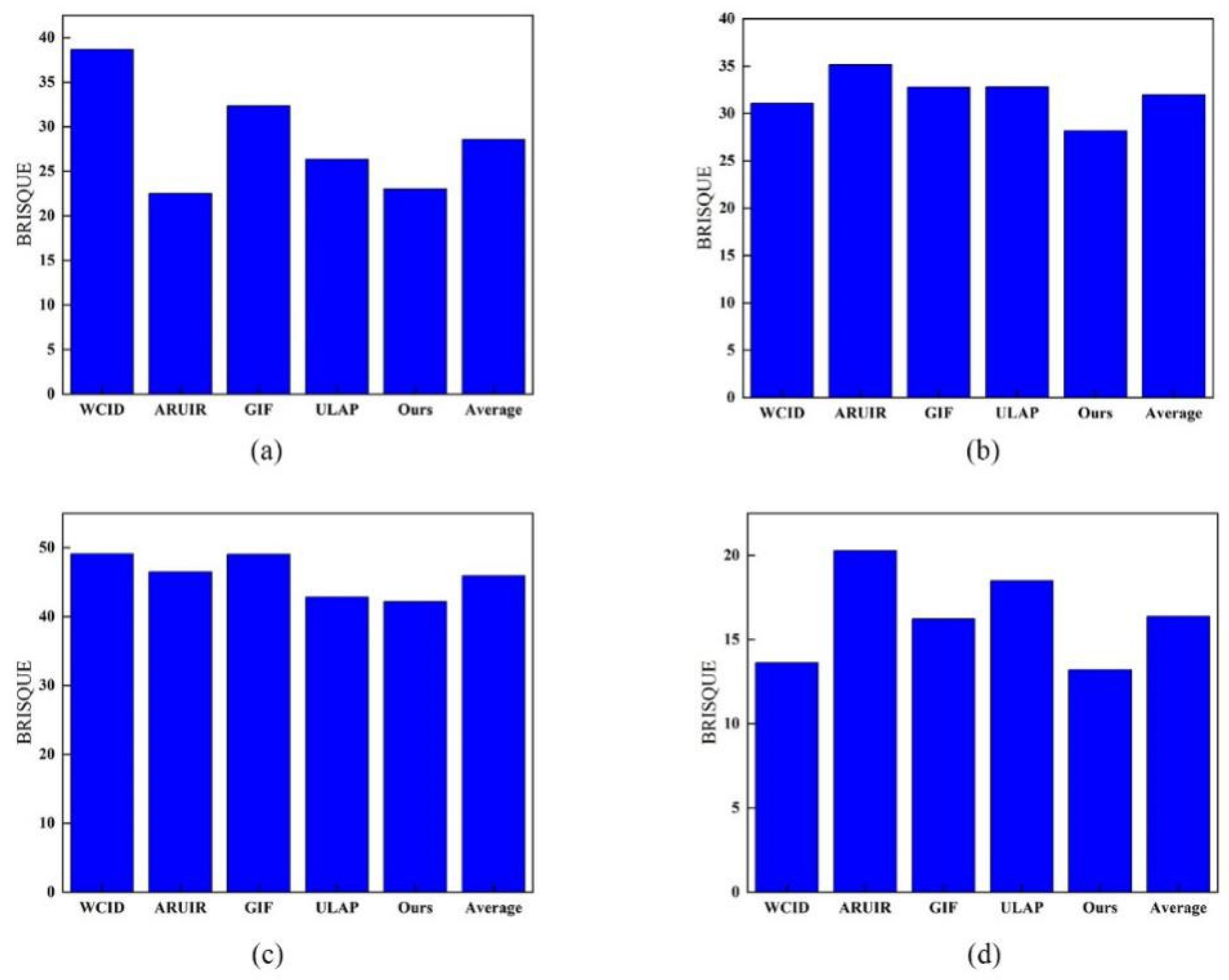
4.2. No Reference Image Restoration Effect Evaluation

In this section, the superiority of the proposed algorithm is verified by real images. It is difficult to evaluate the quality of underwater images because there is no reference standard since there is no ground truth or uniform measure standard available. So, we chose pictures from four different-colored scenes (Figure 5a, Figure 6a, Figure 7a, Figure 8a) that gradually changed from green to blue and compared the algorithm in Section 4.1 with our algorithm. In the transmission-map-optimization model based on the first-order and high-order variational models, the maximum number of iterations is 30, a₁ = a₂ = 1, b = 0.05. The selection of these parameters is the same as that proposed by Punnathanam [33]. Figure 5b–f are the restored images via WCID, ARUIR, GIF, ULAP and ours.

Table 1. Quantitative analysis of Figure 5.

	SF	PS	UCIQE
WCID	0.065	0.075	0.416
ARUIR	0.052	0.006	0.533
GIF	0.058	0.265	0.423
ULAP	0.049	0.062	0.046
Ours	0.073	0.018	0.572

,

Table 2. Quantitative analysis of Figure 6.

	SF	PS	UCIQE
WCID	0.063	0.15	0.405
ARUIR	0.057	0.005	0.489
GIF	0.051	0.074	0.361
ULAP	0.054	0.005	0.438
Ours	0.068	0.064	0.595

,

Table 3. Quantitative analysis of Figure 7.

	SF	PS	UCIQE
WCID	0.06	0.284	0.627
ARUIR	0.047	0.003	0.533
GIF	0.041	0.198	0.553
ULAP	0.053	0.048	0.583
Ours	0.067	0.017	0.626

and

Table 4. Quantitative analysis of Figure 8.

	SF	PS	UCIQE
WCID	0.061	0.142	0.583
ARUIR	0.06	0.049	0.535
GIF	0.077	0.237	0.552
ULAP	0.125	0.234	0.562
Ours	0.173	0.084	0.65

are the assessment results of the restored images including the SF, PS and UCIQE. Additionally, we calculated the AG and BRISQUE for these four kinds of images, as shown in Figure 9 and Figure 10.

Figure 5a is the original underwater image. Figure 5b,c have a serious problem of color deviation. Figure 5e has low contrast, and the restored image is green. The contrast is high in Figure 5f, and its recovery result is more realistic than the others. However, the corners of Figure 5f are black. From Table 1, Figure 5f, Figure 9a and Figure 10a are the best in the AG and UCIQE. The SF of the restored images is almost identical. Because the corners of Figure 5f are black, the PS and the BRISQUE are not the best.

From Figure 6b, the contrast is low, and there are color deviations in the restored image. The phenomenon of red channel overcompensation appears in the restored image. The recovery effect of Figure 6c–e are poor because the algorithm does not have red correction. Figure 6f is still green because the assumption that the red channel is the weakest is invalid. However, compared with the other algorithms, the contrast and visual effect of the restored image is better. The same conclusion can be drawn from Table 2, Figure 9b and Figure 10b; the AG, SF, UCIQE and BRISQUE are the best in Figure 6f.

Different from Figure 5a, Figure 6 and Figure 7a is the level of blue. In Figure 7b–d, they all have the problem of low contrast, and a lot of the texture and edges are missing. The restored image Figure 7f is the best because the contrast and visual effect are excellent. From Table 3, Figure 9c and Figure 10c show that the restored image Figure 7f, obtained by the proposed algorithm, has an advantage in everything except the PS.

Figure 8a is also blue. From the perspective of the restoration effect, Figure 8f has a higher restoration degree, but from the PS, the quality of Figure 8f is low because there is a lot of visible noise. Table 4, Figure 9d and Figure 10d also support this conclusion; the UCIQE is the best image and BRISQUE is the worst one. Because of the noise, the AG is also the largest.

It can be seen from Figure 5f, Figure 6, Figure 7 and Figure 8f that the proposed algorithm can choose different regularization parameters for the target and background regions. The edge and texture details of the target are effectively preserved in the target area. In the background area, the noise is effectively suppressed while improving the image quality, so the regularization parameter selection process is of great significance.

4.3. Full Reference Image Restoration Effect Evaluation

In this section, since there is no ground-truth database available for underwater images, to evaluate the performance of the proposed approach more objectively, we quantitatively analyzed the resilience of the algorithm by using synthetic images. Figure 11 is the original image which was obtained in sunny weather.

According to [15] and the actual underwater situation, four different background lights are set: B₁ = [0.35, 0.51, 0.28], B₂ = [0.17, 0.43, 0.33], B₃ = [0.29, 0.21, 0.47] and B₄ = [0.12, 0.26, 0.38]. These four different background lights make the histogram of the synthesis images different. The synthesis images and background light can be shown as Figure 12.

Figure 12a–d are the synthesis images in which the background lights are B1, B2, B3 and B4, respectively. Each group of images in Figure 12 from left to right is the color of the background light and the synthesis images. Moreover, the PSNR and SSIM are shown in

Table 5. Full reference evaluation.

	PSNR	SSIM
WCID	19.34	0.814
ARUIR	21.91	0.836
GIF	21.16	0.827
ULAP	20.47	0.833
Ours	22.74	0.849

.

From Table 5, the best PSNR is the restored images of the proposed algorithm, which shows that the algorithm can effectively restore the intensity of the image. As can be seen from Table 5, the proposed restoration algorithm achieves the best performance among the compared methods in terms of the SSIM.

5. Conclusions

A novel underwater image restoration algorithm is proposed in this paper based on the DCP and Yin–Yang pair optimization. The algorithm is composed of four important parts: combining the first-order variational and the high-order variational transmission-map-optimization model, the adaptive parameter selection method, the solution of the transmission-map-optimization model via the ADMM, the red channel transmittance map and the background light estimator. The algorithm is executed on a set of representative real and synthesized underwater images which demonstrate that it can enhance the detailed texture features of the image while suppressing background noise. Moreover, a large number of qualitative and quantitative experimental comparison results further ensure that the recovered underwater images have better quality than others’ works. In addition, completely discarding the red channel when calculating the transmittance map of green and red channels may cause it to be overcompensated. We need to find a way to solve this problem considering the red channel in the future.

References

1. Ancuti, C.O.; Ancuti, C.; De Vleeschouwer, C.; Bekaert, P. Color Balance and Fusion for Underwater Image Enhancement. IEEE Trans. Image Process. 2018, 27, 379–393. [Google Scholar] [CrossRef] [PubMed] [Green Version]
2. Drews, P., Jr.; do Nascimento, E.; Moraes, F.; Botelho, S.; Campos, M. Transmission Estimation in Underwater Single Images. In Proceedings of the 2013 IEEE International Conference on Computer Vision Workshops, Sydney, Australia, 2–8 December 2013. [Google Scholar]
3. Amer, K.O.; Elbouz, M.; Alfalou, A.; Brosseau, C.; Hajjami, J. Enhancing underwater optical imaging by using a low-pass polarization filter. Opt. Express 2019, 27, 621–643. [Google Scholar] [CrossRef] [PubMed]
4. Boffety, M.; Galland, F.; Allais, A.G. Influence of Polarization Filtering on Image Registration Precision in Underwater Conditions. Opt. Lett. 2012, 37, 3273–3275. [Google Scholar] [CrossRef] [PubMed]
5. Narasimhan, S.G.; Nayar, S.K. Contrast restoration of weather degraded images. IEEE Trans. Pattern Anal. Mach. Intell. 2003, 25, 713–724. [Google Scholar] [CrossRef] [Green Version]
6. Lu, H.; Li, Y.; Xu, X.; Li, J.; Liu, Z.; Li, X.; Yang, J.; Serikawa, S. Underwater image enhancement method using weighted guided trigonometric filtering and artificial light correction. J. Vis. Commun. Image Represent. 2016, 38, 504–516. [Google Scholar] [CrossRef]
7. Ulutas, G.; Ustubioglu, B. Underwater image enhancement using contrast limited adaptive histogram equalization and layered difference representation. Multimed. Tools Appl. 2021, 80, 15067–15091. [Google Scholar] [CrossRef]
8. Ancuti, C.; Ancuti, C.O.; Haber, T. Enhancing underwater images and videos by fusion. In Proceedings of the 2012 IEEE Conference on Computer Vision & Pattern Recognition, Providence, RI, USA, 16–21 June 2012. [Google Scholar]
9. Li, C.; Guo, J.; Guo, C. Emerging from water: Underwater image color correction based on weakly supervised color transfer. IEEE Signal Proc. Let. 2018, 25, 323–327. [Google Scholar] [CrossRef] [Green Version]
10. He, K.; Sun, J.; Tang, X. Single Image Haze Removal Using Dark Channel Prior. IEEE Trans. Pattern Anal. Mach. Intell. 2011, 33, 2341–2353. [Google Scholar]
11. Peng, Y.T.; Cosman, P.C. Underwater Image Restoration Based on Image Blurriness and Light Absorption. IEEE Trans. Image Process. 2017, 26, 1579–1594. [Google Scholar] [CrossRef]
12. Yu, H.; Li, X.; Lou, Q.; Lei, C.; Liu, Z. Underwater image enhancement based on DCP and depth transmission map. Multimed. Tools Appl. 2020, 79, 27–28. [Google Scholar] [CrossRef]
13. Galdran, A.; Pardo, D.; Picon, A.; Alvarez-Gila, A. Automatic Red-Channel underwater image restoration. J. Vis. Commun. Image Represent. 2015, 26, 132–145. [Google Scholar] [CrossRef] [Green Version]
14. Li, C.; Quo, J.; Pang, Y.; Chen, S.; Jian, W. Single underwater image restoration by blue-green channels dehazing and red channel correction. In Proceedings of the 2016 IEEE International Conference on Acoustics, Speech and Signal Processing (ICASSP), Shanghai, China, 20–25 March 2016. [Google Scholar]
15. Gao, Y.; Li, H.; Wen, S. Restoration and Enhancement of Underwater Images Based on Bright Channel Prior. Math. Probl. Eng. 2016, 2016, 3141478. [Google Scholar] [CrossRef]
16. Yang, H.Y.; Chen, P.Y.; Huang, C.C.; Zhuang, Y.Z.; Shiau, Y.H. Low Complexity Underwater Image Enhancement Based on Dark Channel Prior. In Proceedings of the 2011 Second International Conference on Innovations in Bio-Inspired Computing and Applications, Shenzhen, China, 16–18 December 2011. [Google Scholar]
17. Peng, Y.T.; Cao, K.; Cosman, P.C. Generalization of the Dark Channel Prior for Single Image Restoration. IEEE Trans. Image Process. 2018, 27, 2856–2868. [Google Scholar] [CrossRef]
18. He, K.; Sun, J.; Tang, X. Guided image filtering. IEEE Trans. Pattern Anal. Mach. Intell. 2010, 35, 1397–1409. [Google Scholar] [CrossRef]
19. Hou, G.; Pan, Z.; Wang, G.; Yang, H.; Duan, J. An efficient nonlocal variational method with application to underwater image restoration. Neurocomputing 2019, 369, 106–121. [Google Scholar] [CrossRef]
20. Song, M.; Qu, H.; Zhang, G.; Tao, S.; Jin, G. A Variational Model for Sea Image Enhancement. Remote Sens. 2018, 10, 1313. [Google Scholar] [CrossRef] [Green Version]
21. Tan, L.; Liu, W.; Pan, Z. Color image restoration and inpainting via multi-channel total curvature. Appl. Math. Model. 2018, 61, 280–299. [Google Scholar] [CrossRef]
22. Liu, J.; Ma, R.; Zeng, X.; Liu, W.; Wang, M.; Chen, H. An efficient non-convex total variation approach for image deblurring and denoising. Appl. Math. Comput. 2021, 397, 259–268. [Google Scholar] [CrossRef]
23. Hou, G.; Li, J.; Wang, G.; Pan, Z.; Zhao, X. Applications, Underwater image dehazing and denoising via curvature variation regularization. Multimed. Tools Appl. 2020, 79, 20199–20219. [Google Scholar] [CrossRef]
24. Hou, G.; Li, J.; Wang, G.; Yang, H.; Huang, B.; Pan, Z. A novel dark channel prior guided variational framework for underwater image restoration. J. Vis. Commun. Image Represent. 2020, 66, 102732. [Google Scholar] [CrossRef]
25. Liao, H.Y.; Fang, L.; Michael, K.N. Selection of regularization parameter in total variation image restoration. J. Opt. Soc. Am. 2009, 26, 2311–2320. [Google Scholar] [CrossRef] [PubMed]
26. Langer, A. Automated Parameter Selection for Total Variation Minimization in Image Restoration. J. Math. Imaging Vis. 2016, 57, 239–268. [Google Scholar] [CrossRef] [Green Version]
27. Wen, Y.W.; Chan, R.H. Parameter selection for total-variation-based image restoration using discrepancy principle. IEEE Trans. Image Process. 2012, 21, 1770–1781. [Google Scholar] [CrossRef] [Green Version]
28. Chen, A.Z.; Huo, X.M.; Wen, Y.W. Adaptive regularization for color image restoration using discrepancy principle. In Proceedings of the 2013 IEEE International Conference on Signal Processing, Communications and Computing (ICSPCC), Kunming, China, 5–8 August 2013. [Google Scholar]
29. Ma, T.H.; Huang, T.Z.; Zhao, X.L. New Regularization Models for Image Denoising with a Spatially Dependent Regularization Parameter. Abstr. Appl. Anal. 2013, 2013, 729151. [Google Scholar] [CrossRef]
30. Wen, H.; Tian, Y.; Huang, T.; Guo, W. Single underwater image enhancement with a new optical model. In Proceedings of the 2013 IEEE International Symposium on Circuits and Systems (ISCAS), Beijing, China, 19–23 May 2013. [Google Scholar]
31. Barros, W.; Nascimento, E.R.; Barbosa, W.V.; Campos, M.F.M. Single-shot underwater image restoration: A visual quality-aware method based on light propagation model. J. Vis. Commun. Image Represent. 2018, 55, 363–373. [Google Scholar] [CrossRef]
32. Yang, M.; Sowmya, A.; Wei, Z.; Zheng, B. Offshore Underwater Image Restoration Using Reflection Decomposition Based Transmission Map Estimation. IEEE J. Ocean. Eng. 2020, 45, 521–533. [Google Scholar] [CrossRef]
33. Punnathanam, V.; Kotecha, P. Yin-Yang-pair Optimization: A novel lightweight optimization algorithm. Eng. Appl. Artif. Intell. 2016, 54, 62–79. [Google Scholar] [CrossRef]
34. Punnathanam, V.; Kotecha, P. Multi-objective optimization of Stirling engine systems using Front-based Yin-Yang-Pair Optimization. Energy Convers. Manag. 2017, 133, 332–348. [Google Scholar] [CrossRef]
35. Yang, B.; Yu, T.; Shu, H.; Zhu, D.; Zeng, F.; Sang, Y.; Jiang, L. Perturbation observer based fractional-order PID control of photovoltaics inverters for solar energy harvesting via Yin-Yang-Pair optimization. Energy Convers. Manag. 2018, 171, 170–187. [Google Scholar] [CrossRef]
36. Song, D.; Liu, J.; Yang, J.; Su, M.; Wang, Y.; Yang, X.; Huang, L.; Joo, Y.H. Optimal design of wind turbines on high-altitude sites based on improved Yin-Yang pair optimization. Energy 2020, 193, 497–510. [Google Scholar] [CrossRef]
37. Zhao, X.; Jin, T.; Qu, S. Deriving inherent optical properties from background color and underwater image enhancement. Ocean Eng. 2015, 94, 163–172. [Google Scholar] [CrossRef]
38. Jiao, Q.; Liu, M.; Li, P.; Dong, L.; Hui, M.; Kong, L.; Zhao, Y. Underwater Image Restoration via Non-Convex Non-Smooth Variation and Thermal Exchange Optimization. J. Mar. Sci. Eng. 2021, 9, 570. [Google Scholar] [CrossRef]
39. Chiang, J.Y.; Chen, Y.C. Underwater image enhancement by wavelength compensation and dehazing. IEEE Trans. Image Process. 2012, 21, 1756–1769. [Google Scholar] [CrossRef] [PubMed]
40. Song, W.; Wang, Y.; Huang, D.; Tjondronegoro, D. A Rapid Scene Depth Estimation Model Based on Underwater Light Attenuation Prior for Underwater Image Restoration. In Proceedings of the Advances in Multimedia Information Processing—PMC 2018, Hefei, China, 21–22 September 2018. [Google Scholar]
41. Yang, M.; Sowmya, A. An Underwater Color Image Quality Evaluation Metric. IEEE Trans. Image Process. 2015, 24, 62–71. [Google Scholar] [CrossRef] [PubMed]
42. Mittal, A.; Moorthy, A.K.; Bovik, A.C. No-reference image quality assessment in the spatial domain. IEEE Trans. Image Process. 2012, 21, 4695–4708. [Google Scholar] [CrossRef]
Figure 1. Yin and Yang.
Jmse 10 00360 g001
Figure 2. The flowchart of YYPO.
Jmse 10 00360 g002
Figure 3. Numerical behavior of λ1 and λ2.
Jmse 10 00360 g003
Figure 4. Framework of the proposed approach.
Jmse 10 00360 g004
Figure 5. Underwater image enhancement result. (a) The origin image. (b) The result of WCID; (c) the result of ARUIR; (d) the result of GIF; (e) the result of ULAP; (f) the result of ours.
Jmse 10 00360 g005
Figure 6. Underwater image enhancement result. (a) The origin image. (b) The result of WCID; (c) the result of ARUIR; (d) the result of GIF; (e) the result of ULAP; (f) the result of ours.
Jmse 10 00360 g006
Figure 7. Underwater image enhancement result. (a) The origin image. (b) The result of WCID; (c) the result of ARUIR; (d) the result of GIF; (e) the result of ULAP; (f) the result of ours.
Jmse 10 00360 g007
Figure 8. Underwater image enhancement result. (a) The origin image. (b) The result of WCID; (c) the result of ARUIR; (d) the result of GIF; (e) the result of ULAP; (f) the result of ours.
Jmse 10 00360 g008
Figure 9. (a) Figure 5a uses the AG values of different algorithms, (b) Figure 6a uses the AG values of different algorithms, (c) Figure 7a uses the AG values of different algorithms and (d) Figure 8a uses the AG values of different algorithms.
Jmse 10 00360 g009
Figure 10. (a) Figure 5a uses the BRISQUE values of different algorithms, (b) Figure 6a uses the BRISQUE values of different algorithms, (c) Figure 7a uses the BRISQUE values of different algorithms and (d) Figure 8a uses the BRISQUE values of different algorithms.
Jmse 10 00360 g010
Figure 11. Original image.
Jmse 10 00360 g011
Figure 12. (a) Synthesis image by B1, (b) synthesis image byB2, (c) synthesis image byB3 and (d) synthesis image by B4.
Jmse 10 00360 g012