Course Control of a Manta Robot Based on Amplitude and Phase Differences

Abstract

Due to external interference, such as waves, the success of underwater missions depends on the turning performance of the vehicle. Manta rays use two broad pectoral fins for propulsion, which provide better anti-interference ability and turning performance. Inspired by biological yaw modes, we use the phase difference between the pectoral fins to realize fast course adjustment and the amplitude difference to realize precise adjustment. We design a bionic robot with pectoral fins and use phase oscillators to realize rhythmic motion. An expected phase difference transition equation is introduced to realize a fast and smooth transition of the output, and the parameters are adjusted online. We combine the phase difference and amplitude difference yaw modes to realize closed-loop course control. Through course interference and adjustment experiments, it is verified that the combined mode is more effective than a single mode. Finally, a rectangular trajectory swimming experiment demonstrates continuous mobility of the robot under the combined mode.

1. Introduction

In recent years, with the continuous increase in marine engineering projects such as submarine cables, pipeline detection, and oil and gas exploration, the demand for autonomous underwater vehicles (AUVs) has increased [1]. In view of the shortcomings of traditional propulsion methods [2], bionic AUVs adopt new propulsion methods, which have more advantages, such as high efficiency, high mobility and low noise [3,4]. Fish can be divided into two categories according to their propulsion mode: body and caudal fin (BCF) mode and median or paired fin (MPF) mode [5]. BCF fish have better propulsion and acceleration, whereas MPF fish have higher efficiency and mobility at low speed. Many BCF fish also use pectoral fins to realize high mobility [6,7]. According to the wave number of the pectoral fins, an MPF fish can be divided into paired oscillation pectoral fins (OPFs, less than half a wave) and paired undulation pectoral fins (UPFs, more than one wave) [8]. Manta rays and cownose rays are typical OPF batoids, and their locomotion characteristics are very similar [9,10].

Turning performance is an important aspect of an aquatic animal’s locomotor skills, including mobility (turning ability in a confined space) and agility (turning angular velocity). It plays an important role in capturing objects, fleeing predators, avoiding obstacles in complex environments and resisting environmental interference [11,12,13,14,15]. Because there are many underwater disturbances, the completion of an underwater task depends more on mobility than speed [16,17]. Turning performance has always been the focus of most mobility research, especially yaw turning [18]. Because of its two broad pectoral fins, manta rays show better stability under interference [15]. In addition, manta rays have high turning performance, with a turning radius of 0.38 times their body length and a yaw angle velocity of 67.32°/s [19]. In recent years, manta rays have attracted increasing attention from researchers [20,21,22,23,24].

On the one hand, researchers have carried out exploratory research and adopted new propulsion methods, such as phototactic guidance [25], dielectric elastomers [26] and electrofluidic actuators [27]. However, the propulsion capacity of these methods is limited, resulting in limited mobility. They mainly focus on function realization and can accomplish only slow yaw. On the other hand, researchers have developed a variety of bionic robots using conventional propulsion methods, which have good turning performance. A manta robot driven by a shape memory alloy (SMA) has been established [28]. By controlling the swing amplitude of the pectoral fin, a certain turning radius can be realized. Cownose Ray-I was established [29], taking the cownose ray as the bionic object with three fin rays on each side. Depending on the amplitude difference and phase difference of the pectoral fin, yaw angle velocities of 22.5°/s and 45°/s can be realized. A spatial parallel mechanism (SPM) was designed to actively control the deformation of the bionic flapping wing near the fin root, and yaw angle velocities of nearly 50°/s and 60°/s were realized by controlling the amplitude and phase difference of the pectoral fins [30]. However, the above research only realizes an open-loop yaw control of the robot, only quantifies the yaw angle velocity of the robot, and does not realize stable closed-loop course control. The Robo ray robot was established to actively control the fins using flexibility [31]. Depending on the phase difference between the pectoral fins, a yaw angle velocity of 60°/s was realized. In addition, a fuzzy closed-loop strategy was adopted to realize accurate course control. The yaw angle velocity under closed-loop control is 25°/s. The above research has achieved better yaw mobility of a robot, but most of them only achieve faster yaw angle velocity in an open-loop case and only use a single course control mode. They have not studied the precise course control ability of a robot and course adjustment ability under external interference.

Because a sine-based control method has the problem of discontinuous output, artificial central pattern generators (CPGs) composed of nonlinear oscillators have become the mainstream motion control method of robots. At present, the main CPG models include Matsuoka oscillators [32,33], Hopf oscillators [22,34] and phase oscillators [35,36]. Control methods based on CPGs have been successfully applied to several fish-like robots, and switching between different behaviors has been realized. A salamander robot (Salamander I) driven by 10 DC motors was established [37]. By adjusting the two input signals to the CPG model, the speed, direction and gait type of the robot can be adjusted, smooth switching from a crawling gait to a swimming gait can be completed, and a turning action can also be completed. Based on the Salamander I robot, a Salamander II robot was established [38]. Using a single CPG circuit, it realized five behaviors: swimming, struggling, forward underwater walking, forward and backward ground walking, and integrated ontology feedback to optimize swimming speed. To solve the problem of coordinated control of a robot with multiple degrees of freedom, an improved phase oscillator model was established [31], which has the characteristics of controllable amplitude, phase lag, smooth frequency transition and asymmetric oscillation, so that the Robo ray robot has the ability to swim forward, swim backward, yaw and pitch. In addition, a CPG-fuzzy-based control algorithm was developed into vivid and stable three-dimensional motion, and open-loop speed control strategies and closed-loop depth and yaw control were established. The above research realizes online switching between different modes of the robot but does not pay too much attention to the unsmooth output caused by the change in CPG parameters. A snake robot adopts the phase oscillator model as the rhythm output control method [39]. They consider the jump in the expected phase difference and introduce an activation function. For simplicity, a linear two-stage function is selected as the activation function to realize a linear change in the expected phase difference with time. The activation function can reduce the unsmooth output problem caused by the change in expected phase difference, but the causes are not studied. After the introduction of the activation function, the output is still not smooth.

In view of the above problems, this paper mainly studies the reasons for the unsmooth output caused by the change in the expected phase difference, draws lessons from the amplitude transition equation of the phase oscillator, introduces an expected phase difference transition equation, and realizes a smooth transition in the expected phase difference. On this basis, new peaks in the transition process caused by the change in the expected phase difference are avoided, and a smooth transition of the output is realized. In addition, based on the observation and analysis of the biological yaw mode, the advantages and disadvantages of the two yaw modes based on asymmetric amplitude and asymmetric phase difference are compared. The combination of the two yaw modes makes up for the shortcomings of an easy overshoot of the phase difference mode and slow adjustment speed of the amplitude mode to realize the high maneuverability of yaw, no overshoot, rapidity and stability. Through experiments, the advantages of the combined control strategy over a single yaw mode are verified. The combined control strategy has the ability to resist external interference and realize rapid and accurate adjustment of course, and the fastest yaw angle velocity is 62°/s.

2. Materials and Methods

2.1. Yaw Mode Analysis

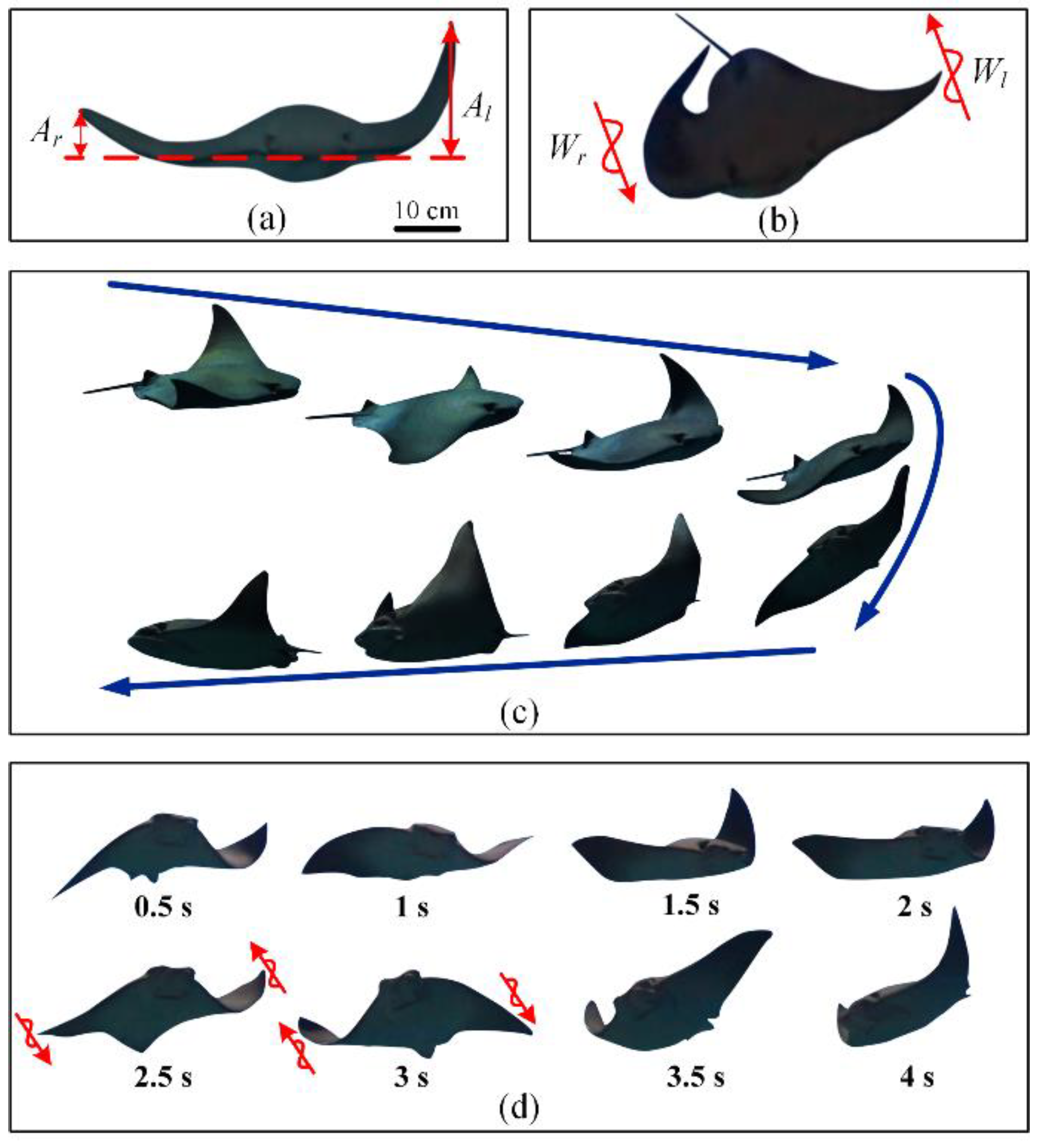
Through the observation and analysis of images and videos collected in the Beijing Aquarium, two main ways to realize the yaw mode of cownose rays were found: different flapping amplitudes and different wave transmission directions of both pectoral fins. In this paper, different flapping amplitudes of both pectoral fins are called asymmetric amplitudes, and different wave transmission directions are called asymmetric phase differences.

Based on the yaw mode of asymmetric amplitude, the flapping amplitude of the pectoral fin on one side is greater than that on the other side (Figure 1a), and the side with the larger flapping amplitude produces a greater propulsive force and lift, resulting in different propulsive forces of the pectoral fins, forming a turning torque and realizing a yaw mode (Figure 1c). When a cownose ray yaws in this way, it is generally accompanied by body tilt and spiral descent. In this way, the ray often mixes the gliding mode and uses a combination of gliding and flapping to adjust course [10,19]. Therefore, the yaw mode based on asymmetric amplitude is suitable for small-amplitude adjustment of course, with a slow yaw angle rate and large yaw radius.

Based on the yaw mode of the asymmetric phase difference, the wave transmission directions of the pectoral fin are different (Figure 1b). The thrust of one pectoral fin is backward, and the thrust of the other is forward to form a large turning torque and realize a faster yaw adjustment (Figure 1d). In this way, a cownose ray can realize high-maneuvering in situ turning, which is generally used to avoid obstacles in front in case of an emergency. Therefore, the yaw mode based on asymmetric phase difference is suitable for large course adjustment with a fast yaw angle rate and small yaw radius.

2.2. Bionic Design of the Structure

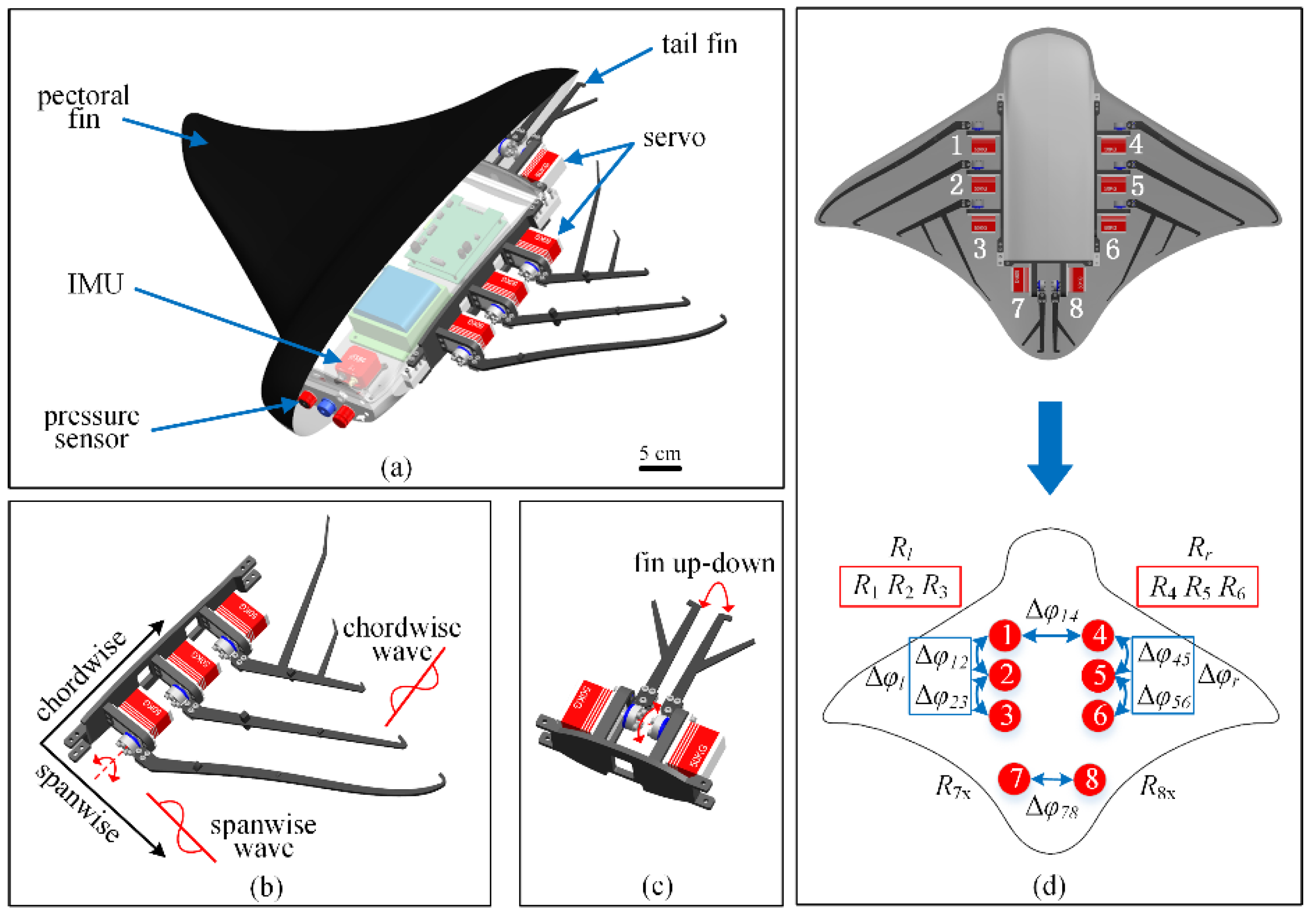
To realize the bionic design of a cownose ray, the bionic robot is mainly composed of a main body structure, pectoral fin structure and tail fin structure (Figure 2a). Because the pectoral fin structure of the robot has an important impact on the performance, the pectoral fin (flapping wing) is designed as three fins on each side, and each fin is driven by a servo. The fins are designed with different lengths and shapes. According to the biological anatomy of a manta ray’s pectoral fin structure, the pectoral fin structure has a variable flexible distribution [40,41] and active and passive deformation during active propulsion. The fins are made of flexible carbon fiber materials, and the thicknesses of the three fins are different to realize the bionic design of the pectoral ray (Figure 2b).

The tail fin of the robot is composed of two servos, which is a bionic design of the tail fin of a cownose ray. The robot has no buoyancy change device and changes the pitch angle by deflecting the tail fin to realize depth control, which is consistent with the actual behavior of a cownose ray (Figure 2c).

The characteristic parameters of the manta robot are shown in

Table 1. Comparison of existing robotic manta.

Item	Robotic Manta [28]	Robotic Manta [29]	Robotic Manta [30]	Robotic Manta [31]	Proposed One
Length (m)	0.243	0.3	0.456	0.58	0.8
Width (m)	0.220	0.5	0.83	0.92	0.6
Weight (Kg)	0.354	1	4.8	6.3	7
Turing method	Amplitude difference	Amplitude/ph-ase difference	Amplitude/ph-ase difference	Phase difference	Amplitude and phase differences
Maximum yaw angle rate (°/s)	-	22.5°/s 45°/s	50°/s 60°/s	25°/s	62°/s
Closed-loop control	No	No	No	Yes	Yes

. The overall dimensions of the robot are 800 mm × 600 mm × 150 mm, and the total mass is 7 kg. The robot is powered by a lithium battery, with an operating time of more than 4 h. It has a flapping frequency of 0.2~0.8 Hz, an amplitude of more than 50°, a swimming speed of −0.5~1 kn (−0.25~0.5 m/s), and a maximum yaw angle rate of 62°/s.

2.3. Phase Oscillator Model

According to the research object and the characteristics of the robot, this paper adopts an improved phase oscillator model, which is mainly composed of a phase equation, amplitude equation, bias equation, expected phase difference equation and output equation.

$${\dot{\varphi }}_i=2\pi v_i+{\displaystyle \sum _j{w}_{ij}}\sin ({\varphi }_j-{\varphi }_i-\Delta {\phi }_{ij})$$

(1)

$${\ddot{r}}_i=a_i\left[\frac{a_i}{4}(R_i-r_i)-{\dot{r}}_i\right]$$

(2)

$${\ddot{x}}_i=b_i\left[\frac{b_i}{4}(X_i-x_i)-{\dot{x}}_i\right]$$

(3)

$$\Delta {\ddot{\phi }}_{ij}=c_i\left[\frac{c_i}{4}(\Delta {\varphi }_{ij}-\Delta {\phi }_{ij})-\Delta {\dot{\phi }}_{ij}\right]$$

(4)

$${\theta }_i=x_i+r_i\sin ({\varphi }_i)$$

(5)

where ${\varphi }_i$, $r_i$, $x_i$, $\mathsf{\Delta }{\phi }_{ij}$ are the phase, amplitude and bias amplitude of oscillator $i$ and the expected phase difference between oscillators $i$ and $j$, respectively. ${\theta }_i$ is the output of oscillator $i$, which is combinedly determined by ${\varphi }_i$, $r_i$, $x_i$. If the bias amplitude is not 0, the output is a sinusoidal signal with bias.

The coupling term of other oscillators to oscillator $i$ can be expressed as:

$$O{C}_i={\displaystyle \sum _j{w}_{ij}}\sin ({\varphi }_j-{\varphi }_i-\Delta {\phi }_{ij})$$

(6)

Equation (1) determines the change in the phase of each oscillator with time, which is key for an oscillator to show a limit cycle behavior. When the oscillator reaches a stable state, the stable phase relationship between different oscillators is ensured. The parameter ${\nu }_i$ is the frequency and is positive. The parameter $\mathsf{\Delta }{\phi }_{ij}$ determines the phase relationship when the two oscillators reach a stable state. The parameter $w_{ij}$ determines the transition time for the oscillator to reach a new stable vibration state, which is positive. The larger the value is, the shorter the transition time and the less smooth the transition. Equation (6) is the coupling term of other oscillators to oscillator $i$. In the transition process, the greater its value ($O{C}_i$) is, the greater the change rate of the phase derivative in Equation (1), the faster the output transition and the worse the smoothness.

Equation (2) is a second-order linear ordinary differential equation with critical damping. The expected amplitude is taken as a stable fixed point, and the coefficient ($a_i$) is positive, which determines the rapidity and smoothness of the amplitude transition. The larger the value ($a_i$) is, the shorter the transition time is, and the worse the smoothness is. Equations (3) and (4) have the same characteristics as (2), and the parameters ($b_i$, $c_i$) are positive numbers, which determine the transition characteristics of transition to and transition from, respectively. The greater the value, the shorter the transition time and the worse the smoothness.

2.4. Construction of the Topology Network Structure

The CPG oscillators adjacent to one side of the pectoral fin of the manta robot are more closely connected, and the CPG oscillators on both sides of the pectoral fin are less connected. We adopt the simplest CPG topology. According to the structural characteristics of the manta robot designed in this paper, oscillators 1 and 4 play a leading role. We adopt the simplest CPG topology and take oscillators 1 and 4 as the reference datum (Figure 2d).

To facilitate a unified description, the expected amplitude of the left pectoral fin is expressed as $R_l$, the expected phase difference is expressed as $\mathsf{\Delta }{\phi }_l$ and output is expressed as ${\theta }_l$. The desired amplitude of the right pectoral fin is expressed as $R_r$, the desired phase difference is expressed as $\mathsf{\Delta }{\phi }_r$, and the output is expressed as ${\theta }_r$. The sign of the expected phase difference does not represent the size but only the wave transmission direction along the chordwise direction, where a negative sign represents forward transmission, and a positive sign represents backward transmission.

3. Results

3.1. Phase Transition Characteristic Analysis

To facilitate the analysis, the phase transition characteristics between the two oscillators are first studied. Taking oscillators 1 and 2 as the analysis objects, the coupling term in the phase equation of oscillator 1 is:

$$O{C}_1=w_{12}\sin ({\varphi }_2-{\varphi }_1-\Delta {\phi }_{12})$$

(7)

where the real-time phase difference is:

$${\varphi }_{12}={\varphi }_2-{\varphi }_1$$

(8)

The difference between the real-time phase difference and the real-time expected phase difference is:

$$\delta {\phi }_{12}={\varphi }_{12}-\Delta {\phi }_{12}$$

(9)

$$O{C}_1=w_{12}\sin (\delta {\phi }_{12})$$

(10)

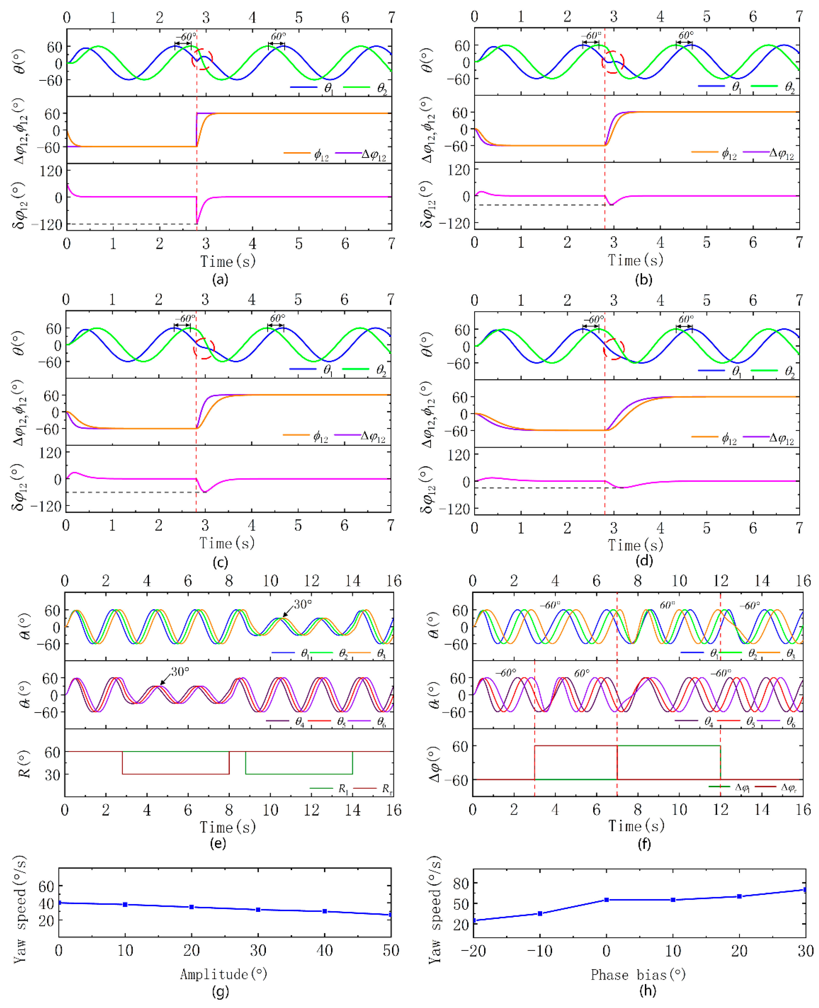
The expected phase difference ($\mathsf{\Delta }{\phi }_{12}$) between the two oscillators changes from −60° to 60°, the coupling weight ($w_{12}$) is 6, the transition coefficient ($c$) is 30 and the frequency ($\upsilon$) is 0.5. First, we analyzed the transition equation without the expected phase difference. Because $\mathsf{\Delta }{\phi }_{12}$ is abrupt, the maximum value of $\mathsf{\delta }{\phi }_{12}$ appears at the beginning of the transition, and a jump in $O{C}_1$ occurs. The change rate of the phase derivative is large, and the output increases first and then decreases, resulting in wave peaks and poor smoothness (Figure 3a). Then, the expected phase difference transition equation is added, and $\mathsf{\Delta }{\phi }_{12}$ is a smooth transition. In the process of the change, the two oscillators also transition to a new stable vibration state, and ${\varphi }_{12}$ is also a smooth transition. The change in $\mathsf{\delta }{\phi }_{12}$ is smoother, and the output is smoother than before the improvement, but the output is still increasing first and then decreasing, resulting in wave peaks (Figure 3b). We try to reduce the coupling coefficient ($w_{12}$) to 3. $O{C}_1$ is determined by $w_{12}$ and sin $\left(\mathsf{\delta }{\phi }_{12}\right)$; the minimum value of $\mathsf{\delta }{\phi }_{12}$ decreases, but $w_{12}$ also decreases. The size of $w_{12}$ has a greater impact on the output, so the output is smoother, avoiding the phenomenon that the output increases first and then decreases (Figure 3c).

We try to analyze how to avoid the phenomenon of the output increasing first and then decreasing. The phase derivative is determined by the frequency and coupling term. The frequency is positive. When the sign of the phase derivative changes, the monotonicity changes. The maximum and minimum values of the coupling term are:

$$\begin{array}{l}O{C}_{1\_\max }=w_{12}\\ O{C}_{1\_\min }=-w_{12}\end{array}$$

(11)

Equation (1) that the maximum and minimum values of the phase derivative correspond to:

$$\begin{array}{l}{\dot{\varphi }}_{1\_\max }=2\pi v+w_{12}\\ {\dot{\varphi }}_{1\_\min }=2\pi v-w_{12}\end{array}$$

(12)

Since the frequency and coupling coefficient are positive, the maximum value of the phase derivative is greater than 0. When the minimum value is less than 0, the phase derivative changes from positive to negative. If the output is in the decreasing range, the output changes from monotonically decreasing to increasing, resulting in a wave crest. At this time, the corresponding conditions are as follows:

$$w_{12}>2\pi v$$

(13)

If the frequency and coupling coefficient meet this condition, the output curve will produce a crest when the expected phase difference changes greatly. If this condition is not satisfied, no matter how much the expected phase difference changes, there will be no crest in the output curve. Since the frequency $\upsilon$ = 0.5, there will be no wave crest when $w_{12}<2\pi \upsilon =3.14$ (Figure 3c) and when $w_{12}=6$, the output will increase, resulting in a wave crest (Figure 3b).

We further reduce the transition coefficient to 10 and reduce the rapidity of the desired phase difference transition, and the output is smoother, but the subsequent impact is a reduction in the rapidity of the output transition (Figure 3d).

3.2. Yaw Mode Simulation

From the yaw mode analysis, it can be seen that the yaw modes of a cownose ray are based on the asymmetric amplitude and asymmetric phase difference of the pectoral fins. A simulation of these two yaw modes is carried out to ensure the rapidity and smoothness of the output in the transition process.

3.2.1. Yaw Mode Based on Asymmetric Amplitude

At the initial stage, the amplitude of the pectoral fins is 60°; when t = 2.8 s, $R_r$ decreases from 60° to 30°. The expected amplitude of the left pectoral fin is greater than that of the right pectoral fin, the thrust generated by the left side is greater than that of the right, and the robot turns right. When t = 8 s, $R_r$ increases from 30° to 60°, and then$R_l$ decreases from 60° to 30°. The thrust generated by the right pectoral fin is greater than that of the left pectoral fin, and the robot turns left (Figure 3e).

3.2.2. Yaw Mode Based on Asymmetric Phase Difference

At the initial stage, when the expected phase difference between the pectoral fin on both sides is −60°, when t = 3 s, $\mathsf{\Delta }{\phi }_r$ changes from −60° to 60°, and $\mathsf{\Delta }{\phi }_l$ remains unchanged. The thrust of the left pectoral fin is forward, and the thrust of the right pectoral fin is backward, realizing a high-maneuvering right turn of the robot. When t = 7 s, $\mathsf{\Delta }{\phi }_r$ changes from 60° to −60° and $\mathsf{\Delta }{\phi }_l$ changes from −60° to 60°, the thrust of the left pectoral fin is backward and the thrust of the right side is forward, which creates a high-maneuvering left turn. When t = 12 s, $\mathsf{\Delta }{\phi }_l$ changes from 60° to −60° and $\mathsf{\Delta }{\phi }_r$ remains unchanged at −60°, the thrust on both sides of the robot is backward, and it is switched from a high-maneuvering mode to a straight swimming mode (Figure 3f).

The simulation results of the two yaw modes show that the control strategy can accomplish a fast smooth transition of the output when the parameters change.

3.3. Yaw Mode Open-Loop Experiments

Based on the observation and analysis of organisms, the two modes have their own advantages and disadvantages. To formulate the strategy for a robot to realize stable course control, open-loop experiments of the two yaw modes are carried out to explore the difference in yaw angle rate.

In the experiment analyzing the yaw mode based on the asymmetric amplitude, the expected phase difference of both pectoral fins is −30°, the frequency is 0.4 Hz, the expected amplitude of one pectoral fin is 60°, and the other side varies from 0° to 50° in increments of 10°, and the corresponding course angular rates are 40°/s, 38°/s, 35°/s, 32°/s, 30°/s, and 25°/s (Figure 3g).

In the experiment analyzing the yaw mode based on the asymmetric phase difference, the amplitude of both pectoral fins is 60°, the frequency is 0.4 Hz, the expected phase difference of one pectoral fin is −30°, and that of the other side varies from −20°to 30° in increments of 10°, and the corresponding course angular rates are 25°/s, 35°/s, 55°/s, 55°/s, 60°/s, and 70°/s (Figure 3h).

The experimental data analysis shows that the yaw angle rate based on the asymmetric phase difference is faster, but the yaw angle rate changes suddenly. When the expected phase difference of one pectoral fin is −30° and the expected phase difference of the other pectoral fin is 0°, the maximum yaw angle rate is close to the maximum. In the yaw mode based on the asymmetric amplitude, the yaw angle rate is slightly slower but changes continuously with the increase in the amplitude difference, and the transition is gentler.

3.4. Closed-Loop Control of Depth and Course

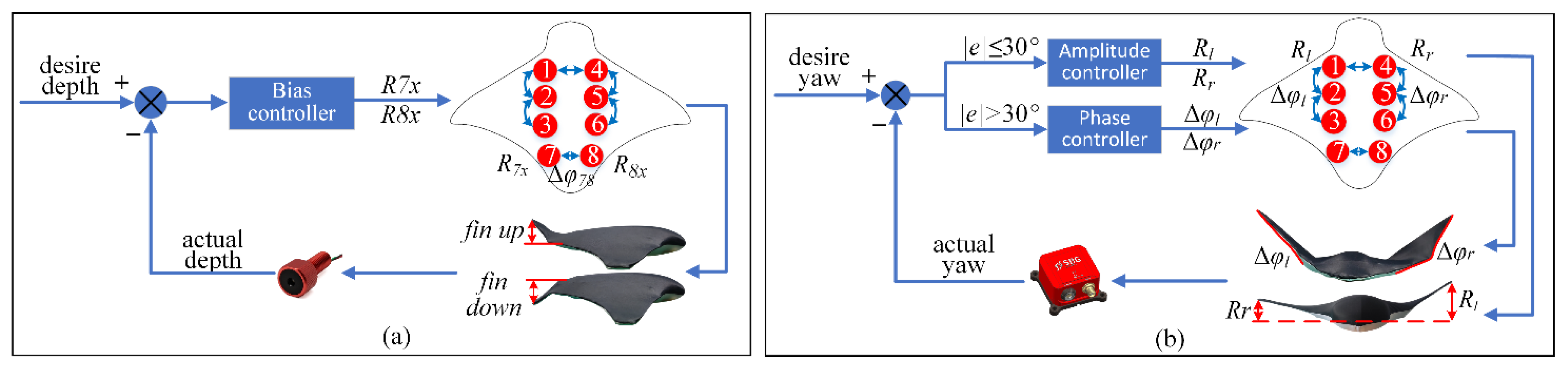
Ensuring that the robot swims underwater is the premise of realizing good turning performance. The pitch angle of the robot is adjusted by using the tail fin deflection to achieve the effect of maintaining the robot within a fixed-depth range (Figure 4a).

To realize the smooth transition of output, this paper introduces a phase transition equation. It takes a certain time for the expected value transition to be completed. The robot needs to change the expected phase difference in advance of reaching the specified course and reserve time to complete the transition of output. At the same time, combined with the characteristics of the two yaw modes, the asymmetric phase difference is used to quickly adjust the course using large deviations, and the asymmetric amplitude is used to accurately and continuously adjust the course using small deviations. In addition, the asymmetric amplitude can change the expected phase difference in advance, ensure the smooth transition of output, and realize rapid and accurate adjustment. If the difference between the current azimuth and the expected azimuth is greater than 30°, the asymmetric phase difference yaw mode is used to accomplish a rapid adjustment. If the difference between the current azimuth and the expected azimuth is less than 30°, the asymmetric amplitude yaw mode is used to accomplish an accurate adjustment of the robot (Figure 4b).

3.5. Course Anti-Interference Experiments

Due to underwater interference such as waves, we try to test the ability to resist external interference. In this case, to verify whether our combined control strategy has more advantages, robot experiments were carried out in a pool (length, width and depth: 10 m, 4.5 m, 1 m).

In the normal forward swimming state, we try to move the robot’s head clockwise in front of the swimming direction using a PVC pipe to make it deviate from the original course by approximately 90°. Due to the uncertainty of human interference, it is difficult to ensure that the interference intensity is completely consistent each time, but the interference is at the same intensity level. We performed interference experiments relying only on the phase difference or amplitude difference and relying on the combined mode of the phase and amplitude difference. The robot starts to have a set yaw and always swims according to the set value, and the actual yaw is the real-time yaw when the robot swims.

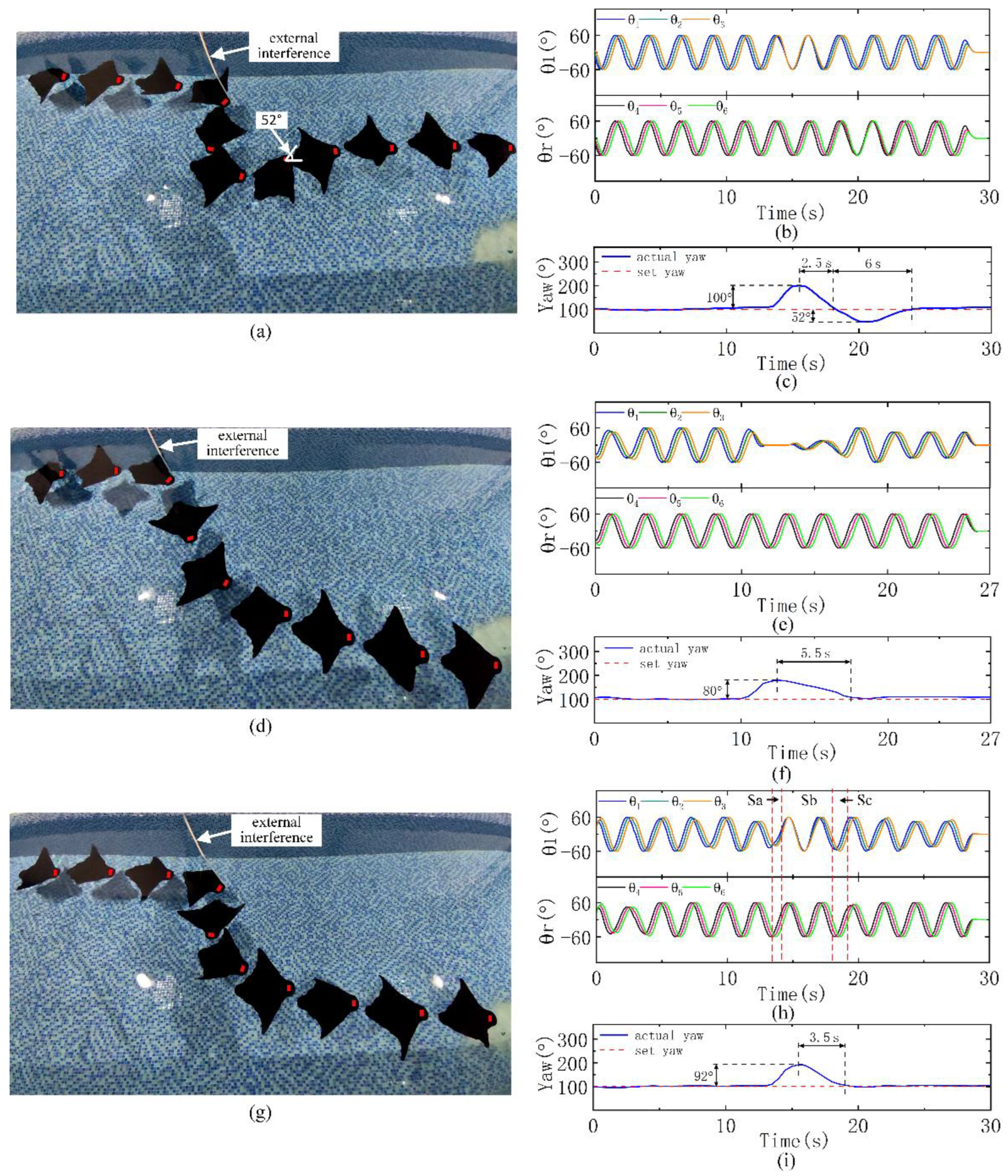
The course adjustment using only the phase difference is performed first (Figure 5a). After interference, the course deviates from the starting course by approximately 100°. The robot adjusts the course using the phase difference between the pectoral fins (Figure 5b). It takes only 2.5 s to adjust back to the starting course. The yaw angle rate during the adjustment process is 40°/s. However, due to the fast yaw angle rate and the time required for the phase transition, after the first adjustment back to the initial course, there is an overshoot of 52%. Then, the course is readjusted to the initial course. The adjustment time from the maximum deviation of the course to the adjustment back to the initial course is 8.5 s (Figure 5c). Due to the limited width of the pool, to avoid colliding with the wall during the adjustment process, in the interference test relying on the amplitude difference, we applied a slightly lower intensity interference (Figure 5d). After interference, the course deviates from the starting course by approximately 80°. The robot adjusts the course using amplitude difference between the pectoral fins (Figure 5e). This method takes 5.5 s to adjust back to the starting course, and the yaw angle rate during adjustment is 14.5°/s. Due to the slow adjustment speed, there is no overshoot. After adjusting back to the initial course, the robot continues to swim forward (Figure 5f). Similar to biologic rays, the phase difference mode has more advantages in yaw mobility and yaw radius. However, due to its fast yaw angle rate and the output transition time, there will be a large overshoot, resulting in a longer adjustment time than when relying on the asymmetric amplitude mode. Inspired by these two yaw modes, we combine them to retain the yaw rapidity and reduce the overshoot. Similarly, for the experiment adjusting the course in combination (Figure 5g), we apply a course interference of approximately 92°. When the course deviation is greater than 30°, the robot relies on asymmetric amplitude adjustment (Sa and Sc in Figure 5h); when the course deviation is less than 30°, the robot relies on asymmetric amplitude adjustment (Sb in Figure 5h). This method takes 3.5 s to adjust back to the initial course. The yaw angle rate in the adjustment process is 26.3°/s (Figure 5i), which is slower than the 40°/s relying on the phase difference method. However, this method avoids overshoot while ensuring the yaw angle rate, and the overall adjustment time is greatly reduced compared with the 8.5 s relying on the amplitude difference method. The yaw angle rate is also greatly improved compared with 14.5°/s in the amplitude difference mode, which verifies the rapidity and stability of the yaw of the robot under external interference using the combined mode control strategy.

3.6. Course Adjustment Experiments

In addition to verifying the course adjustment ability of the robot under interference, we also try to verify the performance of the robot in actively adjusting the course to ensure its working ability in a complex environment. In this part of the experiments, the turning performance difference between the phase difference mode and the combined mode is compared.

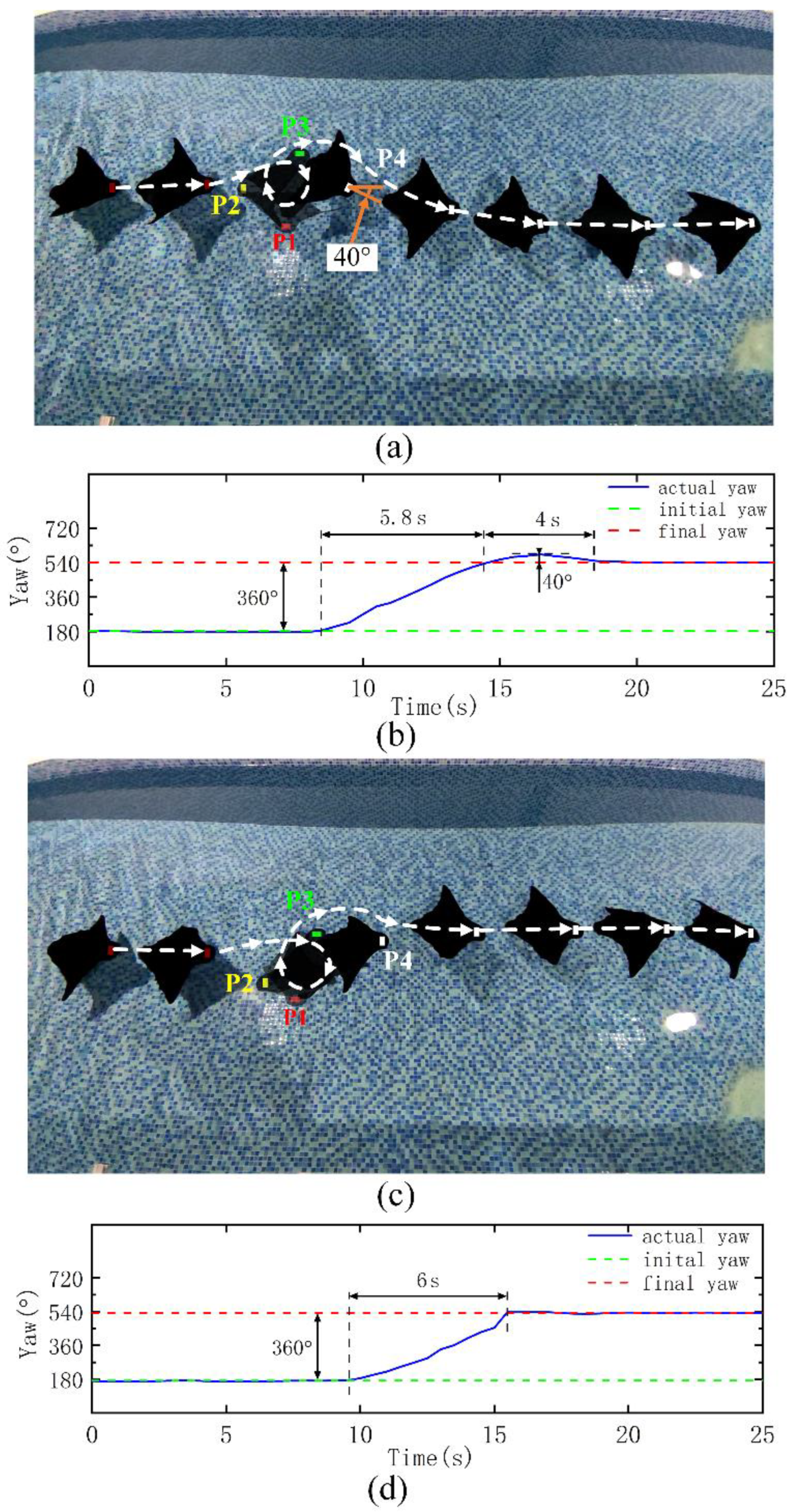
We try to make the robot turn 360° to the right under the normal forward swimming mode and then restore the forward swimming mode. The frame pictures labeled P1, P2, P3 and P4 in Figure 6a, c are the typical pose diagrams of the robot turning 90°, 180°, 270°, 360°. For convenience, when the robot turns right, its course angle continues to accumulate. After turning right for one cycle, the course angle increases 360°. Relying only on the phase difference to adjust the course, it takes 5.8 s to turn for one cycle, and the yaw angle rate is 62°/s. As in the course interference experiment, there will be an overshoot of approximately 40° after one cycle of turning and a final readjustment to the starting course. The adjustment time of the whole process is 9.8 s (Figure 6b). It takes 6s to turn 360° to the right by relying on the combined mode, and the yaw angle rate is 60°/s. Compared with the phase difference mode, the yaw angle rate is hardly reduced and will not produce an overshoot. The robot can stably return to the initial course, and the adjustment time in the whole process is reduced (Figure 6d). Experiments show that the combined mode has almost the same rapidity and no overshoot compared with the phase difference mode.

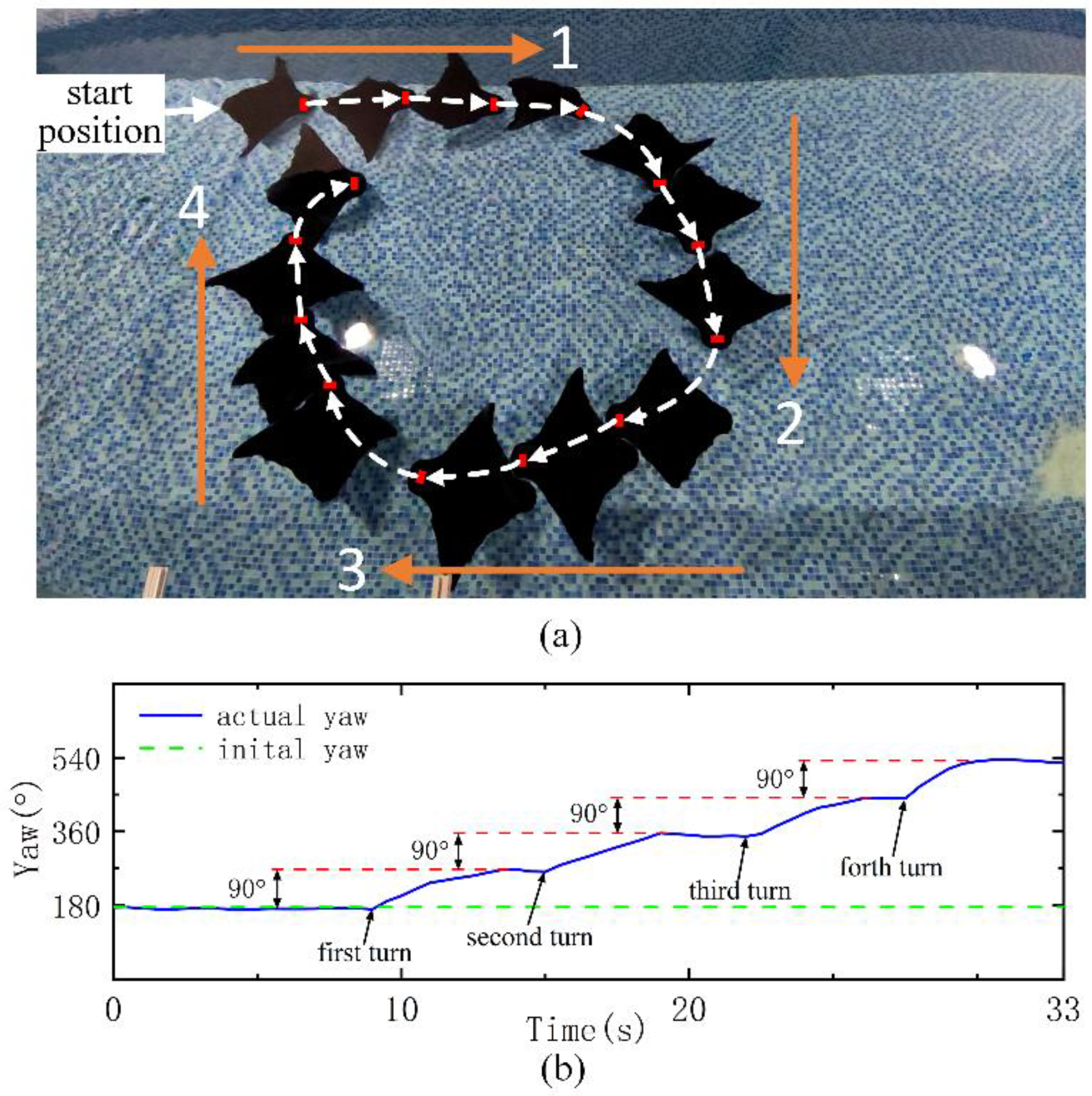
Finally, we also try to verify the ability of the robot to turn continuously (Figure 7a) as the robot follows a preset trajectory. In order to test the ability of the robot to move continuously in a narrow small area, we selected a certain length of the pool instead of using the whole length. First, the robot swims with the azimuth angle set in direction 1 for 8 s. The robot then turns 90° right, swims forward with the azimuth angle set in direction 2 for 6 s, and then turns 90° right. The swimming times of the robot along directions 3 and 4 are 8 s and 6 s, respectively (Figure 7b). Through four turns of 90°, the robot completes the path trajectory along directions 1, 2, 3 and 4 like a rectangle. Due to the limited width of the pool, the robot swims in each direction for a short time, but it is not difficult to see that the robot still has excellent adjustment ability in continuous turning performance, which verifies the effectiveness of the control strategy.

3.7. Discussion

Here, a control strategy based on amplitude and phase differences is proposed. Through a series of experiments, the maneuverability of the robot under external interference and course adjustment is verified. Compared with the existing manta ray robots in the Table 1, the proposed robot has significant comprehensive maneuver performance. First, the robot with proposed control strategy has good ability to resist external interference, which is relatively lacking in previous research. Second, combined with the yaw mode and characteristics of organisms, the proposed control strategy not only ensures the yaw angle rate of robot, but also avoids the overshoot when reaching the target course, and realizes the maximum yaw angle rate of 62°/s. Finally, through the rectangular swimming experiment, the ability of continuous maneuvering of the robot in complex environment is verified, which lays a foundation for the application in practical scenes.

The proposed robot has certain mobility, but the experiment carried out is relatively simple. On the one hand, there is a certain gap between the artificial interference and the actual application scene. On the other hand, only one interference is applied without multiple times, and the experimental conditions are ideal. In addition, in the yaw process, only one index of yaw angle rate is concerned, and the stability in the yaw process is not concerned. In the experiment, due to the rapid change of thrust on both sides, the yaw stability of the robot is not good. In general, the good mobility of the robot is realized, which lays a good foundation for the research of autonomous decision-making and obstacle avoidance.

4. Conclusions

In this paper, referring to the amplitude transition equation of a phase oscillator model, an expected phase difference transition equation is introduced to realize the smooth transition of the expected phase difference. Based on this, the problem of the output not being smooth due to the change in the expected phase difference is avoided. Inspired by the biological yaw modes, after simulation verification, open-loop experiments of the two yaw modes are carried out, and the characteristics of the two yaw modes are compared. The yaw angle rate based on the phase difference is faster, and the continuity of the yaw angle rate change based on the amplitude difference is better. Based on the characteristics of these two yaw modes, on the basis of realizing closed-loop depth control, we adopt the combined closed-loop course control strategy of adjusting the course using the phase difference when the course deviation is greater than 30° and adjusting using the amplitude difference when the deviation is less than 30°. First, we verify the advantages of the combined control mode through a course interference experiment, which not only retains the yaw rapidity but also avoids overshoot, and the overall adjustment time is the lowest. Then, in an active course adjustment experiment, the combined control strategy still has more advantages than the single phase difference mode. Finally, the high-maneuverability of the robot is verified through a rectangular trajectory swimming experiment.

In future work, we will pay more attention to the rolling stability of the robot during the yaw process to ensure the stability of the robot while realizing rapid and stable yaw.