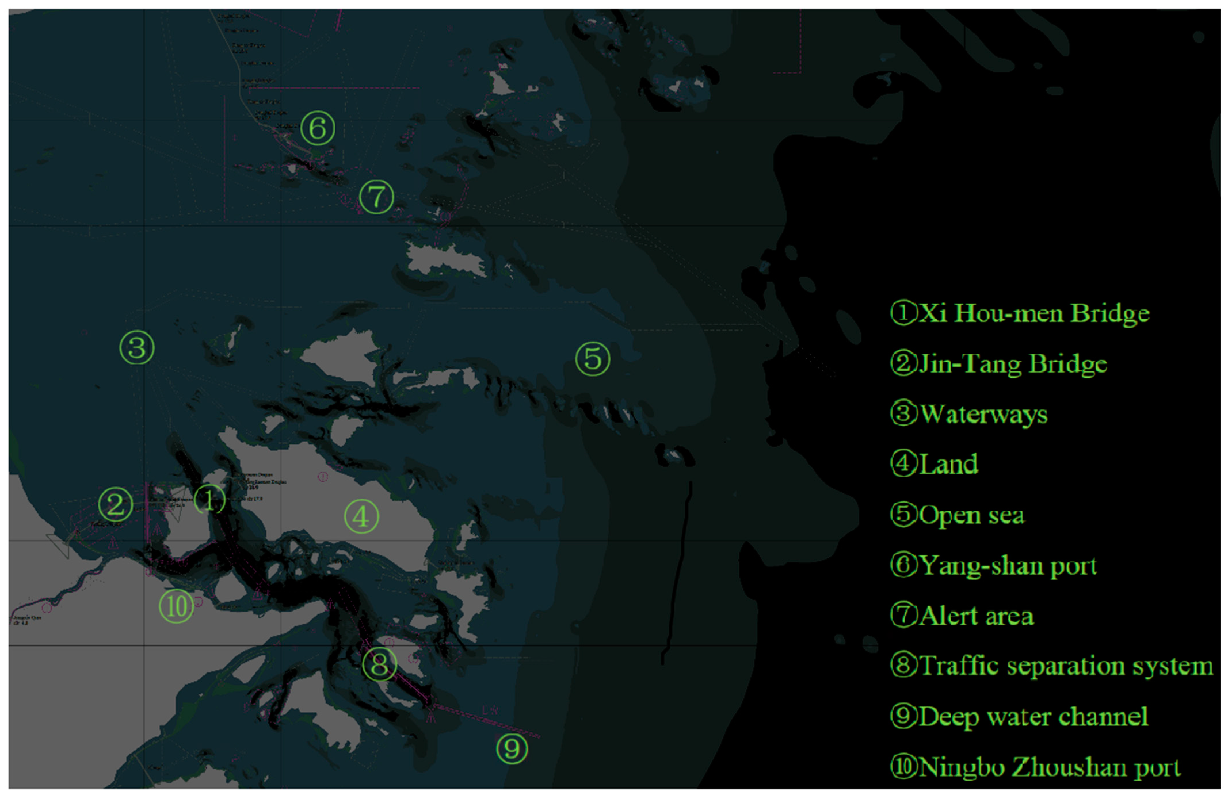
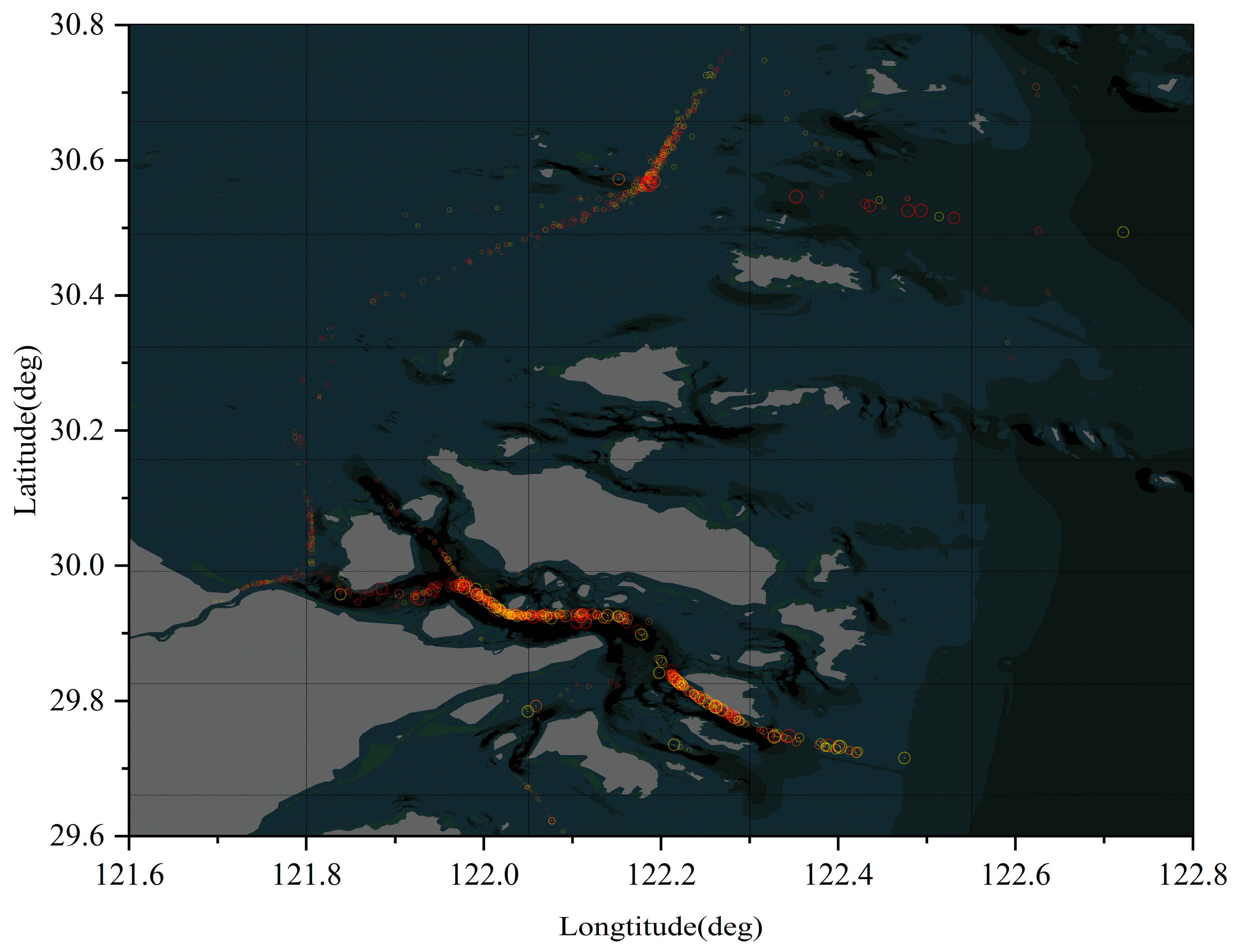
Figure 1.
The study area for collision risk assessment.
Figure 1.
The study area for collision risk assessment.
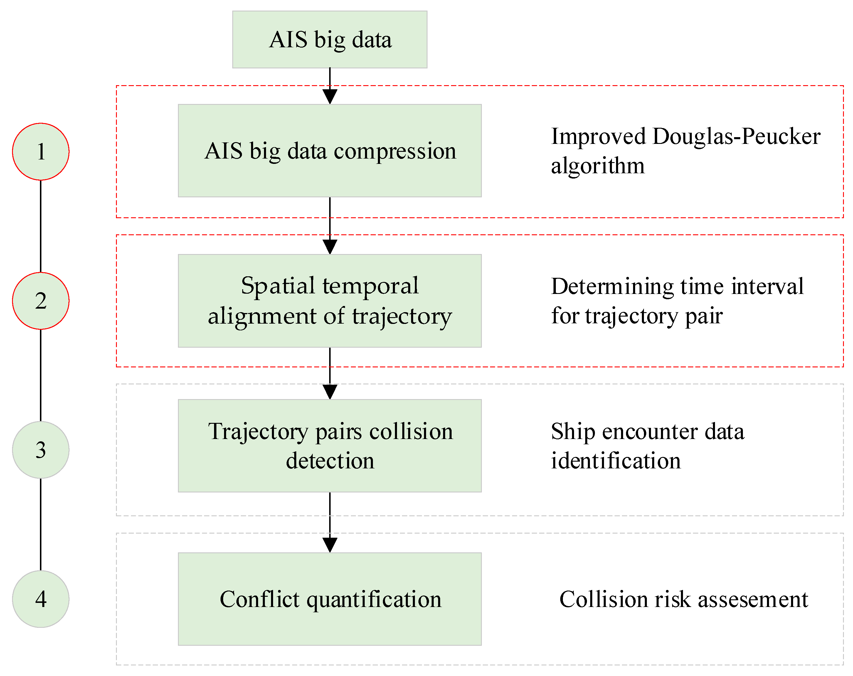
Figure 2.
Framework of collision risk assessment.
Figure 2.
Framework of collision risk assessment.
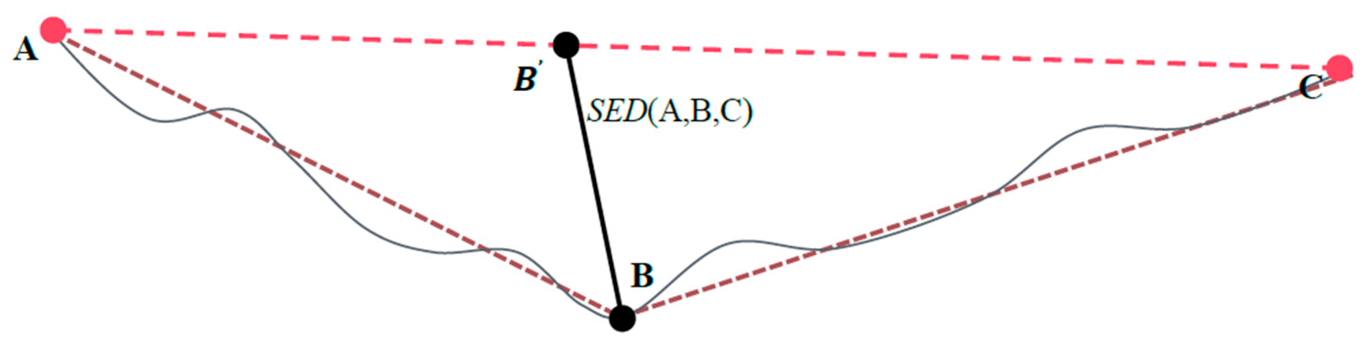
Figure 3.
Synchronous Euclidean Distance. Where segment is the successive track points after compressing and point list is the successive actual location of the track. Point is the generated synchronization point. is the Synchronous Euclidean distance between the point and . The velocity of the Synchronized point B is , the time is and the course is .
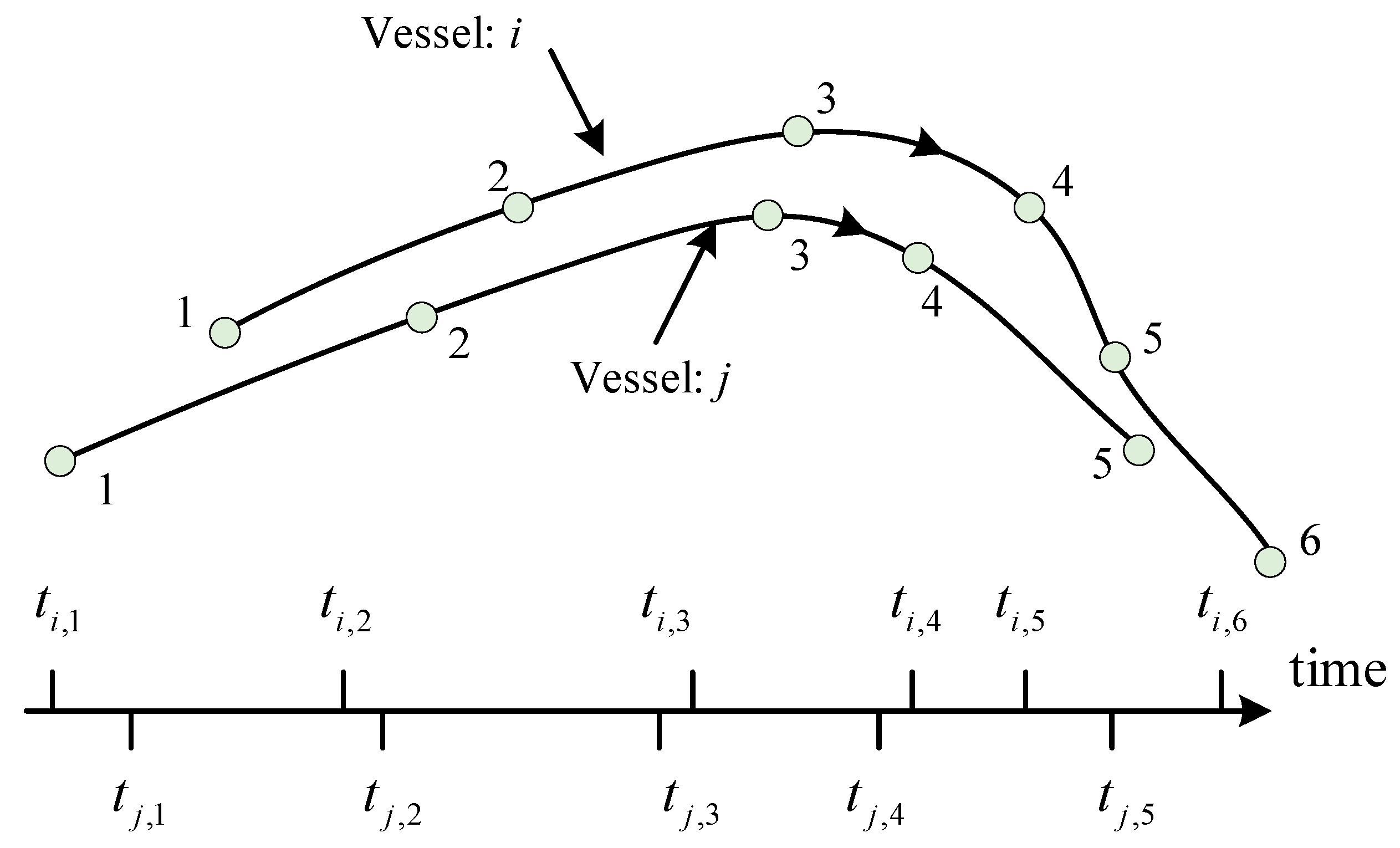
Figure 4.
Determining the time interval from trajectory pairs.
Figure 4.
Determining the time interval from trajectory pairs.
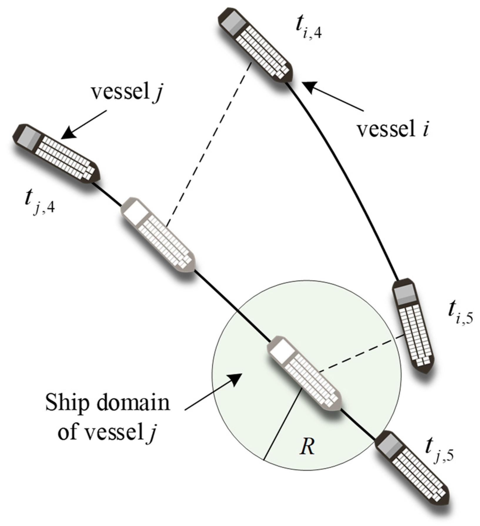
Figure 5.
A conflict example for trajectories pairs.
Figure 5.
A conflict example for trajectories pairs.
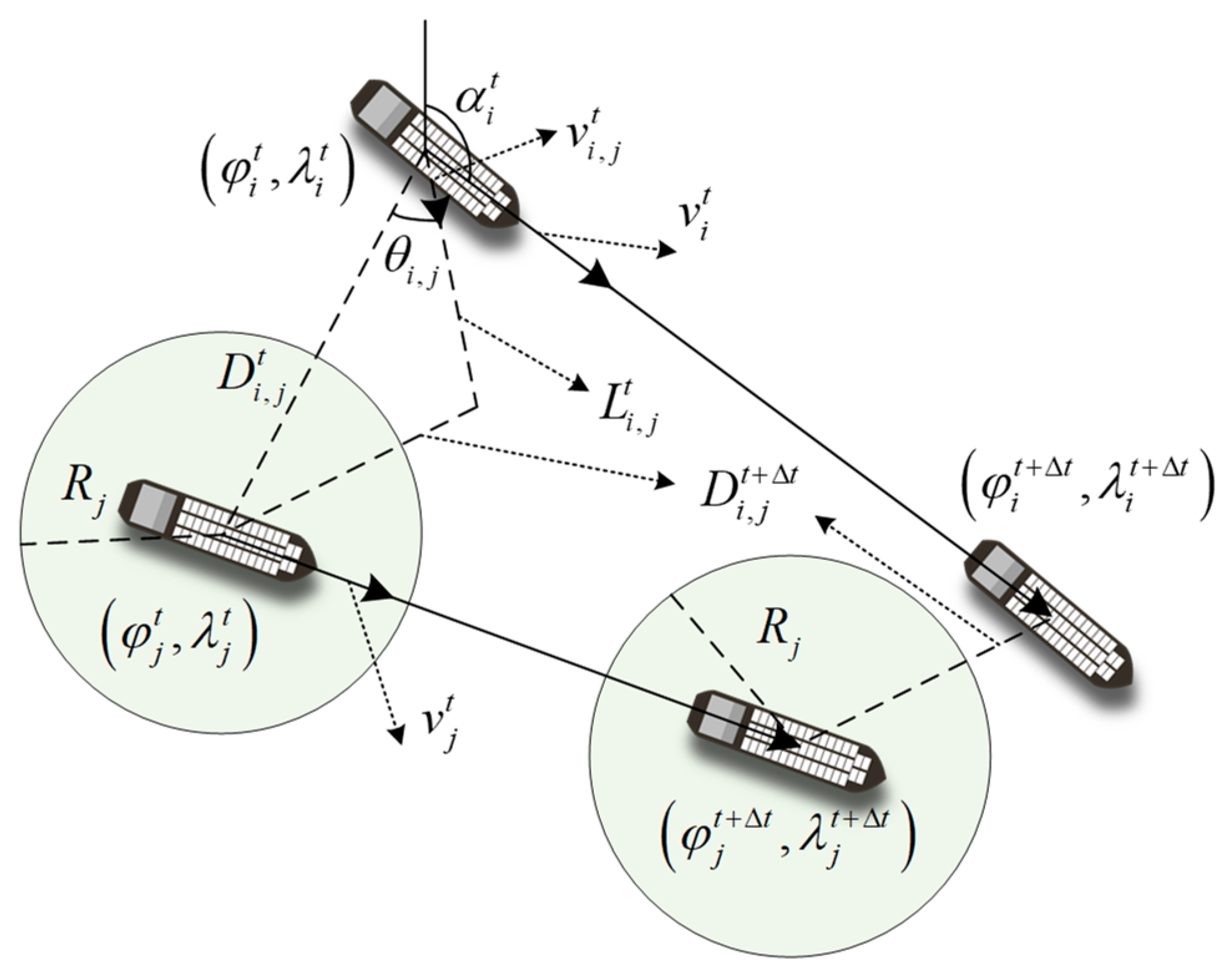
Figure 6.
Relative motion of vessel pair at a time interval and ship conflicts.
Figure 6.
Relative motion of vessel pair at a time interval and ship conflicts.
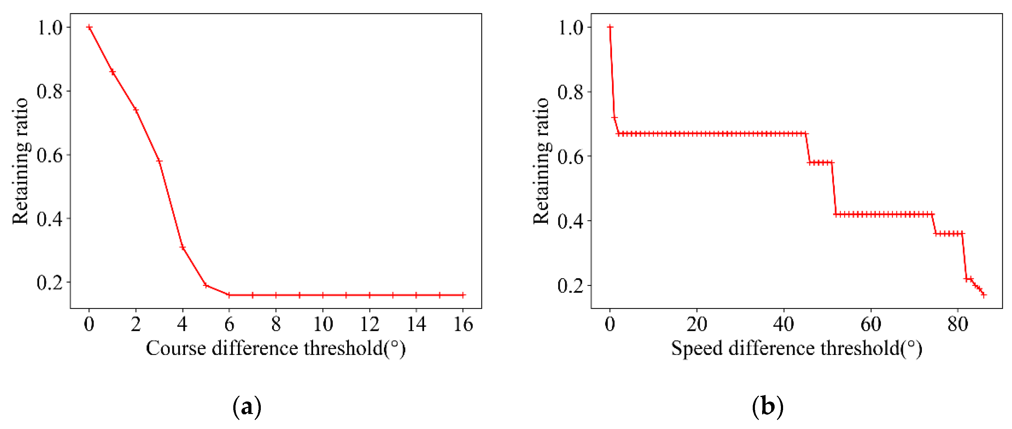
Figure 7.
The relationship between retaining ratio and speed constraint or course constraint. (a) is the relationship between the retaining ratio and course constraint when the speed constraint is 87 and the threshold of the Euclidean distance is 100 times; (b) is the relationship between the retaining ratio and speed threshold when the course threshold is 27 and the threshold of the Euclidean distance is 100 times.
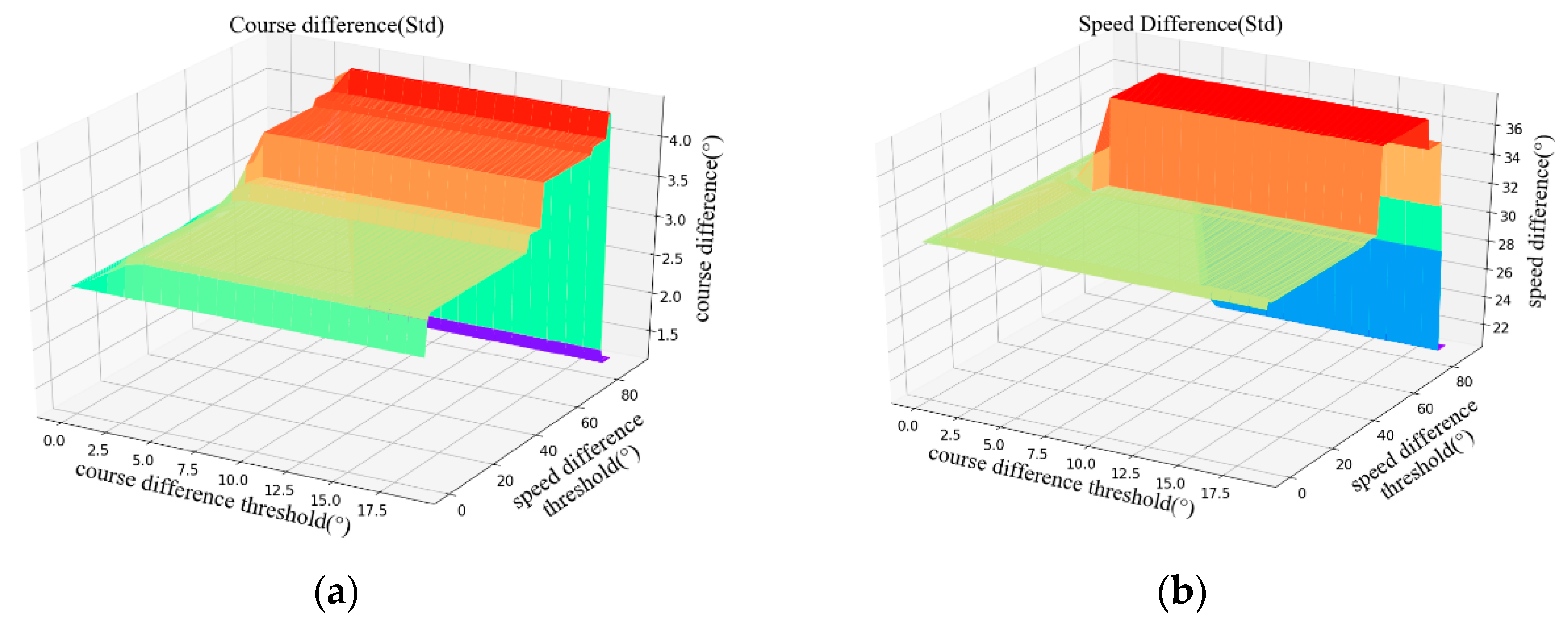
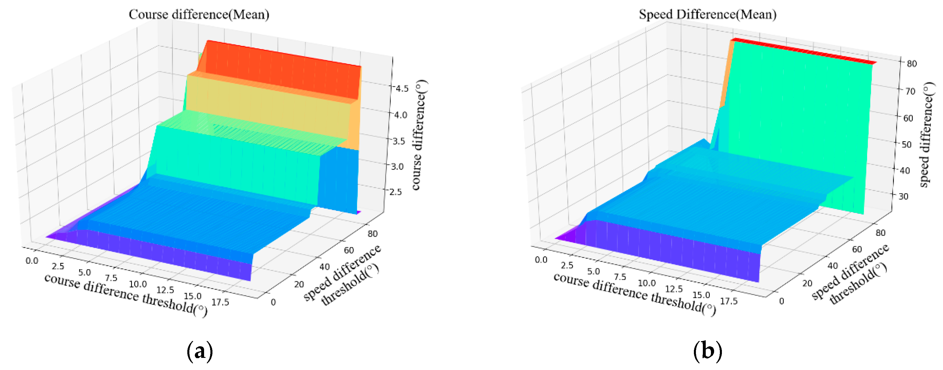
Figure 8.
Correlation between the standard error of the course difference threshold, the speed difference threshold, and the course difference or speed mean difference. (a) shows the course difference; (b) shows the speed difference.
Figure 8.
Correlation between the standard error of the course difference threshold, the speed difference threshold, and the course difference or speed mean difference. (a) shows the course difference; (b) shows the speed difference.
Figure 9.
Correlation between the course difference threshold, speed difference threshold, and the mean error of course difference or speed difference. (a) shows the course difference; (b) shows the speed difference.
Figure 9.
Correlation between the course difference threshold, speed difference threshold, and the mean error of course difference or speed difference. (a) shows the course difference; (b) shows the speed difference.
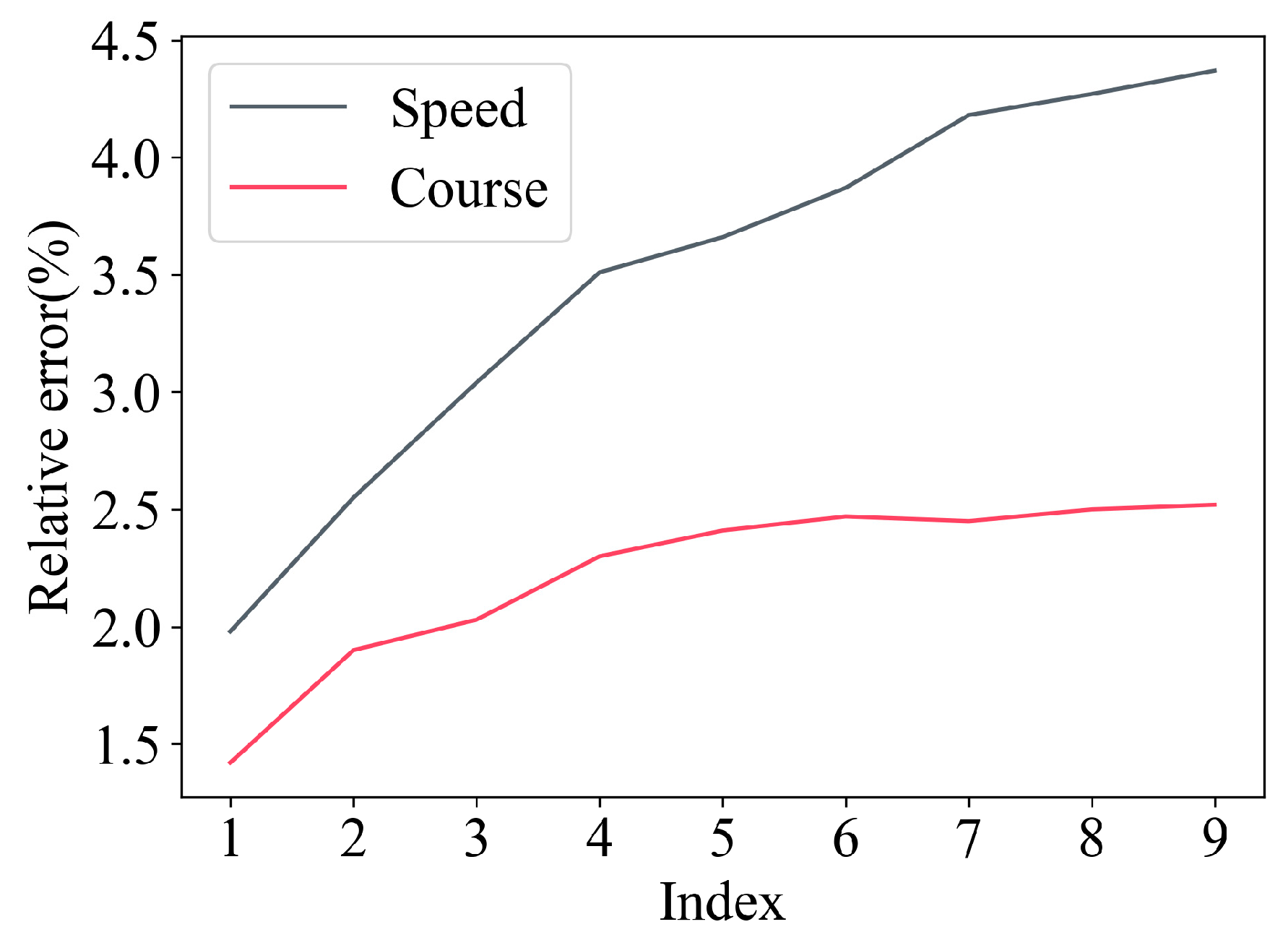
Figure 10.
The relative error between Synchronous Euclidean Distance error of speed and course of RDP and MCDP.
Figure 10.
The relative error between Synchronous Euclidean Distance error of speed and course of RDP and MCDP.
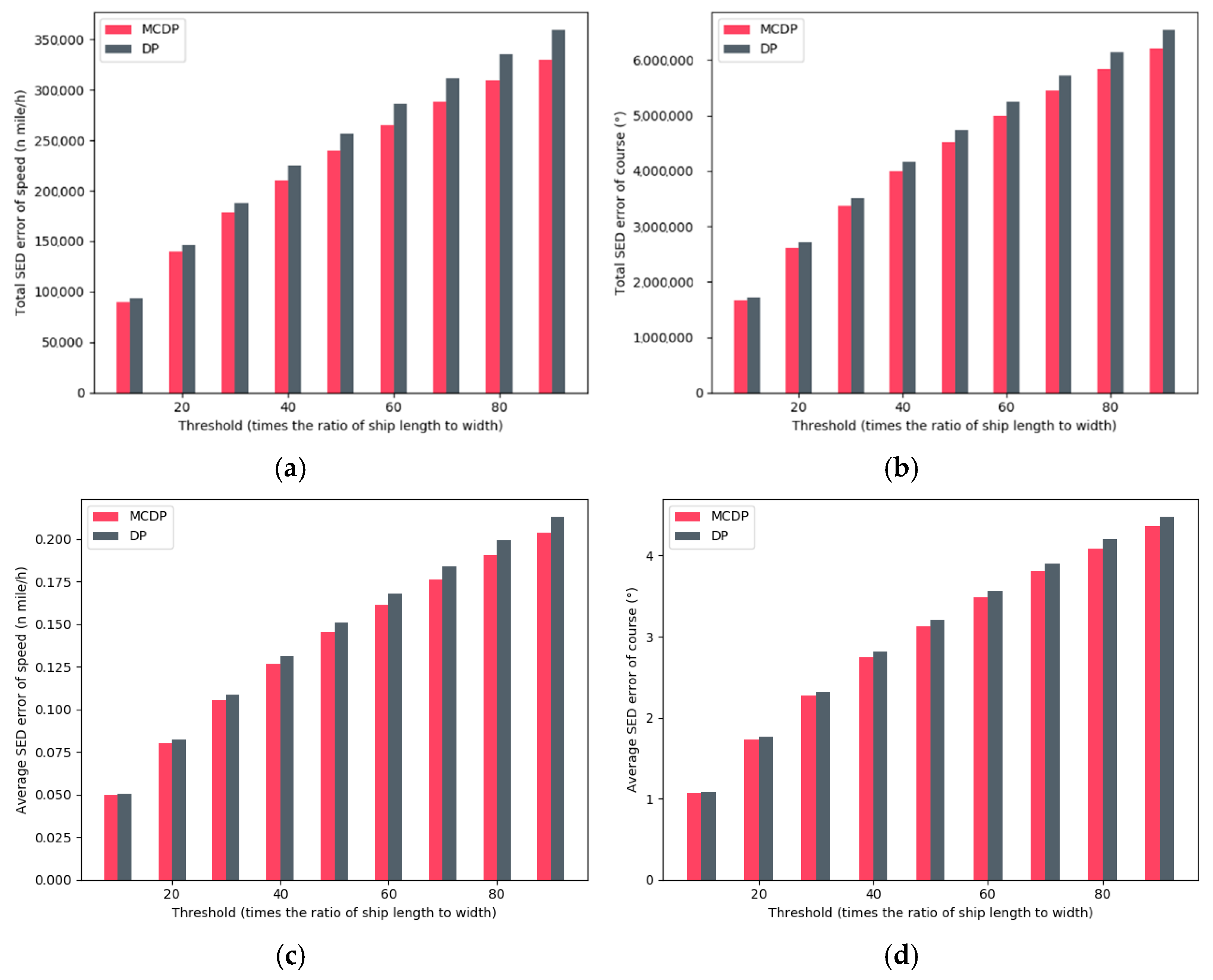
Figure 11.
Comparison between Synchronous Euclidean Distance error of speed and course of RDP and MCDP. (a–d) show the total SED error of speed, total SED error of course, average SED error of speed, and average SED error of course, respectively.
Figure 11.
Comparison between Synchronous Euclidean Distance error of speed and course of RDP and MCDP. (a–d) show the total SED error of speed, total SED error of course, average SED error of speed, and average SED error of course, respectively.
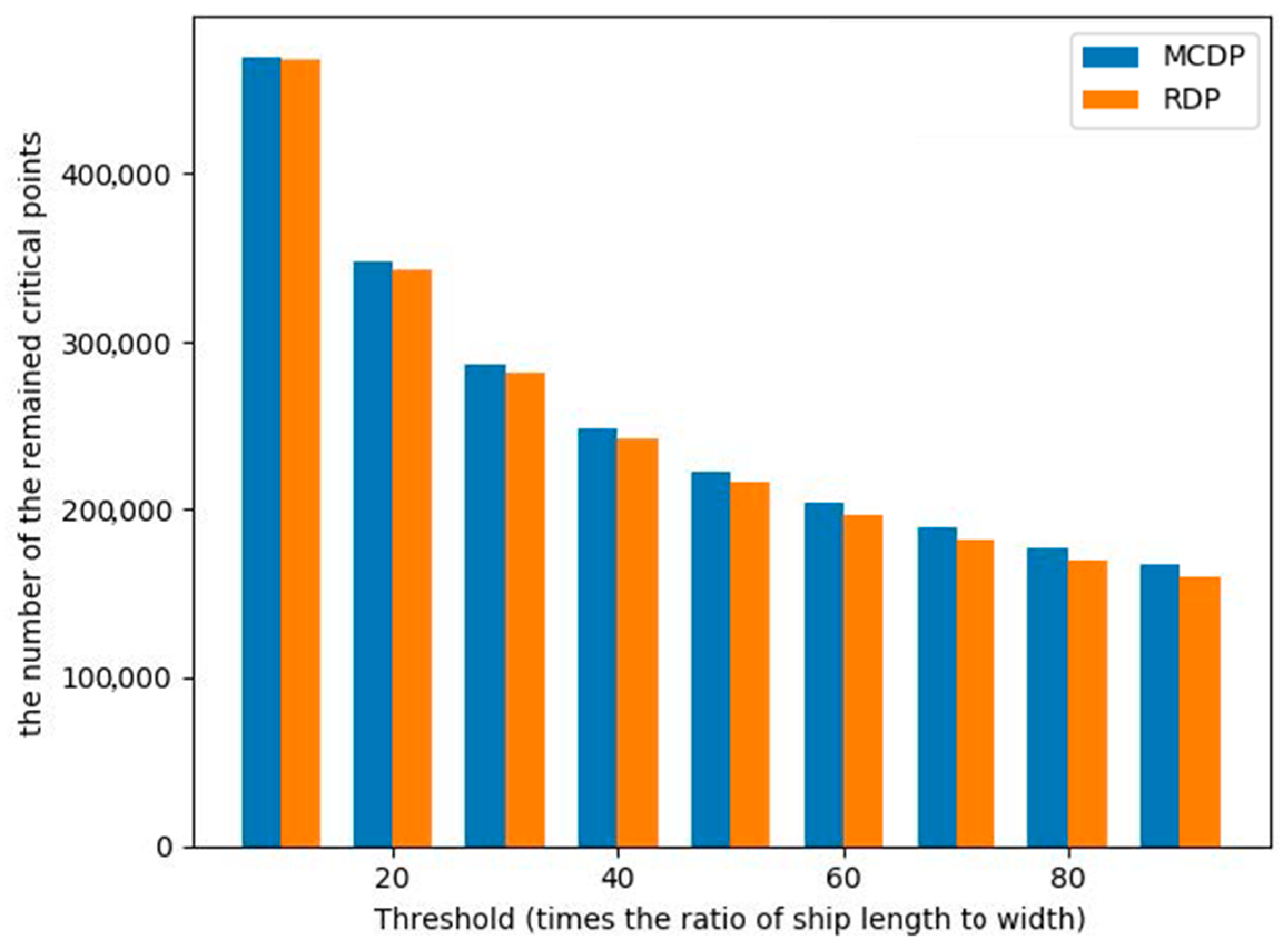
Figure 12.
Comparison between MCDP and RDP.
Figure 12.
Comparison between MCDP and RDP.
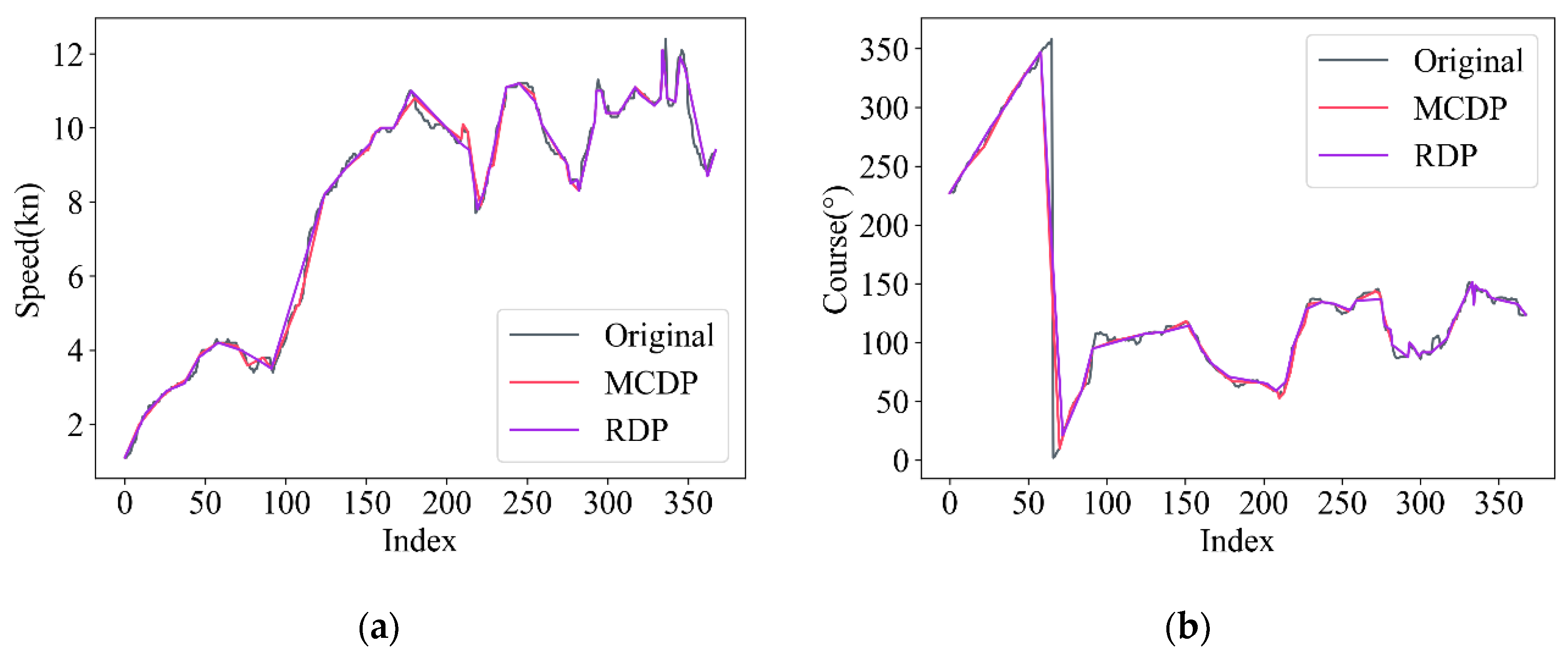
Figure 13.
Charts comparing with the RDP algorithm and the MCDP algorithm (Our algorithm). (a) is the velocity simplification comparison with RDP, original, and MCDP; (b) is the course simplification comparison with RDP, original, and MCDP. The threshold was set as 50 times the ship length to width.
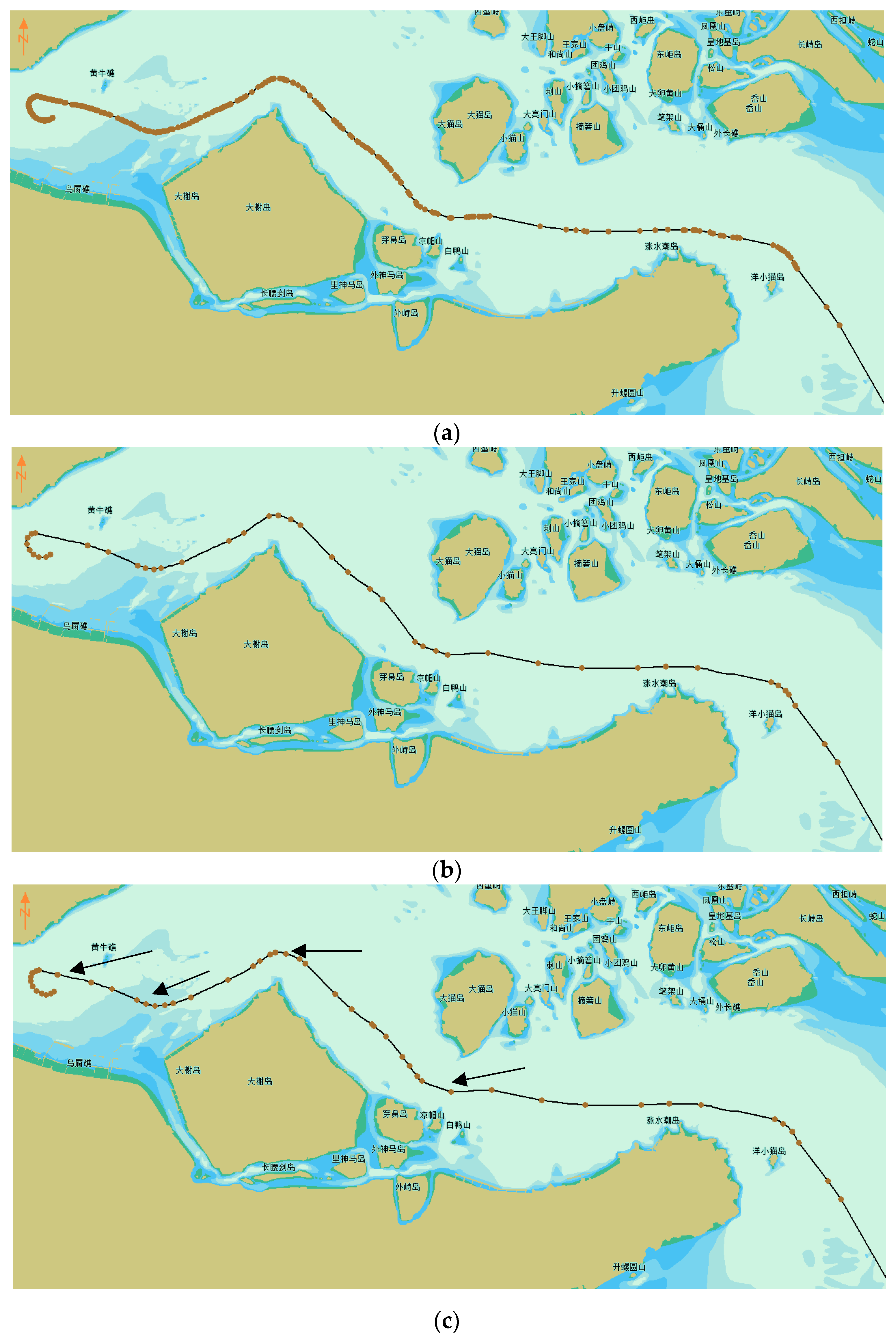
Figure 14.
Compression results of vessel trajectory in the parallel experiment. (a) Original trajectory; (b) The simplified trajectory by RDP; (c) The simplified trajectory by MCDP.
Figure 14.
Compression results of vessel trajectory in the parallel experiment. (a) Original trajectory; (b) The simplified trajectory by RDP; (c) The simplified trajectory by MCDP.
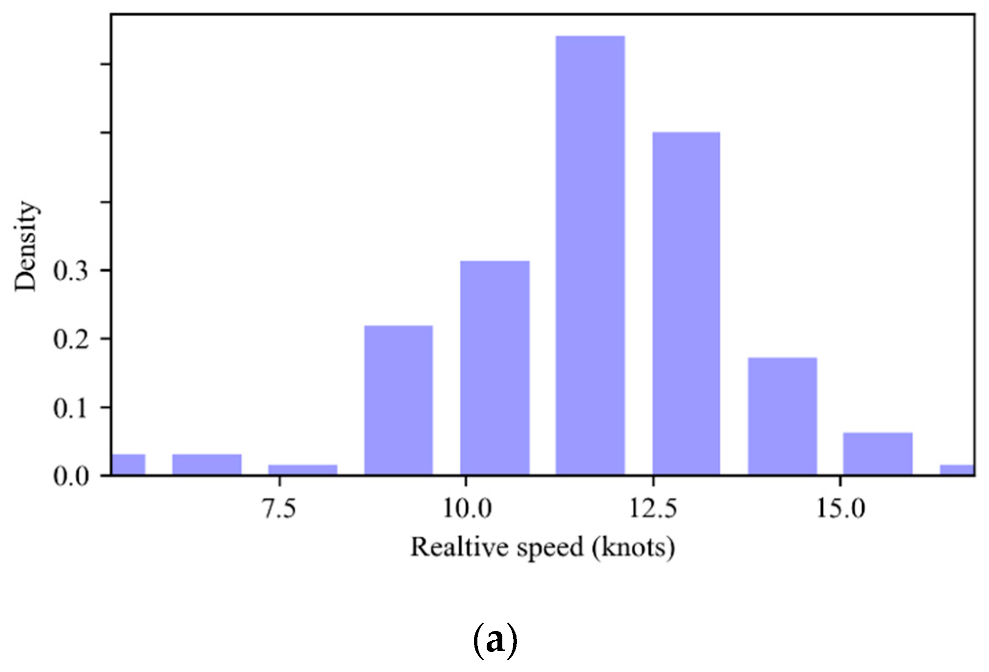
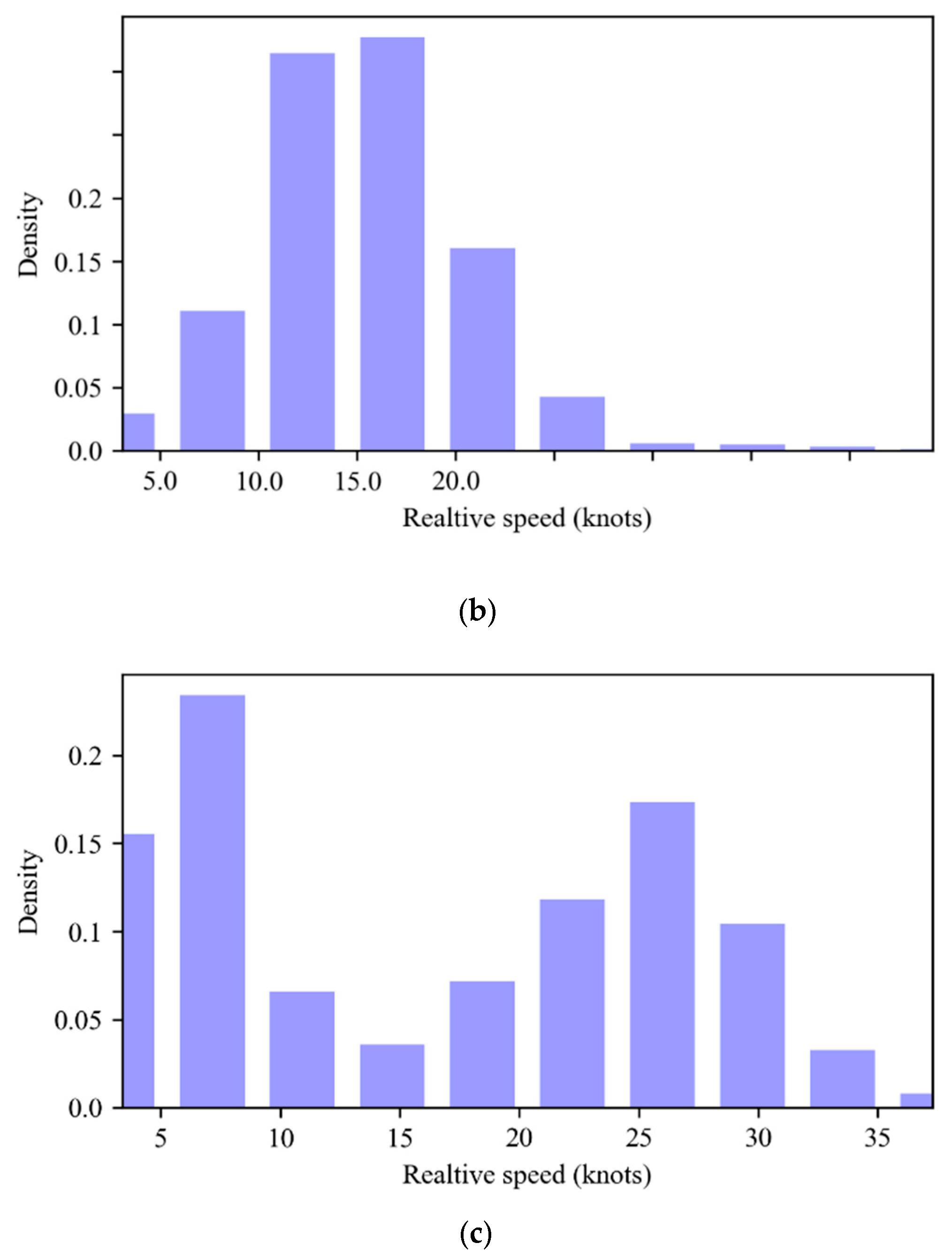
Figure 15.
Relative speed distribution for vessels involving in different conflicts. (a) Head-on conflict; (b) Crossing conflict; (c) Overtaking conflict.
Figure 15.
Relative speed distribution for vessels involving in different conflicts. (a) Head-on conflict; (b) Crossing conflict; (c) Overtaking conflict.
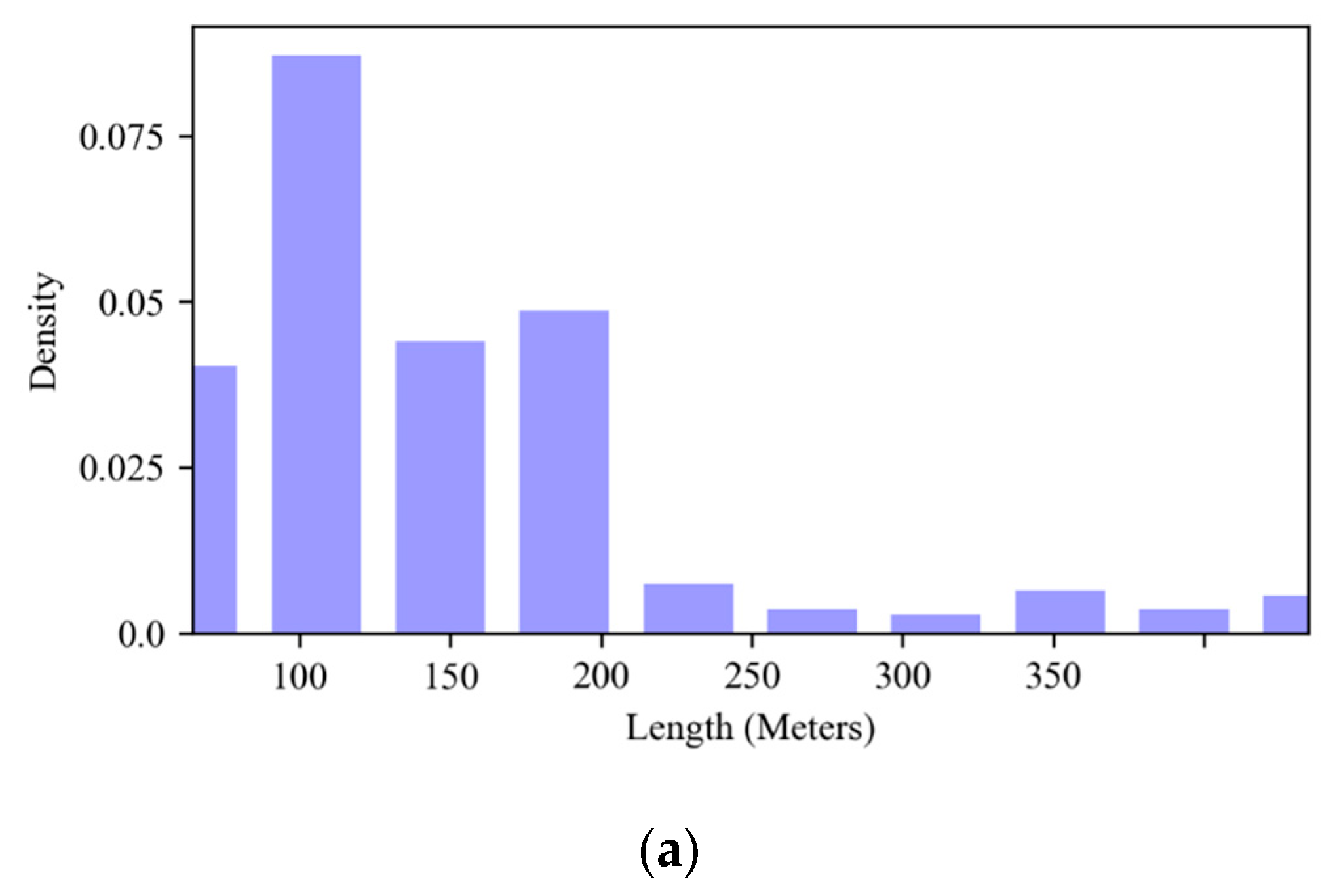
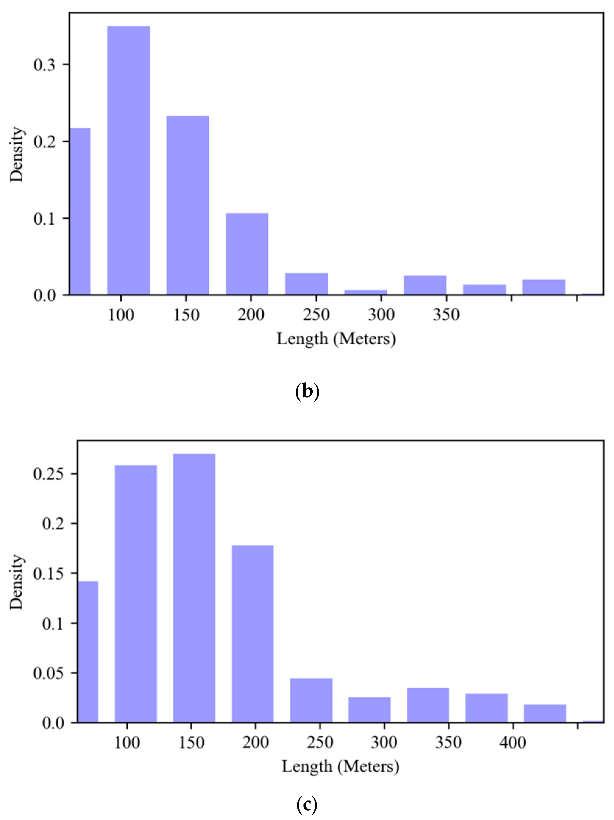
Figure 16.
Length distribution for vessels involved in different conflicts. (a) Head-on conflict; (b) Crossing conflict; (c) Overtaking conflict.
Figure 16.
Length distribution for vessels involved in different conflicts. (a) Head-on conflict; (b) Crossing conflict; (c) Overtaking conflict.
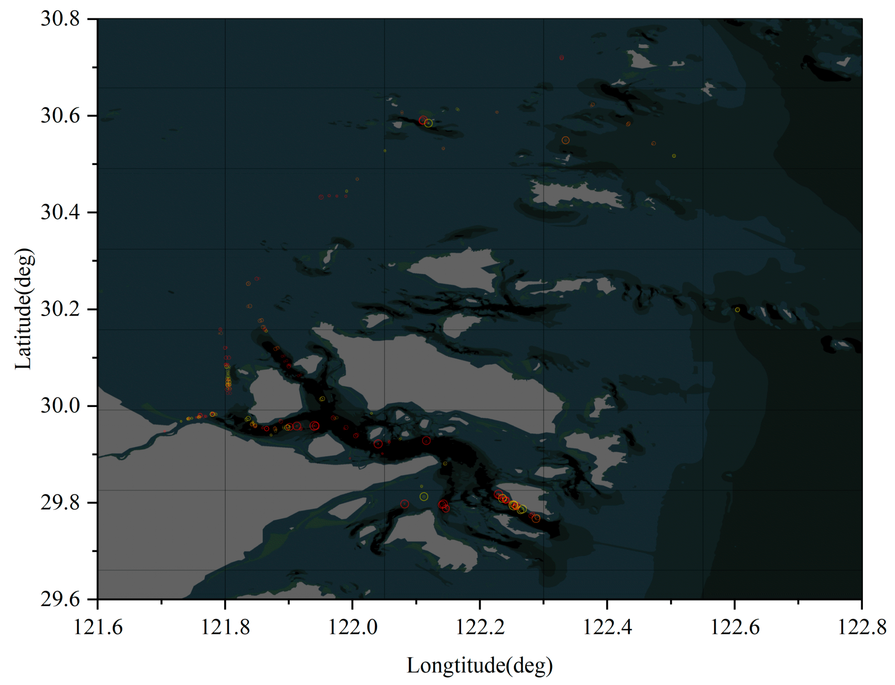
Figure 17.
Spatio-temporal distribution of head-on conflicts.
Figure 17.
Spatio-temporal distribution of head-on conflicts.
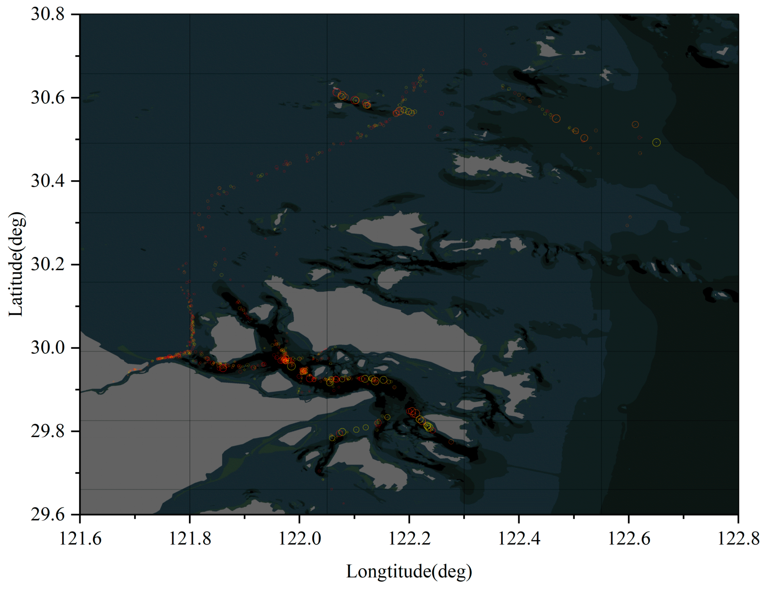
Figure 18.
Spatio-temporal distribution of crossing conflicts.
Figure 18.
Spatio-temporal distribution of crossing conflicts.
Figure 19.
Spatio-temporal distribution of overtaking conflicts.
Figure 19.
Spatio-temporal distribution of overtaking conflicts.
Table 1.
Description of the measurement.
Table 1.
Description of the measurement.
| Measurement | Description | Unit |
|---|
| SEDtotv | Total speed synchronization error of trajectories | Knots |
| SEDavgv | Average speed synchronization error of trajectories | Knots |
| SEDtotc | Total course synchronization error of trajectories | Degree |
| SEDavgc | Average course synchronization error of trajectories | Degree |
| THR | Threshold (times the ratio of ship length to width) | None |
Table 2.
Quantity analysis for comparison between the existing method and proposed method.
Table 2.
Quantity analysis for comparison between the existing method and proposed method.
| THR | RDP | MCDP | Deleted Incorrectly |
|---|
| Remained | Ratio (%) | Remained | Ratio (%) |
|---|
| 10 | 467,451 | 0.577976077 | 469,425 | 0.576193911 | 1974 |
| 20 | 343,302 | 0.690060227 | 347,703 | 0.686086918 | 4401 |
| 30 | 281,684 | 0.745690165 | 287,016 | 0.740876331 | 5332 |
| 40 | 242,889 | 0.780715051 | 248,949 | 0.775243964 | 6060 |
| 50 | 216,143 | 0.804861864 | 222,759 | 0.79888881 | 6616 |
| 60 | 196,856 | 0.822274546 | 203,506 | 0.816270795 | 6650 |
| 70 | 181,883 | 0.835792463 | 188,885 | 0.829470921 | 7002 |
| 80 | 170,002 | 0.846518863 | 177,063 | 0.840144054 | 7061 |
| 90 | 160,180 | 0.855386357 | 167,173 | 0.84907294 | 6993 |
Table 3.
Speed loss of RDP and MCDP on the dataset with different thresholds.
Table 3.
Speed loss of RDP and MCDP on the dataset with different thresholds.
| THR | RDP | MCDP |
|---|
| SEDtotv | SEDavgv | SEDtotv | SEDavgv |
|---|
| 10 | 93,320.9337 | 0.0506 | 90,102.9013 | 0.0496 |
| 20 | 146,309.7629 | 0.0824 | 139,549.0754 | 0.0803 |
| 30 | 188,422.1134 | 0.1085 | 178,265.4737 | 0.1052 |
| 40 | 224,651.3745 | 0.1312 | 210,409.2579 | 0.1266 |
| 50 | 256,911.2068 | 0.15082 | 239,676.8059 | 0.1453 |
| 60 | 285,895.6688 | 0.1681 | 265,157.2075 | 0.1616 |
| 70 | 311,667.0748 | 0.1840 | 288,211.9025 | 0.1763 |
| 80 | 335,843.8289 | 0.1992 | 309,908.0217 | 0.1907 |
| 90 | 359,218.8910 | 0.2129 | 329,731.6156 | 0.2036 |
Table 4.
Course loss of RDP and MCDP on the dataset with different thresholds.
Table 4.
Course loss of RDP and MCDP on the dataset with different thresholds.
| THR | RDP | MCDP |
|---|
| SEDtotc | SEDavgc | SEDtotc | SEDavgc |
|---|
| 10 | 1,711,254.8141 | 1.0810 | 1,663,394.0128 | 1.0656 |
| 20 | 2,713,959.2632 | 1.7590 | 2,620,121.4988 | 1.7256 |
| 30 | 3,503,489.6310 | 2.3169 | 3,373,388.1781 | 2.2699 |
| 40 | 4,174,016.6652 | 2.8159 | 3,990,199.7671 | 2.7510 |
| 50 | 4,740,253.5191 | 3.2101 | 4,524,679.0714 | 3.1326 |
| 60 | 5,245,404.4085 | 3.5704 | 5,001,570.1720 | 3.4821 |
| 70 | 5,716,247.3330 | 3.8996 | 5,441,852.0286 | 3.8040 |
| 80 | 6,134,831.4963 | 4.1966 | 5,837,147.1061 | 4.0917 |
| 90 | 6,540,768.7990 | 4.4750 | 6,211,981.4299 | 4.3621 |
Table 5.
Comparison of collision frequency in different duty periods.
Table 5.
Comparison of collision frequency in different duty periods.
| Collision Type | Head On | Crossing | Overtaking | Overall |
|---|
| First officer | | | | |
| Second officer | | | | |
| Third officer | | | | |
Table 6.
Comparison of collision frequency in different encounter situations.
Table 6.
Comparison of collision frequency in different encounter situations.
| Collision Type | Mean/Day | Std/Day | F | p-Value |
|---|
| Head-on | | | | |
| First officer | | | 5.92 | 0.008 |
| Second officer | | | | |
| Third officer | | | | |
| Crossing | | | | |
| First officer | | | 2.68 | 0.089 |
| Second officer | | | | |
| Third officer | | | | |
| Overtaking | | | | |
| First officer | | | 3.69 | 0.040 |
| Second officer | | | | |
| Third officer | | | | |


