Modeling of Ship DC Power Grid and Research on Secondary Control Strategy


Abstract
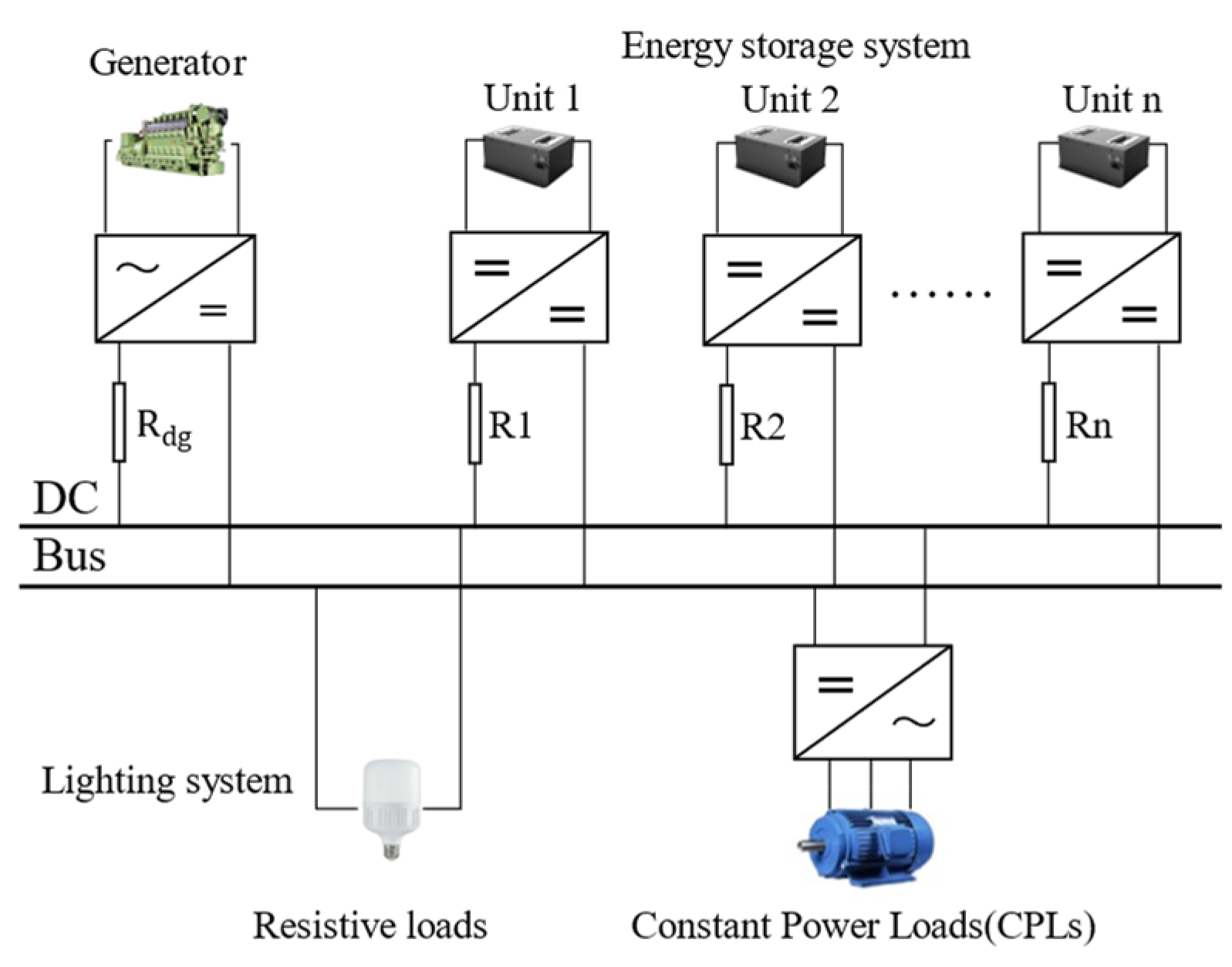
:1. Introduction
2. Converter and Its Controller
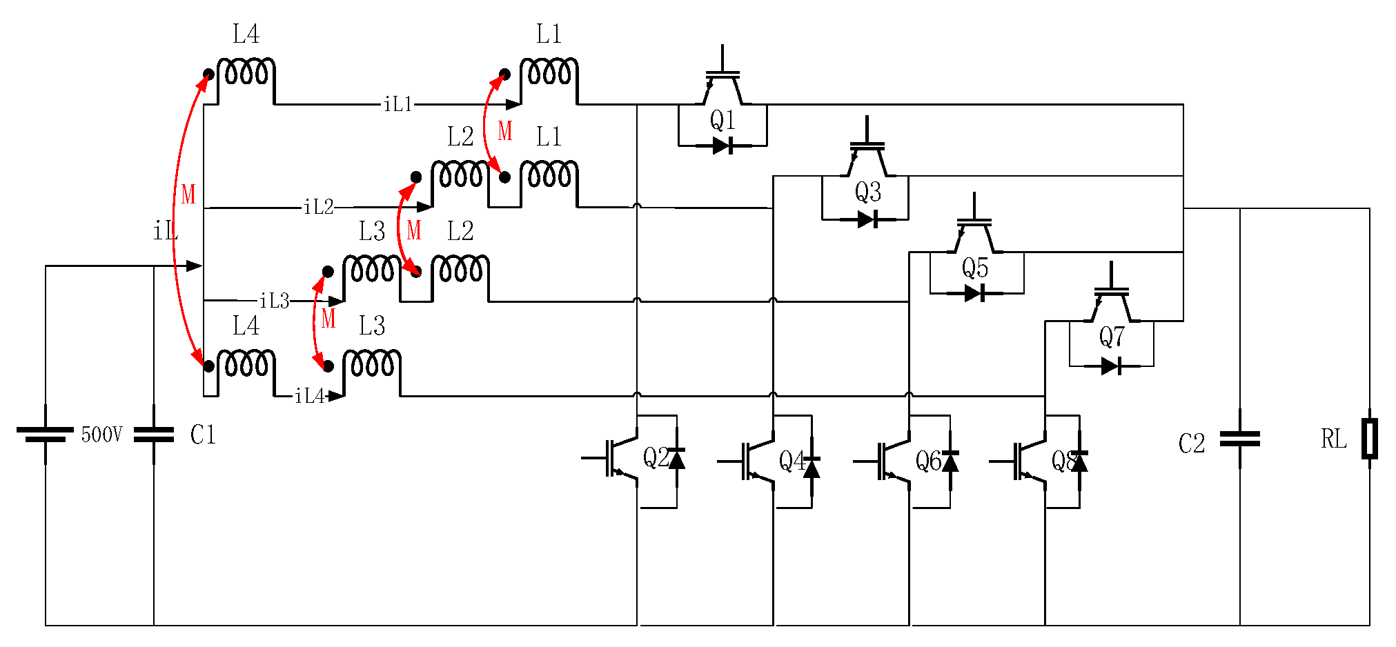
2.1. Converter
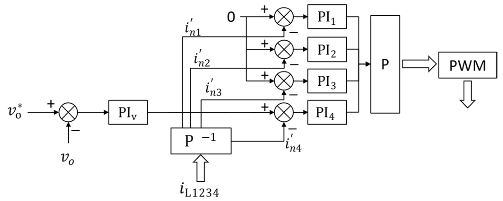
2.2. Controller
3. Power Distribution Control Strategy
3.1. Traditional Droop Control
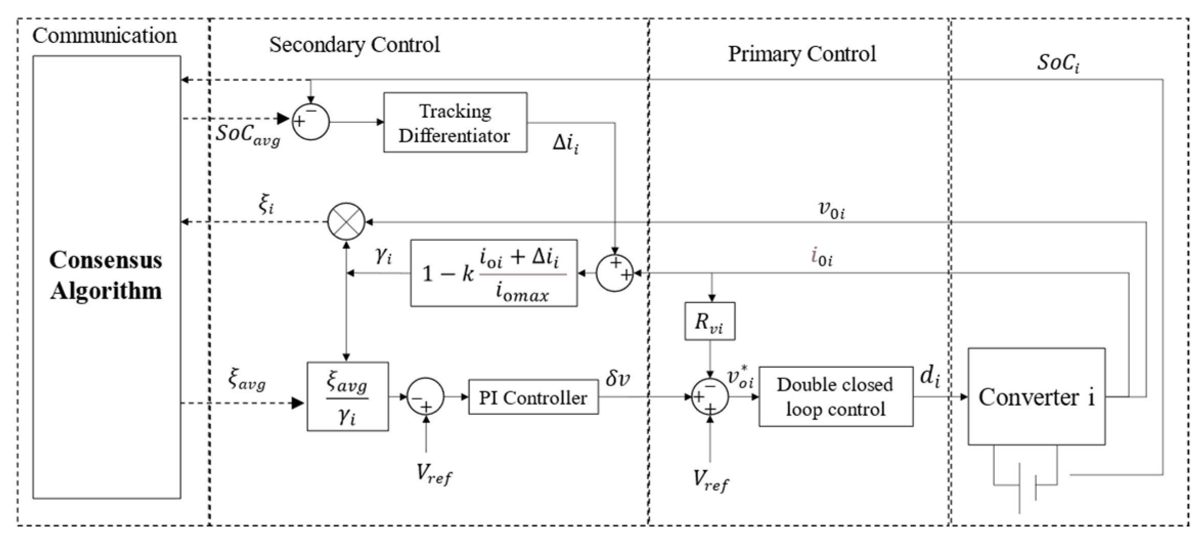
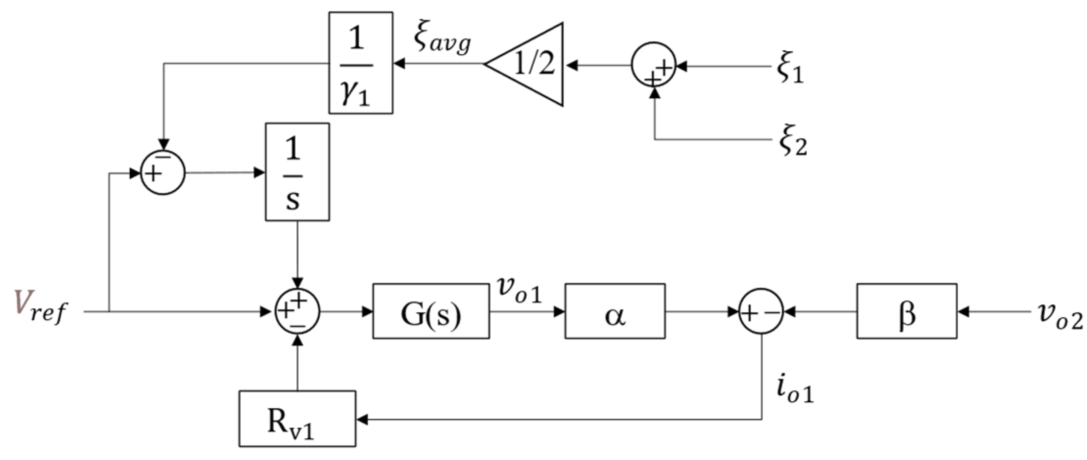
3.2. Distributed Hierarchical Control Scheme Based on Consensus Algorithm
3.3. Stability Analysis
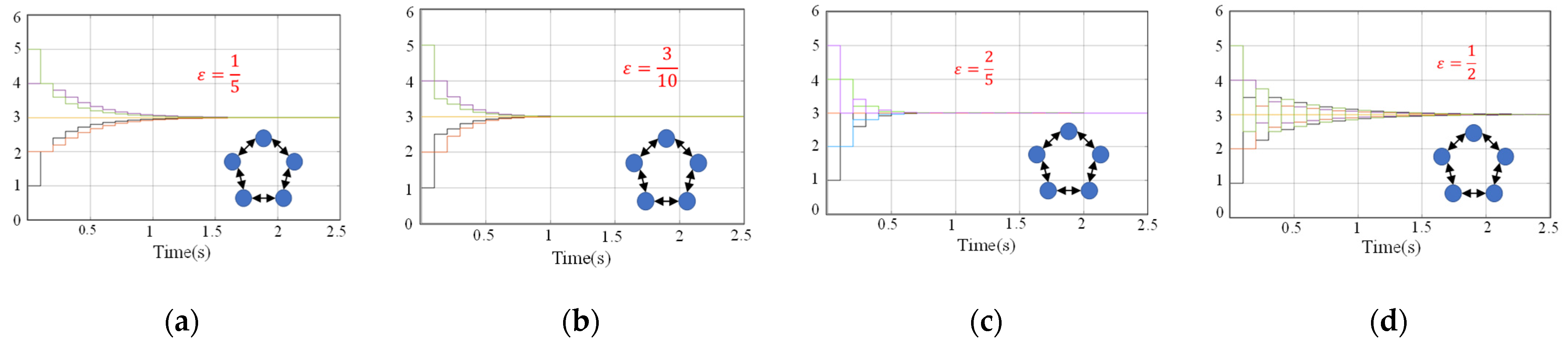
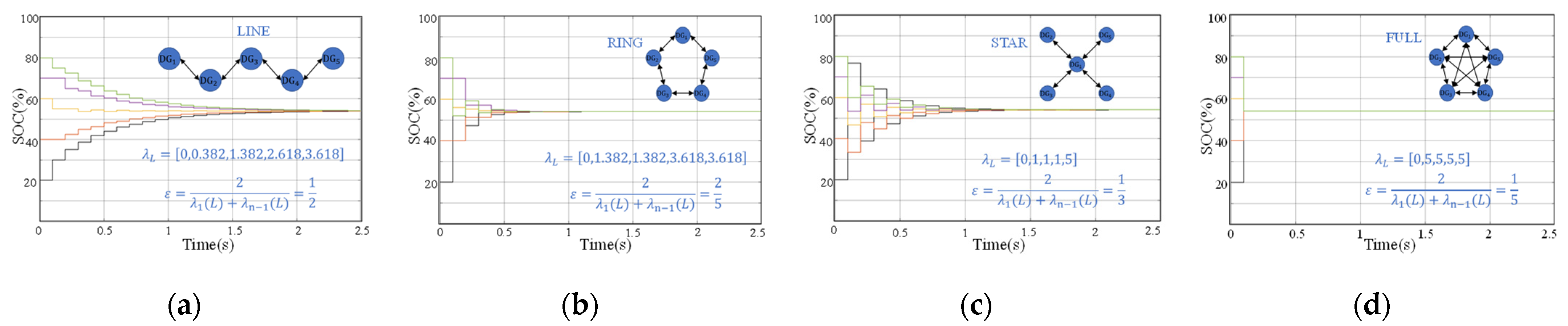
4. Consensus Algorithm
4.1. Dynamic Consensus Algorithm
4.2. Algorithm Convergence and Dynamic
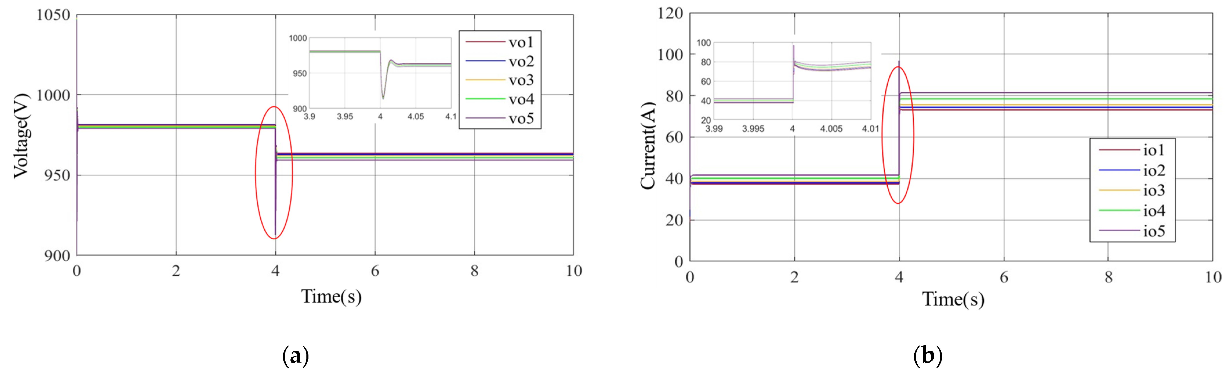
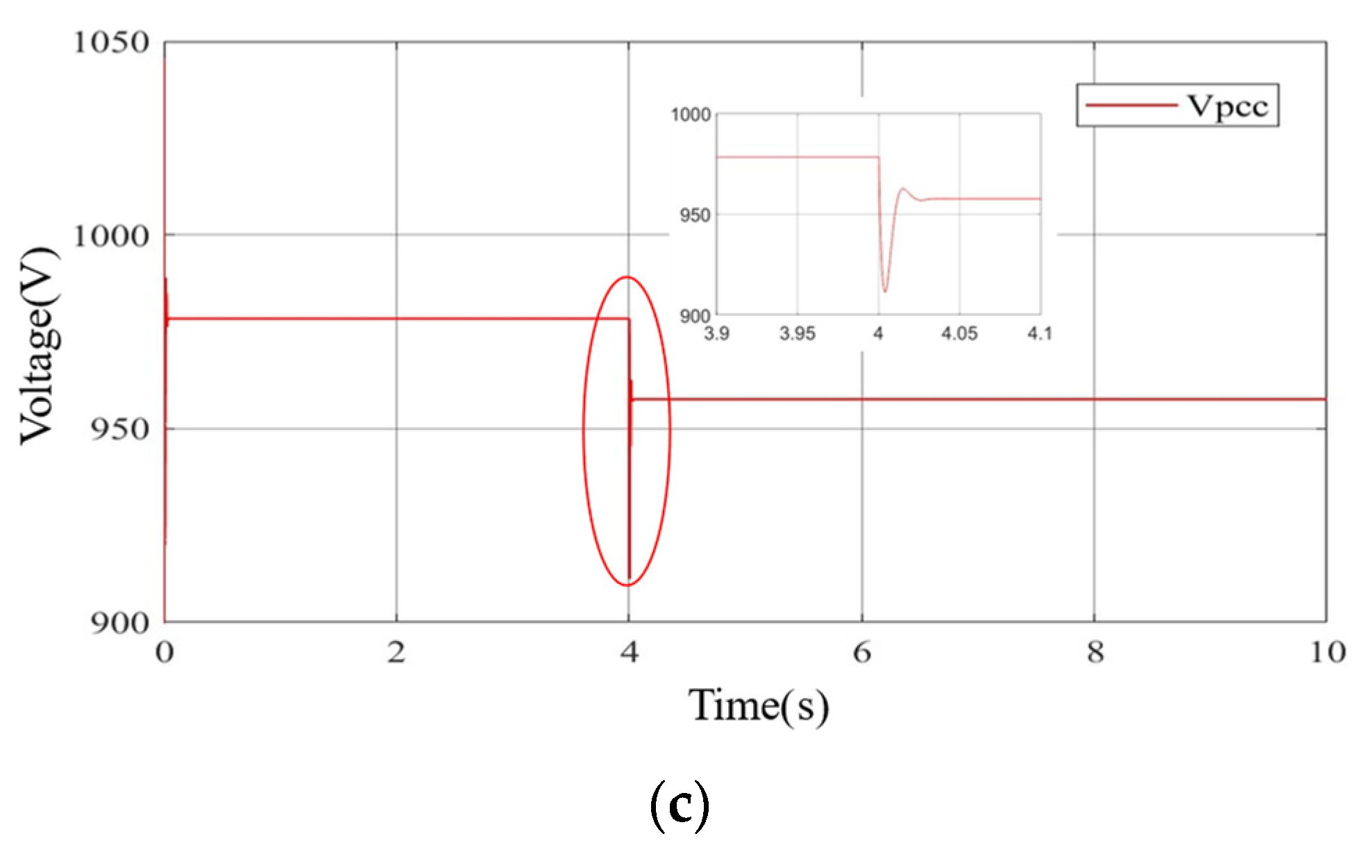
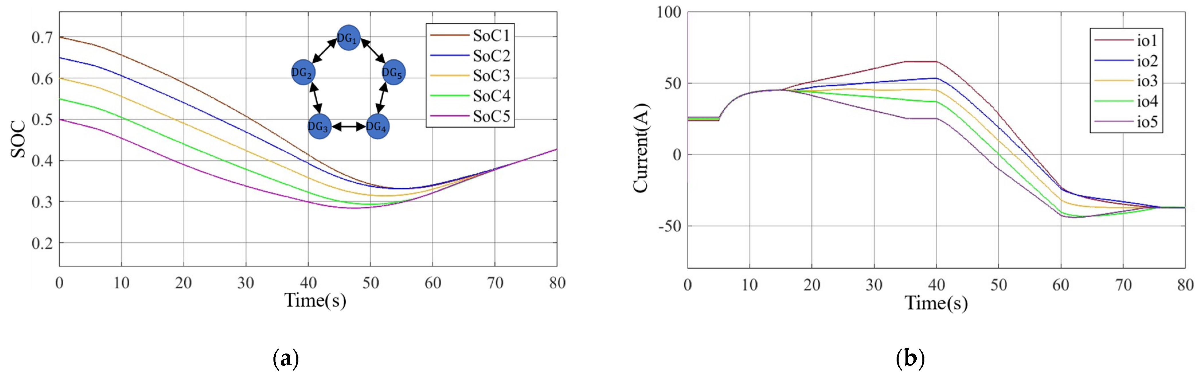
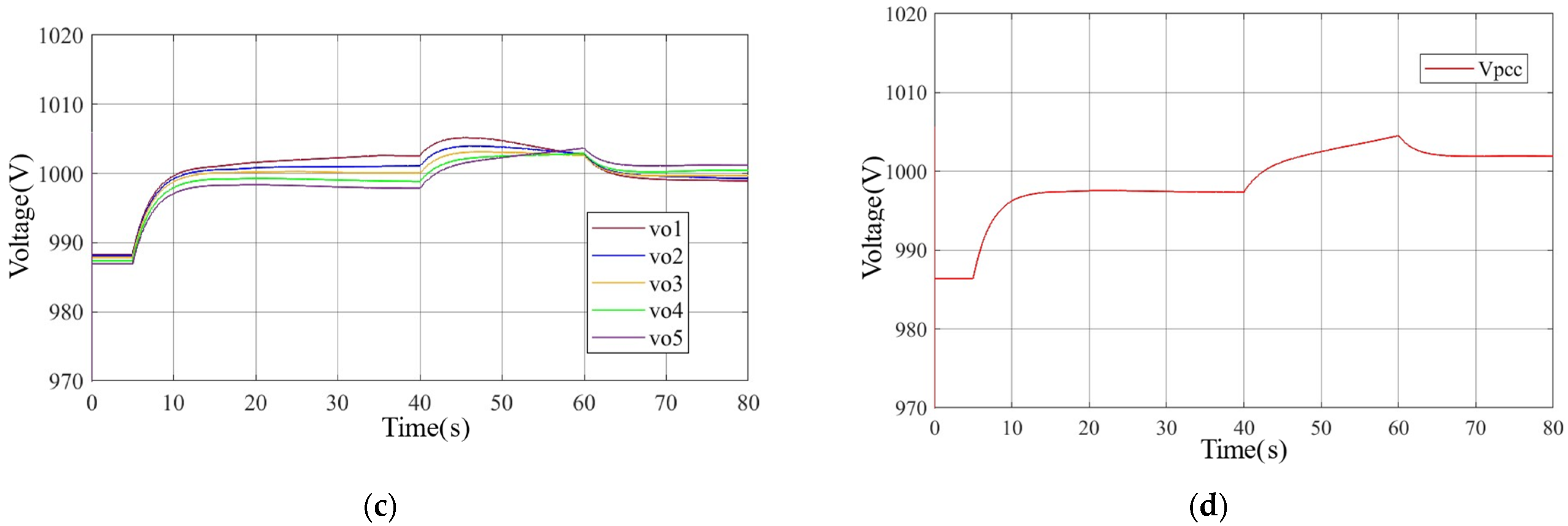
5. Simulation and Analysis
6. Conclusions
Author Contributions
Funding
Institutional Review Board Statement
Informed Consent Statement
Data Availability Statement
Conflicts of Interest
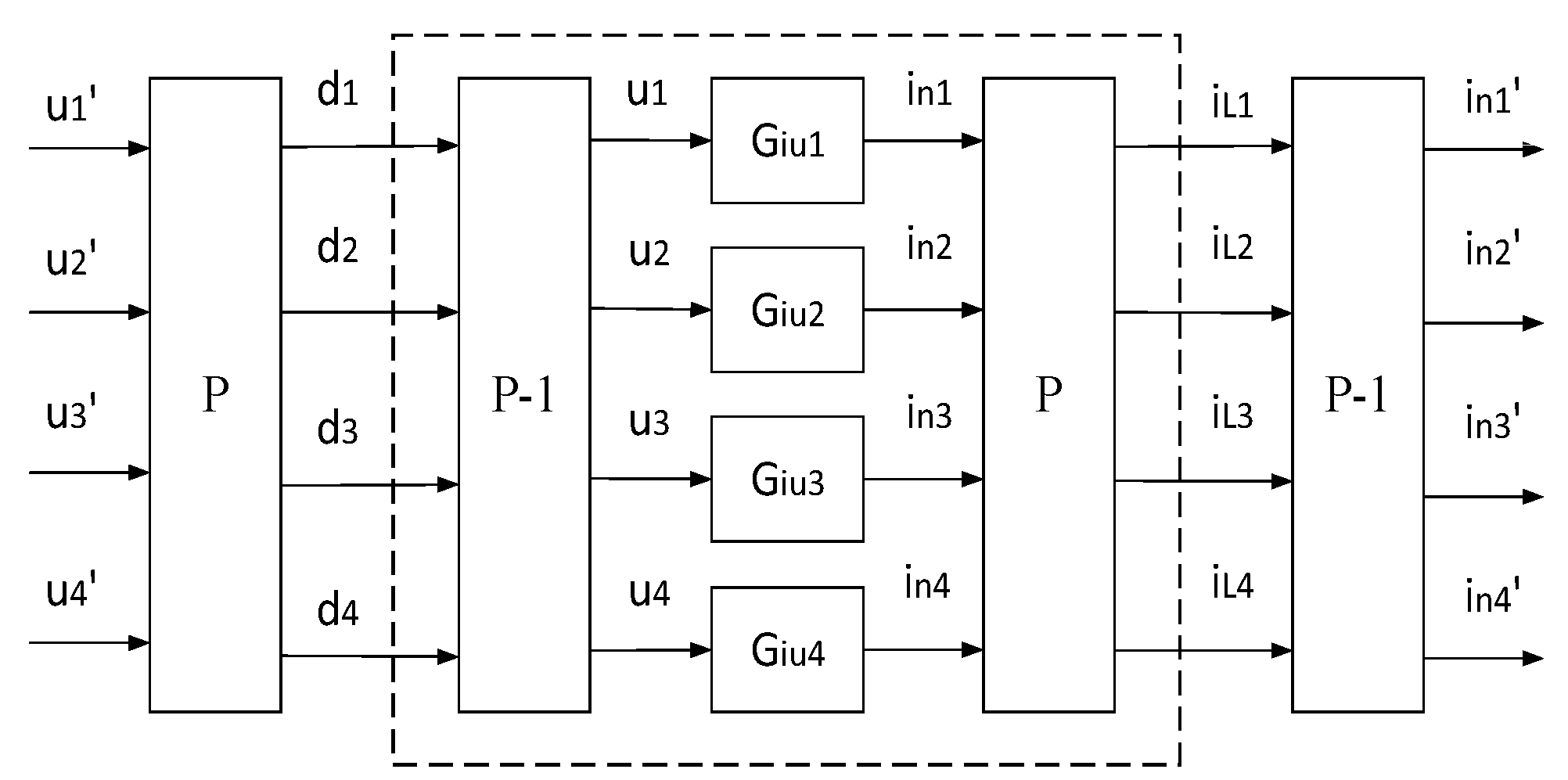
Appendix A
- (1)
- Mathematical decoupling
- (2)
- The small signal model near the steady-state is as follows:

References
- Jin, Z.; Sulligoi, G.; Cuzner, R.; Meng, L.; Vasquez, J.C.; Guerrero, J.M. Next-generation shipboard dc power system: Introduction smart grid and dc microgrid technologies into maritime electrical netowrks. IEEE Electrif. Mag. 2016, 4, 45–57. [Google Scholar] [CrossRef] [Green Version]
- Park, D.; Zadeh, M. Modeling and predictive control of shipboard hybrid DC power systems. IEEE Trans. Transp. Electrif. 2021, 7, 892–904. [Google Scholar] [CrossRef]
- Ma, Y.; Corzine, K.; Maqsood, A.; Gao, F.; Wang, K. Stability assessment of droop controlled parallel buck converters in zonal ship DC microgrid. In Proceedings of the 2019 IEEE Electric Ship Technologies Symposium (ESTS), Washington, DC, USA, 14–16 August 2019; IEEE: Piscataway, NJ, USA, 2019; pp. 268–272. [Google Scholar]
- Accetta, A.; Pucci, M. Energy management system in DC micro-grids of smart ships: Main gen-set fuel consumption minimization and fault compensation. IEEE Trans. Ind. Appl. 2019, 55, 3097–3113. [Google Scholar] [CrossRef]
- Kanellos, F.D.; Tsekouras, G.J.; Prousalidis, J. Onboard DC grid employing smart grid technology: Challenges, state of the art and future prospects. IET Electr. Syst. Transp. 2015, 5, 1–11. [Google Scholar] [CrossRef]
- Choi, C.H.; Shin, S.C.; Lee, H.J.; Jung, C.H.; Kim, H.S.; Won, C.Y. Parallel system of bidirectional DC/DC converter for improvement of transient response in DC distribution system for building applications. In Proceedings of the 2012 IEEE Vehicle Power and Propulsion Conference, Seoul, Korea, 9–12 October 2012; IEEE: Piscataway, NJ, USA, 2012. [Google Scholar]
- Nagaraja, H.N.; Kastha, D.; Petra, A. Design Principles of a Symmetrically Coupled Inductor Structure for Multiphase Synchronous Buck Converters. IEEE Trans. Ind. Electron. 2011, 58, 988–997. [Google Scholar] [CrossRef]
- Kang, T.; Gandomkar, A.; Lee, J.; Suh, Y. Design of Optimized Coupling Factor for Minimum Inductor Current Ripple in DC-DC Converter Using Multiwinding Coupled Inductor. IEEE Trans. Ind. Appl. 2021, 57, 3978–3989. [Google Scholar] [CrossRef]
- Wong, P.L.; Xu, P.; Yang, P.; Lee, F.C. Performance improvements of interleaving VRMs with coupling inductors. IEEE Trans. Power Electron. 2001, 16, 499–507. [Google Scholar] [CrossRef]
- Su, B. Research on Topology and Control of Multi-Phase Interleaved Bidirectional DC/DC Converter with Coupled Inductors. Shandong University, 2020. Available online: https://www.semanticscholar.org/paper/Multiphase-Interleaved-Bidirectional-DC%2FDC-With-for-Mayer-Kattel/6d4f88f0b5e2e29758240e92f6d3e0ea0c8bd2f3 (accessed on 10 December 2022).
- Khorsandi, A.; Ashourloo, M.; Mokhtari, H. A Decentralized Control Method for a Low-Voltage DC Microgrid. IEEE Trans. Energy Convers. 2014, 29, 793–801. [Google Scholar] [CrossRef]
- Liu, Y.; Jing, P.; Li, G. Research on the Structure and Implementations of the DC Grid Power Control. Proc. CSEE 2015, 35, 3803–3814. [Google Scholar]
- Meng, L.; Dragicevic, T.; Roldán-Pérez, J.; Vasquez, J.C.; Guerrero, J.M. Modeling and Sensitivity Study of Consensus Algorithm-Based Distributed Hierarchical Control for DC Microgrids. IEEE Trans. Smart Grid 2016, 7, 1504–1515. [Google Scholar] [CrossRef] [Green Version]
- Chen, X.; Shi, M.; Sun, H.; Li, Y.; He, H. Distributed Cooperative Control and Stability Analysis of Multiple DC Electric Springs in a DC Microgrid. IEEE Trans. Ind. Electron. 2018, 65, 5611–5622. [Google Scholar] [CrossRef]
- Liu, H. Study on Key Techniques of Stability and Coordinated Control in DC Microgrid. China University of Mining and Technology, 2019. Available online: https://www.sciencedirect.com/science/article/pii/S2352484722011210 (accessed on 10 December 2022).
- Peyghami, S.; Davari, P.; Mokhtari, H.; Loh, P.C.; Blaabjerg, F. Synchronverter-Enabled DC Power Sharing Approach for LVDC Microgrids. IEEE Trans. Power Electron. 2017, 32, 8089–8099. [Google Scholar] [CrossRef] [Green Version]
- Zhang, Q.; Chen, L.; Liu, Y.; Zhuang, X.Z.; Zheng, X.L. Power sharing control strategy based on active frequency injection in DC microgrid. Electr. Power Syst. Autom. 2021, 33, 11–19. [Google Scholar]
- Baharizadeh, M.; Golsorkhi, M.S.; Shahparasti, M.; Savaghebi, M. A Two-Layer Control Scheme Based on P–V Droop Characteristic for Accurate Power Sharing and Voltage Regulation in DC Microgrids. IEEE Trans. Smart Grid 2021, 12, 2776–2787. [Google Scholar] [CrossRef]
- Wang, W.; Zhou, M.; Jiang, H.; Chen, Z.; Wang, Q. Improved droop control based on State-of-Charge in DC microgrid. In Proceedings of the IEEE 29th International Symposium on Industrial Electronics (ISIE), Delft, The Netherlands, 17–19 June 2020. [Google Scholar]
- Micallef, A.; Apap, M.; Spiteri-Staines, C.; Guerrero, J.M.; Vasquez, J.C. Reactive Power Sharing and Voltage Harmonic Distortion Compensation of Droop Controlled Single Phase Islanded Microgrids. IEEE Trans. Smart Grid 2014, 5, 1149–1158. [Google Scholar] [CrossRef]
- Guerrero, J.M.; Vasquez, J.C.; Matas, J.; De Vicuña, L.G.; Castilla, M. Hierarchical Control of Droop-Controlled AC and DC Microgrids—A General Approach Toward Standardization. IEEE Trans. Ind. Electron. 2011, 58, 158–172. [Google Scholar] [CrossRef]
- Peng, H.; Wang, D.; Su, M. Comparative study of power droop control and current droop control in DC microgrid. In Proceedings of the 11th IET International Conference on Advances in Power System Control, Operation and Management (APSCOM 2018), Hong Kong, China, 11–15 November 2018; IET: London, UK, 2018; pp. 1–4. [Google Scholar]
- Han, J. From PID to active disturbance rejection control. IEEE Trans. Ind. Electron. 2009, 56, 900–906. [Google Scholar] [CrossRef]
- Zhang, Q.; Zeng, Y.; Liu, Y.; Zhuang, X.; Zhang, H.; Hu, W.; Guo, H. An improved distributed cooperative control strategy for multiple energy storages parallel in islanded DC microgrid. IEEE J. Emerg. Sel. Top. Power Electron. 2021, 10, 455–468. [Google Scholar] [CrossRef]
- Olfati-Saber, R.; Fax, J.A.; Murray, R.M. Consensus and Cooperation in Networked Multi-Agent Systems. Proc. IEEE 2007, 95, 215–233. [Google Scholar] [CrossRef] [Green Version]
- Olfati-Saber, R.; Murray, R.M. Consensus Problems in Networks of Agents With Switching Topology and Time-Delays. IEEE Trans. Autom. Control. 2004, 49, 1520–1533. [Google Scholar] [CrossRef] [Green Version]
- Kriegleder, M. A Correction to Algorithm A2 in “Asynchronous Distributed Averaging on Communication Networks”. IEEE/ACM Trans. Netw. 2014, 22, 2026–2027. [Google Scholar] [CrossRef]
- Biggs, N. Algebraic Graph Theory (Cambridge Tracks in Mathematics); Cambridge University Press: Cambridge, UK, 1974. [Google Scholar]
- Godsil, C.; Royle, G.F. Algebraic Graph Theory; Springer Science & Business Media: Berlin, Germany, 2001. [Google Scholar]
- Xiao, L.; Boyd, S. Fast linear iterations for distributed averaging. Syst. Control Lett. 2004, 53, 65–78. [Google Scholar] [CrossRef]
- Xu, L.; Guerrero, J.M.; Lashab, A.; Wei, B.; Bazmohammadi, N.; Vasquez, J.C.; Abusorrah, A. A Review of DC Shipboard Microgrids Part II: Control Architectures, Stability Analysis and Protection Schemes. IEEE Trans. Power Electron. 2021, 37, 4105–4120. [Google Scholar] [CrossRef]


| Device Parameters/Units | Value | Control Parameters/Units | Value |
|---|---|---|---|
| Inductance L/mH | 2.5 | TD Adjustment coefficient h0 | 1 × |
| Mutual inductance M/mH | −2 | TD filter coefficient r0 | 1 × 10³ |
| Output capacitance C2/μF | 1000 | Secondary control kp | 0 |
| Battery voltage v1/V | 500 | Secondary control ki | 1 |
| Battery capacity Sn/kwh | 2 | Communication latency Tca/ms | 100 |
| Maximum output current of converter /A | 100 | Bus Voltage/V | 1000 ± 10% |
Publisher’s Note: MDPI stays neutral with regard to jurisdictional claims in published maps and institutional affiliations. |
© 2022 by the authors. Licensee MDPI, Basel, Switzerland. This article is an open access article distributed under the terms and conditions of the Creative Commons Attribution (CC BY) license (https://creativecommons.org/licenses/by/4.0/).
Share and Cite
Zeng, H.; Zhao, Y.; Wang, X.; He, T.; Zhang, J. Modeling of Ship DC Power Grid and Research on Secondary Control Strategy. J. Mar. Sci. Eng. 2022, 10, 2037. https://doi.org/10.3390/jmse10122037
Zeng H, Zhao Y, Wang X, He T, Zhang J. Modeling of Ship DC Power Grid and Research on Secondary Control Strategy. Journal of Marine Science and Engineering. 2022; 10(12):2037. https://doi.org/10.3390/jmse10122037
Chicago/Turabian StyleZeng, Hong, Yuanhao Zhao, Xuming Wang, Taishan He, and Jundong Zhang. 2022. "Modeling of Ship DC Power Grid and Research on Secondary Control Strategy" Journal of Marine Science and Engineering 10, no. 12: 2037. https://doi.org/10.3390/jmse10122037