On the Development of a Mid-Depth Lagrangian Float for Littoral Deployment

Abstract

This study presents the complete, detailed development process of an enhanced one-man portable Lagrangian float designed for littoral deployment to depths of up to 300 m. The design focused on maximization of the Lagrangian characteristics of the hull, minimization of the noise emission and energy efficiency of the propulsion system, and the versatility of the platform for various scientific missions. The platform is propelled by a variable buoyancy engine that is actuated by an oil-submerged, gas-pressure assisted micro gear pump. The pressure assistance lowers the pressure differential across the pump ports at depth, resulting in quieter and more efficient operation. An enhanced proportional–integral–differential control scheme is employed to pilot the platform. To enhance diving safety, a software safety agent was incorporated. If the software safety agent detects a major failure, a drop weight is released. To eliminate the chance of water ingress through dynamic hull penetration, the drop weight is actuated by an in-house developed magnetic coupling mechanism. An onboard installed hydrophone continuously records and monitors ambient sounds for phenomena of interest and enables commands and mission updates from the surface. For surface recovery, the platform is equipped with GPS and an Iridium beacon for long-range localization, and an RF beacon and strobe for short-range localization and as a backup. The performance of the platform is demonstrated in a simulation and in an actual real sea mission conducted in the eastern Mediterranean at a depth of 10 and 12 m.

1. Introduction

Lagrangian floats (LF) have been employed in ocean exploration since the 1950s [1,2]. Initially, floats had no active buoyancy control and had to be precisely ballasted for a specific desired depth. To rise to the surface, a float would drop a designated weight, either following an acoustic command or on a timed trigger, and resubmerging required human intervention. The first LF with active buoyancy control were the autonomous Lagrangian circulation explorers (ALACE), developed in the 1980s, with first prototypes deployed in 1988 [1,2,3]. These floats transferred hydraulic fluid between an internal reservoir and an external bladder in order to adjust the float’s density, and so were capable of resubmerging multiple times to a range of depths rather than to a single predefined depth.

Generally, LF are equipped with active propulsion only in the vertical (heave) direction, and usually such propulsion systems consist of a variable buoyancy engine (VBE). A VBE operates by adjusting the density of the float to match the water density at a desired depth, thus bringing the float to neutral buoyancy at that depth. This is achieved by changing either the float’s mass or volume while maintaining the other property constant. Changing float mass is usually achieved by ingestion (expulsion) of ambient water into (out of) an internal compartment of the float [4,5]. A less common method is equipping the float with extra ballast apportioned into multiple small parcels, such as bearing balls, and expelling them in a controlled manner during the mission [6]. Changing float volume is usually achieved either by inflating (deflating) an external elastomeric bladder [3,7,8] by transferring liquid from (/into) a reservoir inside the float, or by extending a rigid piston from the float [9,10,11] or a section of the float itself [12]. These methods are generally actuated by either a reciprocating pump [3,8] or a motor and lead screw system [4,7,11,13].

The largest and most well-known scientific study employing LF and profiling floats is the international Argo program, https://argo.ucsd.edu/, accessed on 17 December 2022. Currently, this program consists of more than 4000 floats having different configurations, performing 10-day long profiling cycles from the ocean surface to depths between 2000 and 6000 m [1,8]. Gathered data are transmitted to onshore data centers via satellite and freely accessible to the public via the internet, usually within 12 h. Floats developed for the ARGO project have also been used in the study of internal waves (IW) [14,15].

Traditionally, LF have been deployed in the open ocean, reaching great depths; they generally kept away from shallow waters and the seafloor. In recent years, there has been increased interest in LF as platforms for exploration of littoral waters due to their relatively low cost, energy efficiency and ease of deployment. The increased interest from the local scientific community together with the lack of IW data for the eastern Mediterranean Sea (EMS) called for the development of this mid-depth Lagrangian float (MDLF).

In recent works, shallow to mid-depth LF were developed for different mission types: profiling [10], study of underwater currents and IW [12], constant altitude [4] (contour following) photographic surveys of the seabed [11] and of scattering layers [7]. Usually, the design of each float was biased towards its planned mission type by adding or omitting certain design aspects.

On the size scale of such floats, the horizontal displacement of water is predominantly governed by pressure differences rather than viscosity [9]. Thus, the movement of a body with density exactly equal to that of the surrounding water, therefore having the same linear inertia, will be driven by the same pressure gradients, and the body will move as one with the water in the horizontal plane. Consequently, only vertical motion is considered in our LF design and in the development of the equation of motion and dynamic model.

Generally, compressibility matching between the float and water has a major impact on the Lagrangian behavior of the former [16]. When float and water compressibilities differ, and the water moves vertically due to some disturbance, e.g., IW, the resulting pressure change will affect water and float to a different degree. Consequently, the float may not faithfully follow the vertical movement of the water [17]. Nevertheless, since in shallow waters and upper water layers, water temperature and salinity have a much stronger effect on water density than pressure and vertical water movements are relatively small, the effect of compressibility on the float’s Lagrangian behavior is limited. As a result, to simplify the design and eliminate additional dedicated components (i.e., “compressee” [18,19]) when designing shallow depth floats, compressibility matching of the float’s hull was frequently waived [4,12]. For the enhanced float developed here, compressibility matching was inherently achieved through a careful design of its hull without the need to add any additional external dedicated component.

Contour following floats require an altimeter to maintain a constant distance from the seafloor. In addition, they need a more accurate and faster depth control mechanism compared to other LF. Such floats may also benefit from the addition of thrusters [20] to a VBE for maintaining an accurate altitude from the seabed as required for photographic surveys and stereophotography in particular. As the float developed here is intended to operate in shallow to mid-depth littoral waters and possibly close to the seabed, an altimeter was integrated to prevent collision with the seabed. This altimeter could also be employed in an altitude-maintaining control loop if required.

Usually, LF are pressurized vessels that maintains their internal pressure at an approximately constant atmospheric. This means that a typical VBE experiences a zero-pressure differential while on the sea surface and greatest pressure differential at maximum deployment depth. Pressure assistance or pre-tensioning of the VBE reverses the pressure levels experienced by the VBE. A pressure assisted VBE is under increased pressure differential on the sea surface and a decreased pressure differential at depth. Consequently, a strictly profiling float will experience only an inversion of the pressure differential across the VBE, resulting in little benefit. In contrast, for a float that spends most of its mission at depth, pre-tensioning of the VBE will result in a reduced pressure differential during most of its mission and actuation time of the VBE, thus resulting in a decrease in power consumption [5]. In addition, a passively pre-tensioned buoyancy engine may serve as a failsafe surfacing mechanism [5]. Furthermore, this pre-tensioned or pressure assisted design extends the feasibility of using a VBE driven float for contour following missions to much greater depths compared to a regular VBE, possibly eliminating depth as a limiting factor for VBEs as actuators in contour following missions.

Strictly profiling floats may forgo Lagrangian design considerations. Floats that employ acoustic scientific equipment for positioning, communication or recording of ambient sounds require a silent means of propulsion to minimize emitted noise and consequent interference with the onboard acoustic equipment. Due to the variety of missions anticipated, Lagrangian characteristics and a quiet propulsion system were set as key requirements in the design of the float developed in this work.

The MDLF in this study was designed as a low-cost Lagrangian platform for littoral deployment to depths of up to 300 m for a variety of scientific missions.

Table 1. Float main physical parameters.

Parameter	Value
Internal hull diameter	150 mm
External hull diameter including stiffeners	180 mm
Hull length	858 mm
Overall length, including endcap instruments	1360 mm
Hull weight	7600 g
Fully equipped, non-ballasted float weight	19,450 g
Fully equipped, non-ballasted float volume	19,730 cc

presents the main physical parameters of the developed float.

The MDLF’s propulsion system is based on a VBE equipped with a relatively large bladder capacity of >3% of the overall float volume, compared to 1.85% for 100 m depth in [8], 0.2% for 2000m and 1.5% for 250 m in [9]. This large bladder provides the MDLF a high positive buoyancy reserve that permits an increased upward heave speed and, upon surfacing, allows exposure of the antenna enclosure for reliable satellite communication. To maximize Lagrangian behavior, the float’s hull was carefully designed with a compressibility close to the average compressibility of the local water column. The compressibility matching was implemented into the design of the main pressure hull instead of using an external compressee [18,19], thus eliminating the need for an additional external component. A submerged, gas-pressure assisted micro gear pump actuates the VBE. This configuration reduces the pressure differential on the VBE at depth, allowing for a quieter and more efficient operation. In addition, the gas pressure assistance allows the easy adjustment of the pre-tensioning of the VBE pressure to the expected average mission pressure requirement for optimal performance. The float is equipped with four pressure and four temperature sensors, two at each endcap [19]. This configuration allows redundancy and a lower measurement error as well as the ability to calculate values at the geometric center of the float. An onboard hydrophone continually records ambient sounds and allows the float to receive commands from the surface. A magnetically coupled emergency drop-weight, controlled by a dedicated and isolated controller and battery, enables, in case of a major failure, emergency surfacing. Upon surfacing, a GPS/Iridium beacon enables long-range localization while an RF beacon serves as backup.

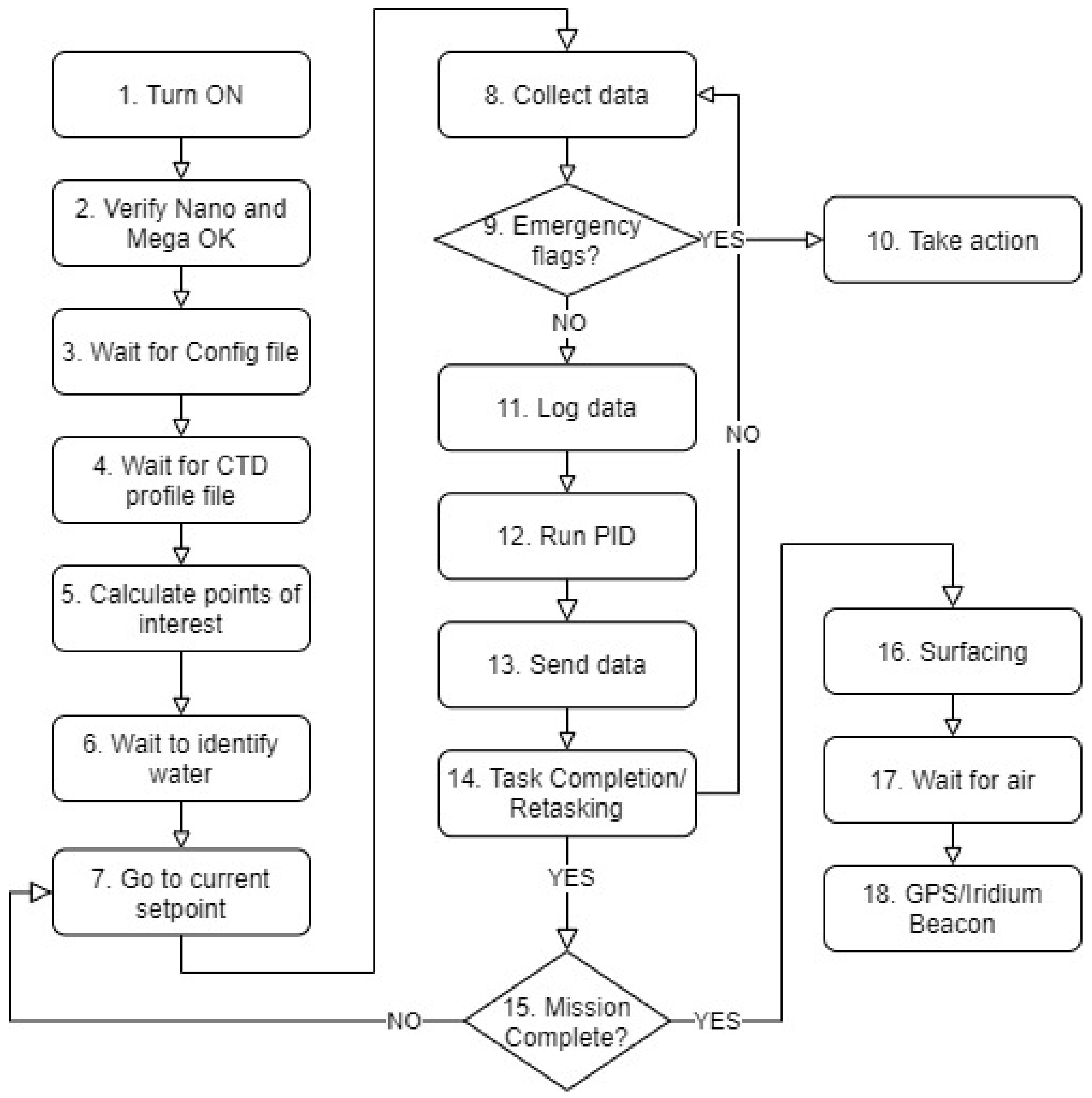
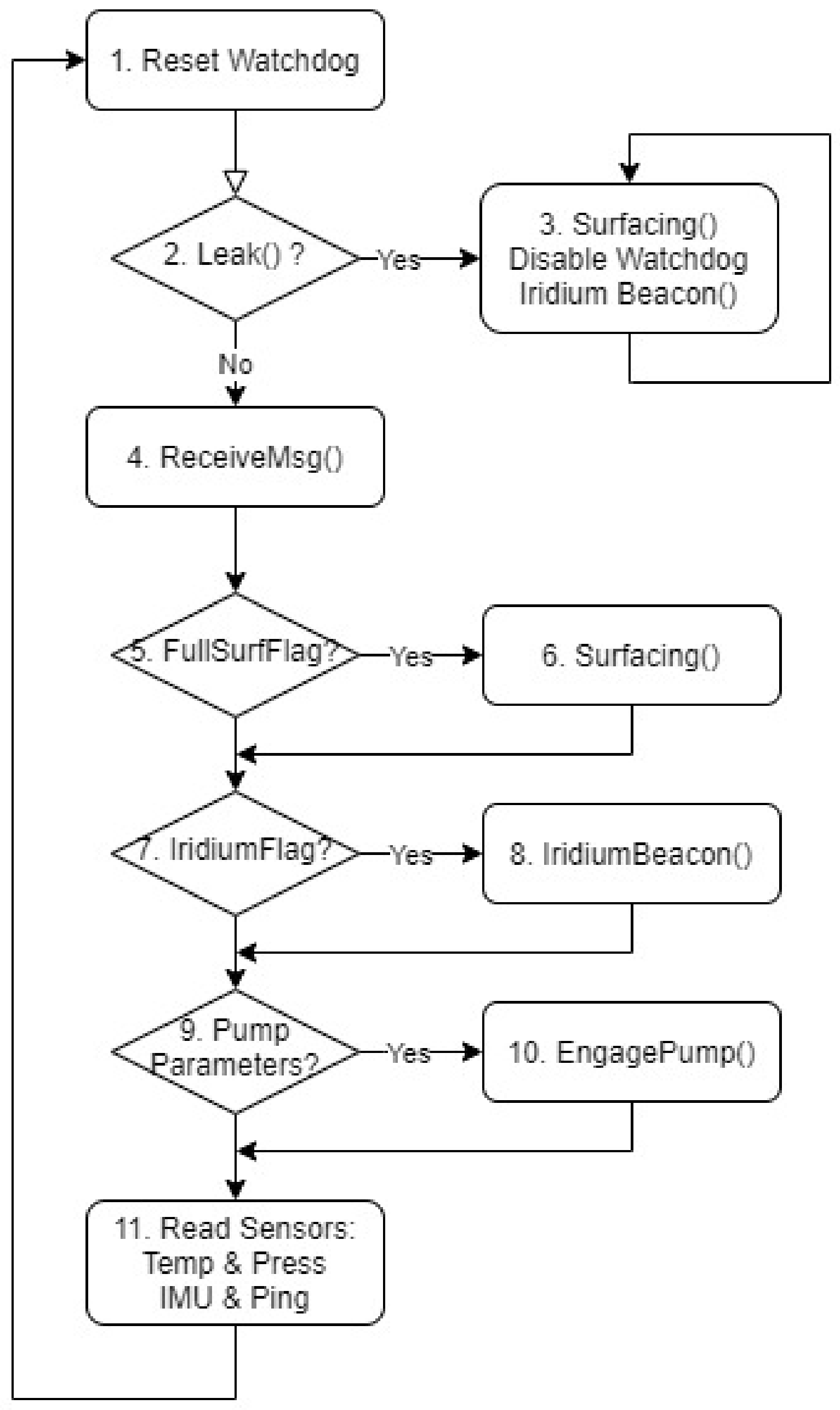
The paper is organized as follows: In Section 2, the float design process is presented. A description of the equation of motion, the developed dynamic model and the development of the controller for the propulsion system is provided in Section 3. Section 4 briefly describes the float software architecture. Section 5 contains the testing procedures and alpha trial experimental results. Discussion and concluding remarks are presented in Section 6.

2. Design Process

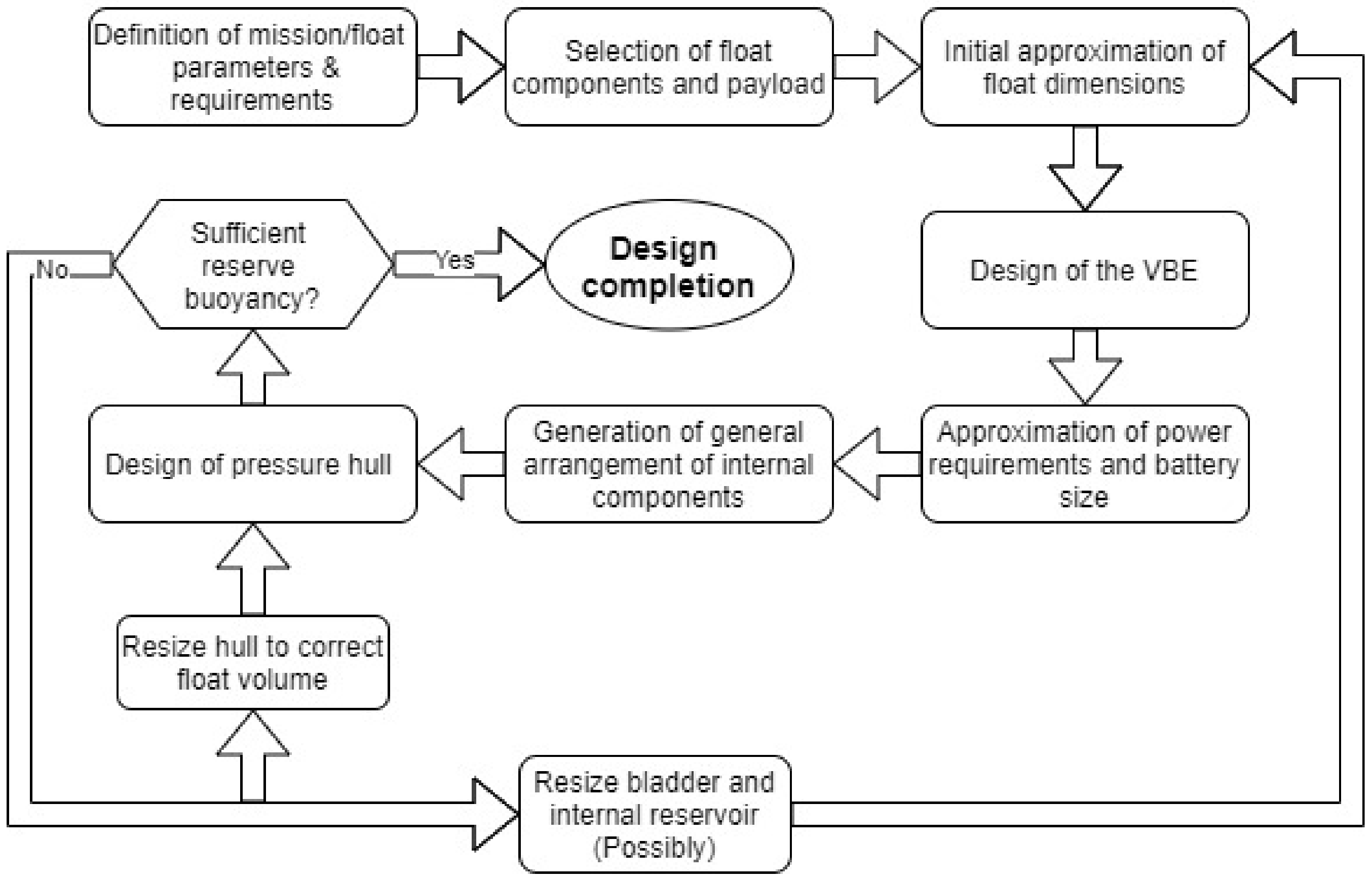
The goal of this work was to develop and construct a float that can serve as a multipurpose platform for various scientific missions with IW as the reference mission. Therefore, it was decided to equip the float with a payload and capabilities that will allow it to fulfill both profiling and Lagrangian missions. These objectives meant that the float should be capable of (1) profiling, (2) isobaric (depth/pressure keeping) and (3) isopycnal (density keeping) modes, as well as normal or emergency surfacing and reliable localization following surfacing. Moreover, the float shall have a reserve of internal space and buoyancy to accommodate additional future payload and electronics. This study focused on the platform engineering development through all its aspects with the main design stages summarized in the form of a design spiral shown in Figure 1 and described below.

2.1. Mission Parameters and Float Characteristics

The initial mission requirements and parameters were defined in collaboration with our partner oceanographers. As almost no data is available on IWs for the EMS area, IW were defined as the main phenomena of interest and primary mission. The maximum operating depth was set to the depth of the Israeli shelf break of 300 m since it was concluded that local IWs would be predominant in this depth range. Maximum mission duration was set to 24 h.

Based on the above mission parameters, the required float characteristics were defined as:

• A pressure hull rating of 300 dbar;
• Equipped with platform sensors: pressure, temperature and IMU;
• Equipped with a hydrophone to record ambient sounds, specifically the sound of breaking IWs (if such exist), localization and reception of acoustic commands from surface platforms, e.g., the mission support boat.

In addition, based on previous studies available in the literature, some additional platform related requirements were defined:

• Maximization of the Lagrangian float characteristics by matching hull compressibility to the average compressibility of the local water column;
• Low-noise propulsion to avoid interference with onboard acoustics.

Lastly, a set of additional requirements that were deemed appropriate for coastal missions were added.

• One-man-portable and deployable from a small support boat to lower costs of utilization and allow for quicker and more flexible deployments;
• Lower cost by utilizing off-the-shelf components to the maximum possible extent;
• Reduce chances of float loss by addition of dedicated safety hardware and software.

Based on the above listed requirements, specific float components and payload were selected. The main float components are listed in

Table 2. Main float components.

System	Component	Component Data
VBE	Pump	MG2000S by TCS Micropumps Ltd.
	Valve	SV08 spool valve & 24 V solenoid by HydraForce Inc.
	Bladder	0.7 L by EPE ITALIANA S.r.l.
Sensors	Pressure Sensor	Bar30 by Blue Robotics Inc.
	Temperature Sensor	Celsius Fast-Response by Blue Robotics Inc.
	IMU	Qwiic VR IMU by SparkFun Electronics
	Altimeter	Ping Sonar by Blue Robotics Inc.
Comms/Beacons	GPS Module	XA1110 (Qwiic) by SparkFun Electronics
	Iridium Module	RockBLOCK 9603 by Rock Seven Mobile Services Ltd.
	Iridium Antenna	M1621HCT-P-SMA by Maxtena Inc.
	RF Beacon	RF-700C1 by Metocean Telematics
Controllers	Main controller	Raspberry Pi 3 Model B
	I/O controller	Arduino Mega
	DW controller	Arduino Nano
DW Mechanism	DW gear-motor	6 VDC, 31 RMP, 12 kg/cm, 12 g
	DW motor driver	MAX14870 brushed DC motor driver by Pololu
Batteries	Main battery	22.2 V/17.25 Ah Li-Ion by Amicell Ltd.
	Controllers’ battery	7.4 V/3.7 Ah Li-Ion
	Drop-weight battery	7.4 V/1 Ah Li-Ion
Misc.	Leak detector	SOS Leak Sensor by Blue Robotics Inc.

.

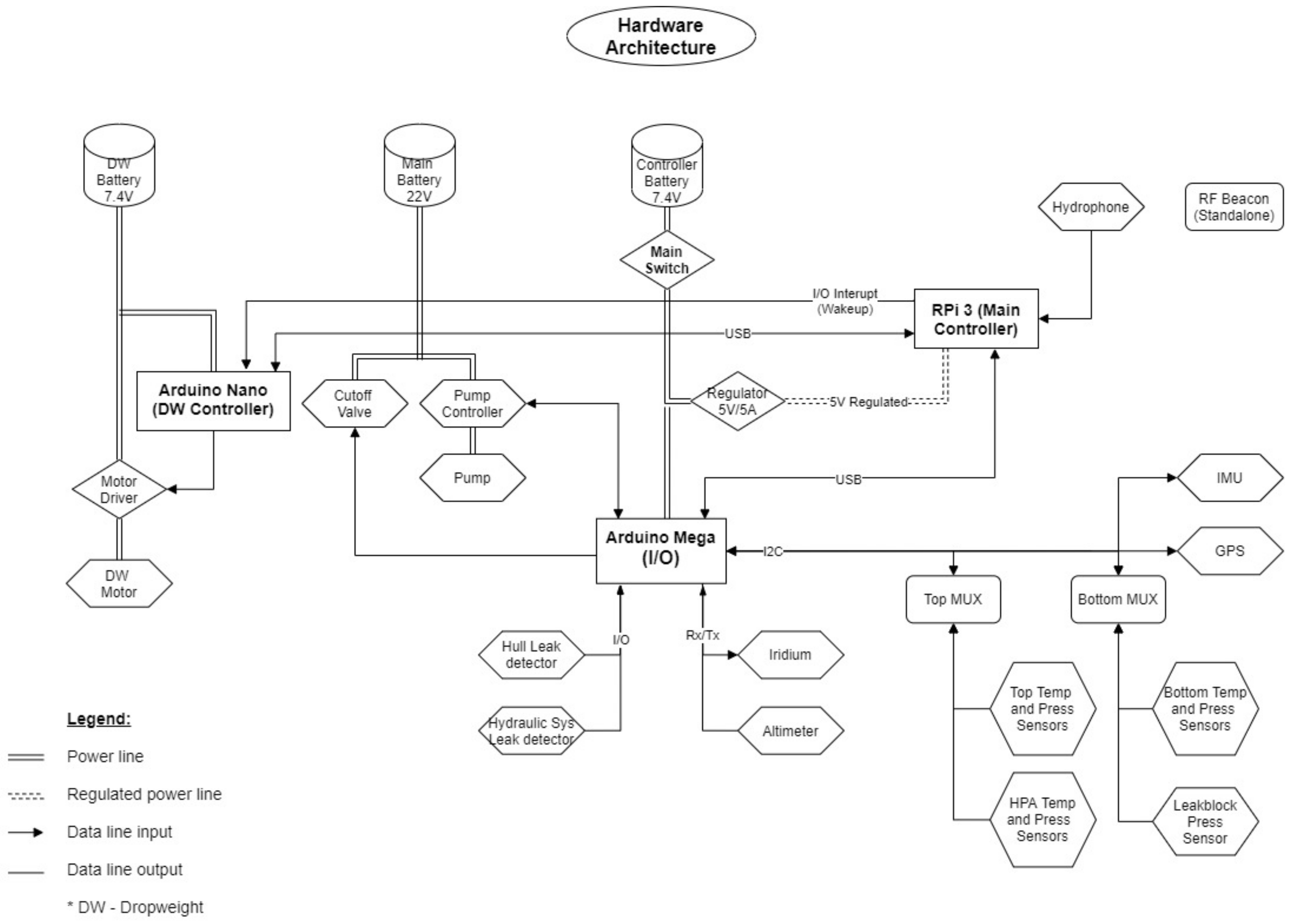
The complete float hardware architecture is presented in Figure 2, including the three controllers, batteries and sensors. A RaspberryPi 3B serves as the main controller and is connected to the two secondary controllers (Arduino based) via USB and to the onboard hydrophone. All the platform sensors are connected to the Arduino Mega (I/O controller) via an I2C bus through two multiplexers. The sensors on each endcap are assigned to a specific multiplexer. An Arduino Nano powered by a dedicated power supply serves as the DW controller.

The description of the platform’s components follows the design process where the sensors, scientific payload and hardware were the first to be selected and designed, followed by the development and design of the propulsion system and, lastly, the hull.

2.2. Sensors

For navigation and motion control, the float is equipped with four temperature and four pressure sensors, with two per endcap. This geometrical division allows us to calculate the pressure and temperature values at the float’s geometrical (buoyancy) longitudinal center. In addition, the extra number of sensors provides redundancy in case of sensor failure and lowers measurement errors. Expression for the standard error is presented in Equation (1):

$$SE=\frac{\sigma }{\sqrt{N}}$$

(1)

where $SE$ is the standard error, $\sigma$ is the sensor error and $N$ is the accumulated number of averaged measurements. The error is decreased further by using a 5-point moving average for each sensor, possible due to the sensors’ fast response—approximately 50 ms for each—compared with the relatively slow time constant of the float motion. Two sensors with five measurements each result in $N=10$ and consequently a reduction of the measurement error by $\sqrt{10}=3.16$. The error of the temperature and pressure sensors is $\pm 0.1 ℃$ and $\pm 200 \mathrm{mbar},$ respectively, and after averaging the resulting measurement, error is decreased to $\pm 0.032 ℃$ and $\pm 63 \mathrm{mbar}$, respectively.

An altimeter with a range of 30 m is installed at the bottom of the float. It is currently dedicated to collision avoidance with the seafloor only but may be employed in the future in a terrain following operational mode. Low frequency cyclic fluctuation in water density and temperature may indicate the presence of IW. Monitoring the external pressure and the heave acceleration for such cyclic fluctuations while maintaining constant density, which in the absence of vertical forcing should translate to constant depth of the float, is one mechanism of detecting IW. Consequently, an IMU is installed as an additional navigation sensor and is currently employed in measuring heave acceleration to identify, in post-processing, and in conjunction with the pressure sensors, vertical motion and, specifically, IW induced motion. Alternatively, maintaining constant depth while monitoring temperature fluctuations is another IW detection method.

In view of the float’s relatively short mission duration and the corresponding short roaming range, it was concluded that salinity changes over the duration of the mission may be neglected. Therefore, it was decided that a salinity sensor would not be installed onboard (also because of its high cost and operation complexity). Prior to float deployment, a small CTD would be deployed, and the salinity profile of the CTD would be uploaded to the float and serve as a look-up table during the mission.

The non-navigational platform’s sensors include a leak sensor that is attached to the bottom endcap and a second one embedded in the hydraulic tubing to detect ingress of water in case of bladder failure. Additional sensors are an integral part of the VBE and are described in the VBE section.

The platform’s dedicated sensors also include an M36-900 hydrophone manufactured by GeoSpectrum Technologies Inc. (Darthmouth, NS, Canada). The hydrophone continuously records and monitors ambient sounds for phenomena of interest and for acoustic commands. When a phenomenon of interest or acoustic command is detected, the float’s current mission may be halted by the acoustic module and an interrupt mission will be defined by the controller. Once the interrupt mission is completed, based on a time constraint, the float resumes its original mission.

2.3. Controllers

The float is equipped with three controllers with a RaspberryPi 3B (Pi) as the main controller which handles data logging and most computations, including the navigation proportional–integral–differential (PID) controller and acoustic data analysis. The secondary controller is an Arduino Mega (Mega), which handles most of the I/O, including sensors and pump control. The third is an Arduino Nano (Nano), which serves as a standalone controller for the DW system. To enhance its survivability in case of a major failure it is housed in a separate enclosure with a dedicated power supply and the DW mechanism.

2.4. Communications and Beacons

For communication, localization and post mission recovery, the float is equipped with several instruments. For underwater localization, a standalone miniature acoustic pinger is installed, which allows surface platforms to follow the float’s position. For post-mission long-range surface localization, the float is equipped with GPS and Iridium modules. Both modules are housed in a dedicated external enclosure connected to the Mega via watertight penetrations for both power and control. To avoid substantial signal losses associated with connecting SMA cables, it was decided to install the GPS and Iridium modules in the external enclosure rather than using external antennas. For post-mission short-range (up to 5 km) surface localization and as a backup, the float is equipped with a standalone HRF beacon and strobe combo. The RF beacon is completely independent of the float systems. It is turned on at mission start and has up to eight days of continuous operation time using its internal batteries.

2.5. Drop-Weight (DW) Mechanism

To prevent the loss of the float due to a major system failure, an emergency surfacing capability was considered essential; consequently, a DW system was developed and integrated. The DW mechanism is housed in a separate enclosure installed at the bottom end of the float, as presented in Figure 3. The DW mechanism was designed in-house with the goal of maximizing its independency and robustness. To that end, the mechanism is self-contained with its own controller, battery, motor and motor controller, and is realized without any dynamic seals. The design is based on the concept of magnetic coupling and includes a ring-shaped, 750 g steel drop-weight supported by a spoke-wheel bracket. The DW controller, Arduino nano, draws approximately 0.2 W through the entire mission duration. The DW motor will draw 0.6 W for 20 s if the DW has to be released.

A pin with an embedded permanent magnet (magnetic pin) is fixed to the center of the supporting bracket and magnetically coupled to a permanent magnet installed on the internal side of the enclosure. The internal magnet is embedded into a threaded bronze slider driven by a lead screw connected to a miniature motor. In the DW “hold” position, both magnets are aligned; when a release command is received, the motor turns and the internal magnet travels along the lead screw. Once the two magnets are misaligned, the magnetic connection is lost and the drop-weight is released. A cable connects the main controller to the DW controller with a heartbeat protocol running on both controllers. Each controller executes a cyclic 20 s resetting timer, unless a signal (heartbeat) is received from the other controller in the allotted time the controller performs a preset emergency response. If the signal is received in the allotted time the timer is reset and the cycle is repeated. Should the main controller become nonresponsive, or an emergency ascent command be received, the DW controller drops the DW. Alternatively, if the DW controller is nonresponsive, the main controller initiates a mission abort.

2.6. Variable Buoyancy Engine (VBE)

As part of the design phase, several alternatives for the VBE configuration were considered. Coastal waters may be highly turbid and, in the EMS, usually have high salt content. Hard particulates such as sand and salt can easily damage the seals of a sliding plunger. Hence, it was decided to employ a closed bladder and internal reservoir system rather than an open system, i.e., one reliant on ingestion of ambient water or an extending piston. To comply with our goal of using off-the-shelf components, it was decided to use a commercial miniature pump; accordingly, the VBE design commenced with the search for a miniature, high-pressure, low-noise and moderate cost pump.

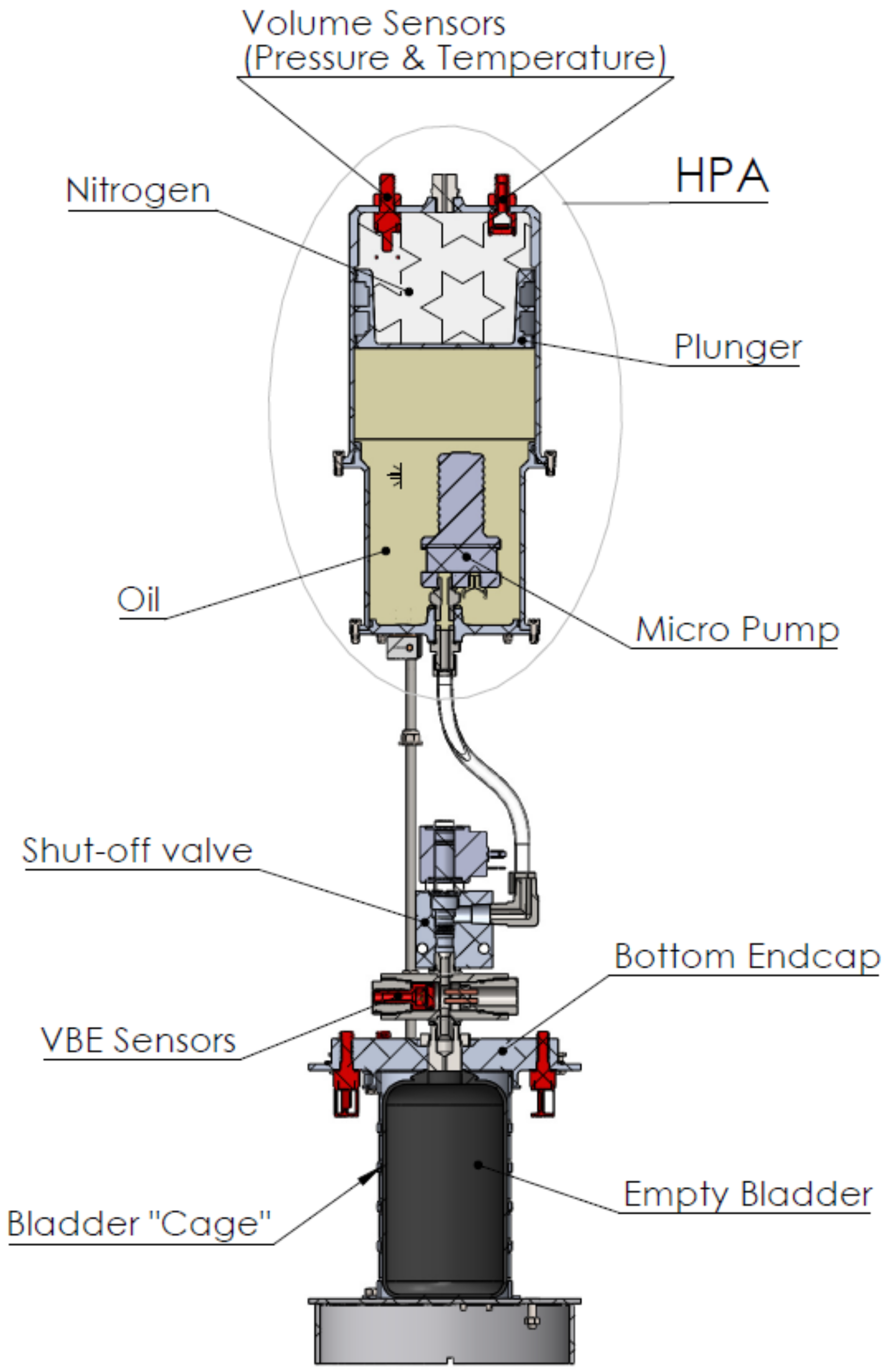
To optimize the VBE performance at the characteristic mission depth (power consumption and emitted noise), it was decided to submerge the pump within the VBE fluid and pressurize the fluid. A dedicated hydropneumatic accumulator (HPA) was designed for this purpose. The VBE design is presented in Figure 4. In the HPA, pressurized nitrogen is separated from the ballasting fluid (transformer oil) by a free-moving plunger. The pump, submerged in the ballasting fluid, transfers the fluid from the HPA through a tube, shut-off valve and sensor block into the bladder. The plunger movement is physically limited at both the “bladder full” and “bladder empty” positions. For a maximum depth deployment (300 m) the nitrogen pressure fluctuates between 10 and 20 barg depending on the momentary bladder volume; accordingly, the nitrogen would be filled to a lower pressure for a shallower deployment so that the pressure differential would be close to zero at the required operating depth.

This design reduces the maximum pressure differential across the pump’s ports. Thus, at depth, the VBE will function under a significantly lower pressure differential than if the pump was employed without the HPA. For a typical mission, this design reduces power consumption and noise generation.

A float density decrease (/increase) is achieved by inflating (/deflating) the bladder with liquid from the HPA reservoir. The bladder was sized to enable the decrease of the float density from the density of the water at the maximum operational depth to the density at the surface and, in addition, to allow full exposure of the Iridium and HFR antennas and strobe on the surface.

The average surface and maximum operational depth (300 m) densities are 1.025 $\frac{\mathrm{g}}{\mathrm{cc}}$ and 1.030 $\frac{\mathrm{g}}{\mathrm{cc}}$, respectively. The float, when properly ballasted with an empty bladder and accounting for compressibility, should have a slightly higher density than the maximum depth water density. Ballasting for a lower density will not permit the desired downward heave velocity or will preclude the float from reaching the required depth altogether, while ballasting for a much higher density will enable the float to unnecessarily venture deeper than needed, possibly endangering it. The required maximum density for our specifications was set to $1.032 \frac{\mathrm{g}}{\mathrm{cc}}$ resulting in a ballasted float mass of $20439 \mathrm{g}$. Theoretically, on the surface, the float should have a density equal to the surface water density, but the requirement that the communication antennas and strobe be sufficiently exposed to facilitate adequate iridium transmission quality and strobe visibility dictates that a sufficient portion of the float must be above the waterline; consequently, a lower float density is necessary. Equation (2) provides the calculation for the minimum bladder capacity $V_B$:

$$V_B=\frac{M_F}{{\rho }_{sur}}+V_{AWL}-V_F$$

(2)

where $V_F=19830 \mathrm{cc}$ is the ballasted float volume with an empty bladder at 1 bar, $M_F=20439 \mathrm{g}$ is the ballasted float mass, $V_B$ is the bladder capacity and $V_{AWL}$ is the required volume of float above the waterline where ${\rho }_{sur}$ is the surface water density.

Employing Equation (2) for a required $V_{AWL}=475 \mathrm{cc}$, as determined from the CAD model, resulted in a bladder volume of $V_B=585 \mathrm{cc}$. The smallest suitable off-the-shelf bladder that was found was a 700 cc HPA bladder; a maximum of $650 \mathrm{cc}$ will be filled to avoid over inflation and maximize the service life of the bladder. The resultant float density at 1 bar with a full bladder is $0.9980 \frac{\mathrm{g}}{\mathrm{cc}}$ and, from Equation (2), the resulting above waterline volume is $V_{AWL}=540 \mathrm{cc}$.

Having determined the bladder and pump models, the HPA design could be finalized. The main requirements from the HPA were set as follows: (1) minimal size and weight; (2) contain the same volume of ballast liquid as the bladder capacity—650 cc, excluding dead volume, which is the liquid that surrounds the pump and cannot be moved to the bladder; (3) withstand the maximum internal pressure of the nitrogen—20 barg; and (4) have a free-moving plunger-minimal force that is required to displace the plunger, thereby eliminating stick-slip motion.

The float’s PID motion controller does not rely on the instantaneous bladder volume for piloting, but the volume value is required in order to not overinflate or deflate the bladder and so damage it. In this design of the VBE, the movement of the plunger, and consequently the bladder inflation, could not easily be measured directly. To indirectly measure the bladder volume, pressure and temperature sensors were installed in the nitrogen side of the HPA. Since the amount of nitrogen remains constant throughout the VBE operation, with the knowledge of the filling pressure, temperature and volume (initial conditions), and real-time measurements of gas pressure and temperature, and by employing the ideal gas law ((Equations (3) and (4)), the instantaneous volume of the nitrogen can be calculated. Thereafter, Equation (5) allows the calculation of the bladder volume. To precisely determine the initial conditions for Equation (4), the gas should be filled with the plunger at one of its mechanical limits, with the bladder either full or empty. Equation (5) is applicable for the initial condition of a full bladder.

$$PV=nRT$$

(3)

$$V_t=\frac{T_t{P}_0{V}_0}{T_0{P}_t}$$

(4)

$$V_b=V_t+V_B-V_0$$

(5)

where $P, V, T$ are the pressure, volume and temperature of the nitrogen, respectively. The $“0”$ subscript denotes the filling values and $“t”$ the instantaneous values. $n$ is the amount of gas in moles, $R$ is the universal gas constant and $V_b$ is the instantaneous bladder volume.

2.7. Batteries

Following the selection and design of the float components, VBE and payload, the power requirements and battery size and weight could be calculated. The various float systems are powered by three separate batteries. The main 22.2 V battery pack, located at the bottom of the main pressure hull, powers the VBE, including the pump and shut-off valve. To ensure a stable and interference-free hardware power source, a secondary 7.4 V battery, located with the electronics at the top of the main pressure hull, powers the two main controllers (RPi 3B and Arduino Mega) and all other electronic components. The DW system, including the dedicated controller and motor, is powered by a third 7.4 V battery, which provides system independence as well as increased safety and robustness. This battery is located in the DW enclosure at the bottommost point of the float and external to the main pressure hull.

It should be noted that the main power consumer of the float is the VBE. The VBE power consumption strongly depends on the mission profile and the performance of the employed control scheme. Due to these two considerations, it was difficult to accurately estimate the capacity of the main battery; therefore, an appropriate factor of safety was applied when determining its size.

On the surface with a full bladder, the pressure differential across the pump is 10 barg. The bladder is emptied by pumping against the pressure difference, with the HPA pressure peaking at 20 barg. At the maximum 300 m depth, the bladder is usually almost empty; consequently, the HPA internal pressure is approximately 20 barg and the pressure differential is again 10 barg. At full flowrate of 1500 $\mathrm{cc}/\min$ and 20 barg pressure differential, the pump draws approximately 270 W, 195 W at 15 barg and 128 W at 10 barg, with an additional 15 W drawn by the shut-off valve while it is open. Based on the dynamic model simulation, profile from surface to 300 m or vice versa requires actuating the VBE for approximately 30 s, drawing an average of 210 W, totaling 1.8 Wh. With an average vertical speed of $0.1 \mathrm{m}/\mathrm{s}$ as was shown by the dynamic model, a profile of 300 m will last approximately 50 min, while it takes only 30 s for the pump to transfer the full volume of the bladder (650 cc). For example, the float will complete 14 round trips in a 24 h profiling mission with no stops between profiles. The VBE will be active for approximately 15 min or 1% of the mission duration.

Considering the above scenario and the fact that the float is designed for various mission types including depth keeping, where inevitably the VBE will be active for a higher percent of the total mission time, the main battery was sized to continually power the VBE for 2 h at a 15 barg pressure differential, resulting in the float requiring a 22.2 V/17.25 Ah battery weighting 1823 g.

2.8. General Arrangement (GA)

After all components were sized and selected, a GA of the float could be developed. The existence of empty space leads to excess buoyancy, which in turn will require proportionate ballast mass to achieve the desired deployment density. It is, therefore, desirable to pack all components as compactly as possible while providing access for cable and component assembly and for maintenance. Two additional benefits of minimizing the float dimensions are: (1) better Lagrangian behavior, since a smaller float will be able to follow smaller spatial phenomena, e.g., currents and vortices; (2) ease of the launch and retrieval of the float and the size of the required support vessel. In addition, float static submerged stability is mandatory. To guarantee this, the float’s center of gravity (CG) must be below its center of buoyancy (CB). The distance between the two points is referred to as $\mathrm{BG}=\mathrm{CB}-\mathrm{CG}$, which must be positive for the float to be stable. The larger the BG, the more stable the float is.

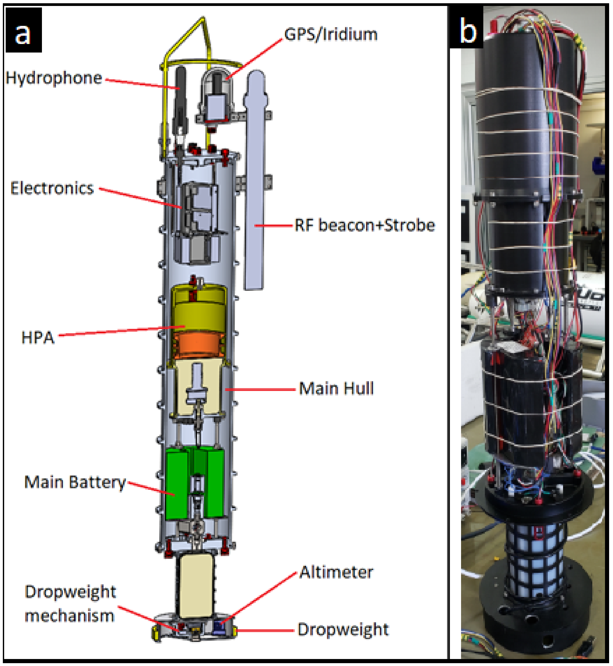
The float’s general arrangement is presented in Figure 5. The bottom endcap carries the VBE and main battery on a single lightweight support structure. The assembly process requires the bottom endcap to be inserted into the hull first and secured by fasteners. The electrical cabling of the bottom endcap assembly should be sufficiently long to protrude from the top of the hull to allow easy connection to the electronics module attached to the top endcap. After the wires are connected, they are laid on top of the HPA and the top endcap is inserted into position and secured by fasteners.

2.9. Hull Design

Based on the float components’ weight, dimensions and GA, the float hull could be sized. To accommodate the components in their proposed arrangement, a cylindrical pressure hull with an inner diameter of 150 mm and a minimum length of 800 mm was required. This pressure hull must meet two main requirements: first, it must withstand the hydrostatic pressure at a depth of 300 m; second, it must exhibit maximum Lagrangian characteristics. The second requirement can be translated into two mechanical properties: (1) thermal expansion and (2) compressibility. Since thermal expansion is a material property, the matching of the hull and water thermal expansions depends mainly on material selection. The coefficient of linear thermal expansion of aluminum is ${\alpha }_{Al}=24·{10}^{-6} \frac{1}{\mathrm{K}°}$ and its volumetric thermal expansion coefficient is ${\beta }_{Al}=75·{10}^{-6} \frac{1}{\mathrm{K}°}$. For the above float pressure hull, a coefficient of thermal volumetric expansion of approximately ${\beta }_F=7.2·{10}^{-5}\frac{1}{\mathrm{K}°}$ was computed—vs. that of sea water, which is ${\beta }_{SW}=21·{10}^{-7} \frac{1}{\mathrm{K}°}$ —resulting in a volume change of $1.23\frac{\mathrm{cc}}{\mathrm{K}°}$ and $0.0359\frac{\mathrm{cc}}{\mathrm{K}°}$ for the float’s hull and equal volume of water, respectively. Despite the significant difference between the two coefficients, due to the relatively shallow operational requirement and its subsequent small variations in temperature, aluminum 6061T6 was chosen as the hull construction material.

For the pressure hull, compressibility is not an inherent material property but rather a designed quantity, thus the pressure hull was designed with compressibility as close as possible to that of the local water column. Numerous local water column profiles of depth between 0 and 300 m were examined and an average water compressibility of ${\kappa }_w=4.2·{10}^{-5} \frac{1}{\mathrm{bar}}$ was determined. This value was set as the target compressibility for the float’s pressure hull.

A cylindrical pressure hull under external pressure can fail in one of two possible failure modes: static yielding or shell instability buckling. The hull thickness needed to withstand yield failure can be accurately calculated with analytical formulas, Lame’s equations and their derivatives. Analytical computation for the thickness required to avert buckling employs significant assumptions, resulting in less accurate calculations. Consequently, finite element analysis (FEA) is usually employed to achieve better accuracy. For thin-walled and long cylinders, the case for this hull design, static yield is usually the less stringent failure mode, albeit both failure criteria must be investigated.

First, the minimal wall thickness was calculated for both the cylindrical hull and the endcaps according to the static yield criterion. The calculation for the cylinder thickness Equation (6) is a derivation of Lame’s equations [21] with the thin-wall simplification $\frac{D_i}{t_{cyl }}>20$, where $t_{cyl }$ is the cylinder wall thickness and $D_i=150 \mathrm{mm}$ is the cylinder internal diameter. The thickness estimation for the endcaps is based on Equation (7) for a circular plate under distributed transverse loading with fixed boundary conditions [22].

$$t_{cyl}=\frac{\sqrt{3}}{4}\frac{P{D}_i}{{\sigma }_y}$$

(6)

$$t_{ec}=2{\left(\frac{3}{64}\frac{P{D}_i^2}{{\sigma }_y}\sqrt{1-\nu +{\nu }^2}\right)}^{0.5}$$

(7)

where $t_{cyl}$ and $t_{ec}$ are the cylinder and endcap wall thickness, respectively, and $D_i=150 \mathrm{mm}$ is the float’s internal diameter, ${\sigma }_y=275 \mathrm{MPa}$, E = 69 GPa and $\upsilon =0.33$ are the construction material’s (aluminum 6061T6) yield strength, modulus of elasticity and Poisson ratio, respectively, and $P=30 \mathrm{barg}$ is the hydrostatic pressure.

The minimum cylinder wall thickness for the shell instability buckling criterion was calculated by employing Equation (8), the David Taylor Model Basin formula [23]. This formula is suitable for thin walled near-perfect vessels. Here, in contrast to the static yield criterion, thin walled is defined as having a ratio of $\frac{D_i}{t_{cyl}}>60$, while near perfect refers to the absence of material and shape imperfections in the vessel’s shell.

$$P_{cr}=\frac{2.42E}{{\left(1-{\nu }^2\right)}^{0.75}}\left[\frac{{\left(t_{cyl}/D_i\right)}^{2.5}}{L/D_i-0.45{\left(t_{cyl}/D_i\right)}^{0.5}}\right]$$

(8)

where $L=850 \mathrm{mm}$ is the cylinder length and $P_{cr}$ is the critical buckling pressure.

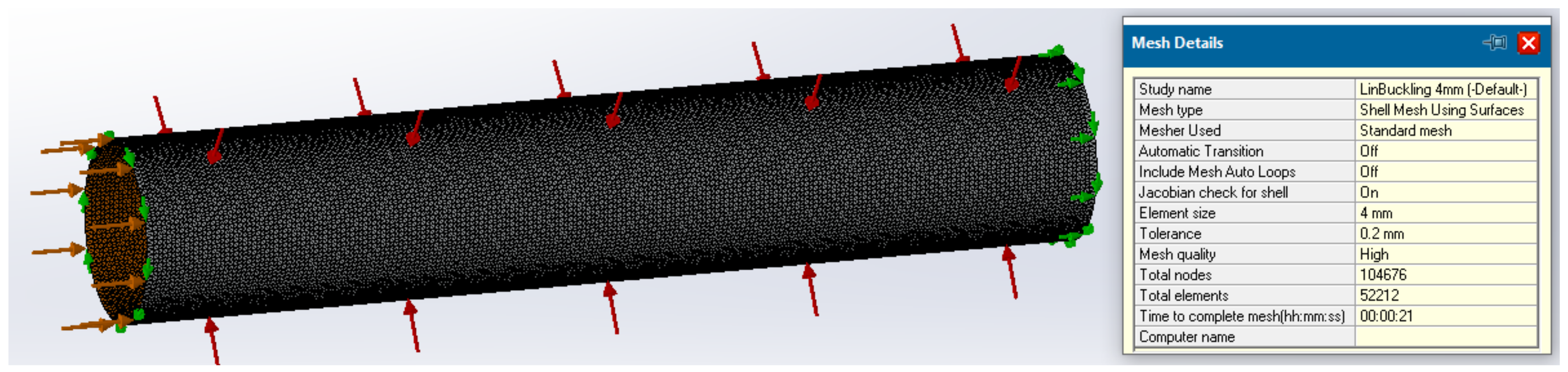
As previously mentioned, buckling formulas employ significant assumptions and approximations; for more accurate results of the buckling pressure or critical wall thickness, the use of FEA is recommended. FEA was performed using the commercial package SolidWorks Simulation. The FEA investigation comprised two analyses. The first was a linear buckling analysis that assumes small deformations and linear behavior of the material, i.e., the stress–strain relation, is represented by a constant modulus of elasticity, while the second FEA was a nonlinear one.

The linear analysis was employed to obtain a preliminary estimation for the buckling modes and critical buckling pressure. Figure 6 presents the analysis mesh and mesh details. For this FEA, the investigated model was the cylindrical portion 150 mm in diameter and 4 mm in thickness, without the endcaps. Shell elements, with an average size of 5 mm, were employed. Fixtures were defined in a polar coordinate system, with one end of the cylinder restrained from both rotation and axial displacement while, on the opposite end, only rotation was prevented. A hydrostatic pressure of 3 MPa was applied to the cylindrical face and an axial force of 58,800 N was applied to the free end to mimic the axial force produced by the hydrostatic pressure on the endcap.

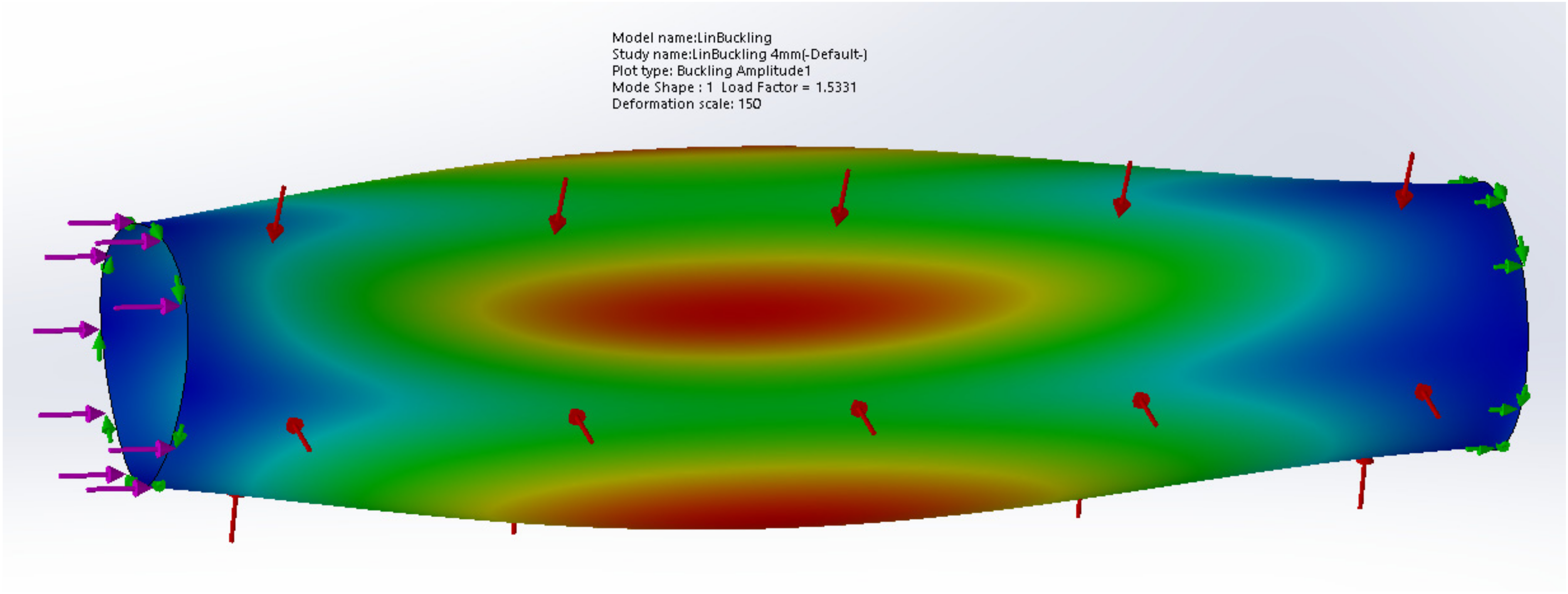
The analysis results are presented in Figure 7. The result of interest in this analysis is the “load factor”, which here has the same meaning as factor of safety (FOS). For the above-described model, a FOS against buckling equal to 1.53 was obtained, while it was defined that an $\mathrm{FOS}>3$ is desirable [24]. This increased FOS is taken to compensate for unavoidable geometrical imperfections and material nonlinearity, both of which may significantly lower the vessel’s buckling pressure [25]. An increase of wall thickness to 5.5 mm results in an adequate FOS of 3.3.

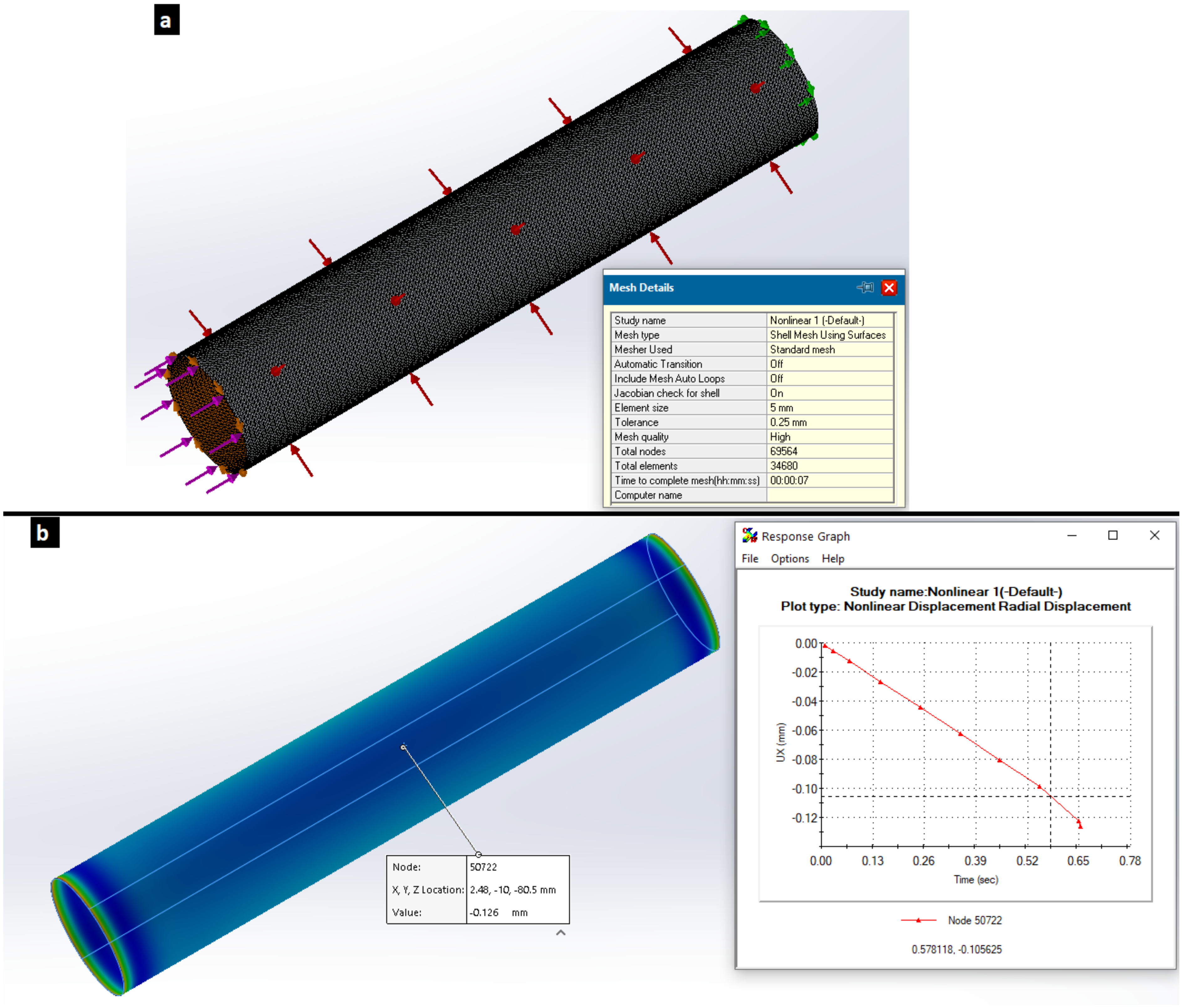
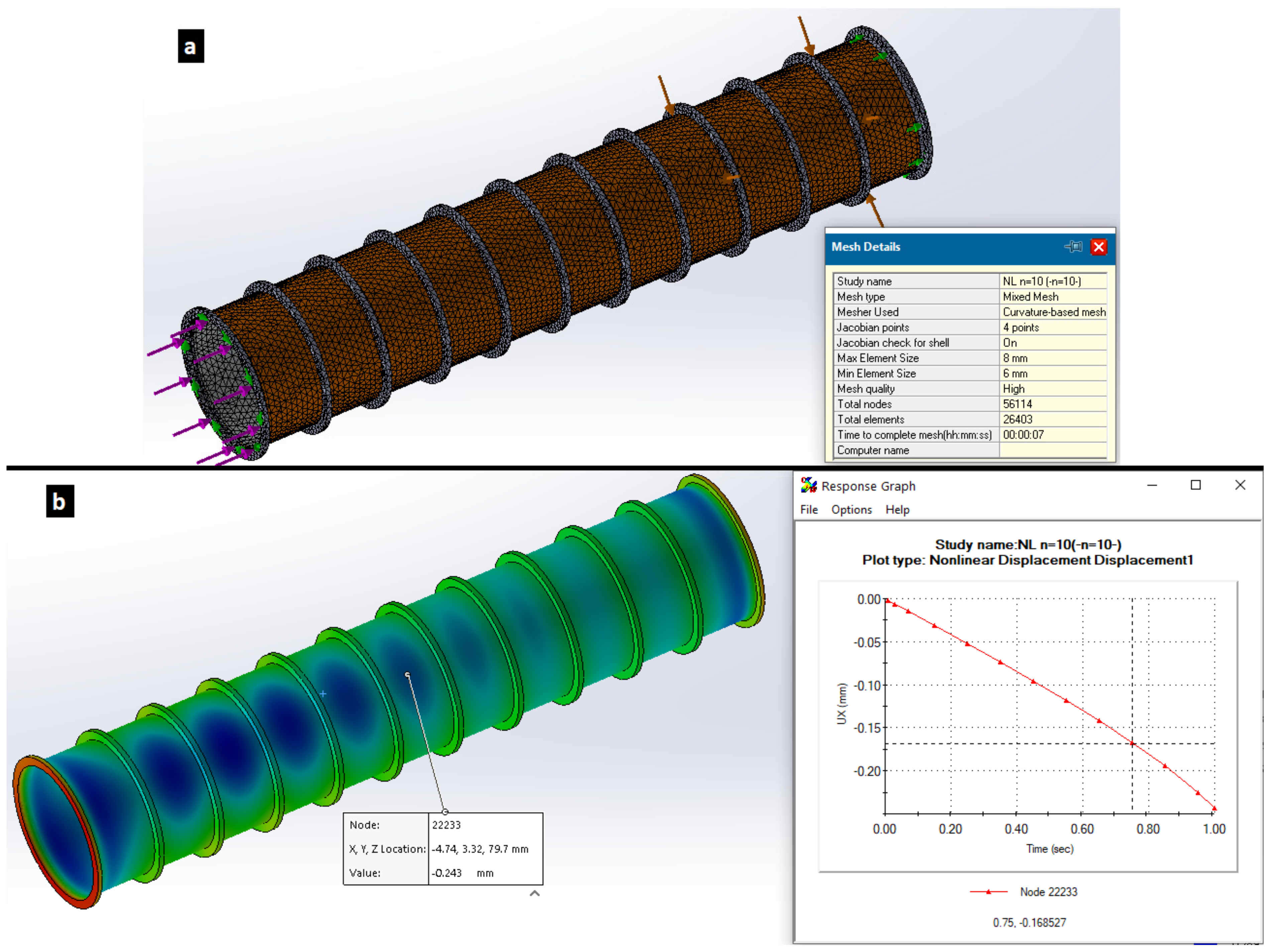
In addition, nonlinear static analysis was employed to consider nonlinearity in the material behavior, large displacements and contact between parts. For this analysis, the parameters of the model, meshing and fixtures were maintained almost identical to the linear analysis; only the mesh size was slightly increased due to computational constraints. The loads were applied in the same way as well, but instead of a constant value as in the linear analysis, the loads were defined as a linear ramp function with a value of zero at analysis pseudo time t = 0 and the maximum value at analysis end time t = 1. The results of the nonlinear analysis were interpreted in the following manner: for an arbitrary junction in the axial middle of the model, a plot of radial displacement vs. time was defined. The beginning of divergence of the radial displacement from linearity indicates the inception of buckling. Mesh, parameters and results of the nonlinear FEA are presented in Figure 8a and the results in Figure 8b. The chart in Figure 8b describes the arbitrary junction radial displacement versus pseudo time. Here, divergence occurred at approximately t = 0.6, yielding a buckling pressure of $P_{cr}=72 \mathrm{bar}$. The maximum deformation at the inception of buckling is presented in Figure 8b and equals 0.126 mm. Both the linear and nonlinear analyses predict a two-lobe buckling mode, but whereas the linear analysis yields a buckling pressure of 99 bar, the nonlinear analysis yields a buckling pressure of only 72 bar, well below the desired FOS of 3.

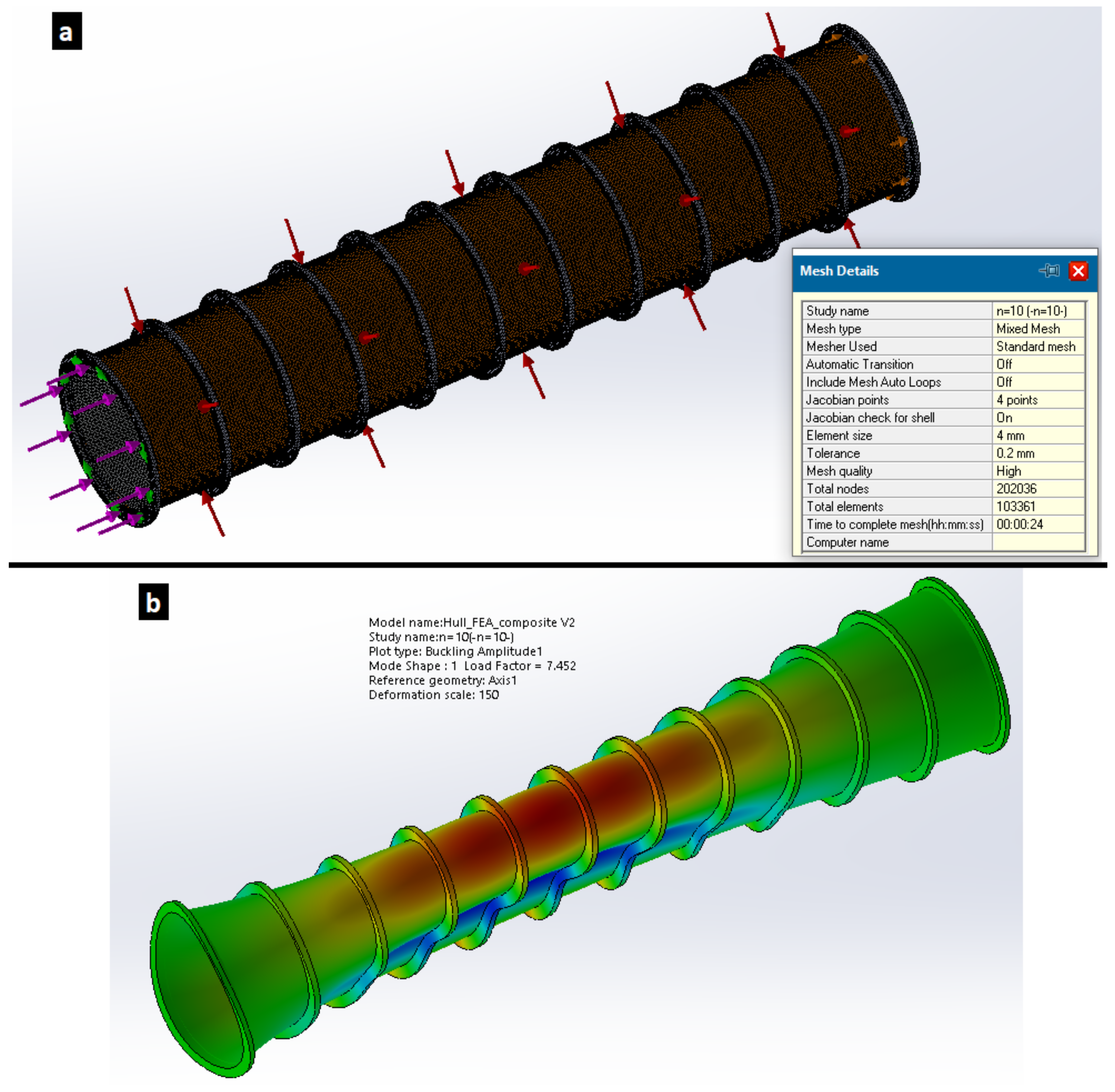
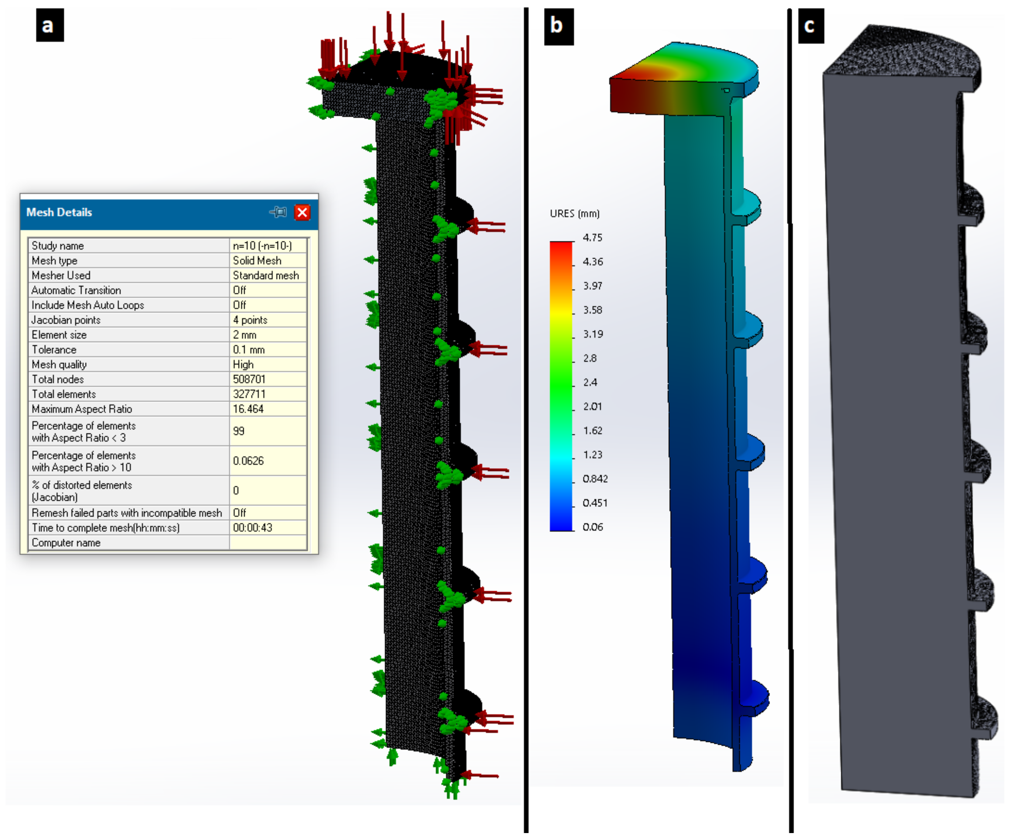
Based on the results of the simple cylinder FEA and in order to further increase the pressure hull’s FOS without a proportional weight penalty, it was decided to investigate a stiffened cylinder configuration. Equally spaced ring stiffeners were incorporated in the design on the external side of the cylinder. The endcaps were also augmented with perimeter and cross pattern stiffeners on the internal side. The endcaps were designed employing a standard static analysis for a target FOS of 3. The investigation of the stiffened cylinder followed a similar pattern to that of the plain cylinder. To facilitate an efficient analysis, the cylindrical portion of the hull was modeled with shell elements and the stiffeners with solid elements with a bonded connection between the two. A series of stiffeners and outer diameters were investigated with the maximum diameter set at 180 mm, the diameter of the endcap flange, until the target FOS was reached. Both linear and nonlinear analyses were performed. Figure 9 presents the stiffened cylinder linear analysis: Figure 9a displays the mesh, loads, boundary conditions and mesh details and Figure 9b shows the results, with an FOS of 7.45 achieved.

The nonlinear FEA analysis is presented in Figure 10: in Figure 10a, the mesh, loads, boundary conditions and mesh details are displayed; in Figure 10b, the analysis result is shown. The radial displacement diverges from linearity at t = 0.75, which translates into a pressure of 90 bar and the required FOS of 3, a much lower FOS compared to the 7.45 computed for the same configuration by the linear analysis.

Once the minimum hull strength requirement was met, the hull was investigated via static FEA for the target compressibility value. The three steps employed in the compressibility investigation—(a) meshing, (b) FEA and (c) deformed volume computation—are presented in Figure 11. Additional fine-tuning of dimensions was required to achieve the target compressibility. Due to symmetry, only $\frac{1}{8}$ of the model was employed. Following completion of the static FEA (Figure 10b), in order to measure the pressurized volume, the deformed model was exported to a SolidWorks part file. The compressibility was computed employing the formula:

$$\kappa =-\frac{1}{V}\frac{\mathrm{\Delta }V}{\mathrm{\Delta }P}$$

(9)

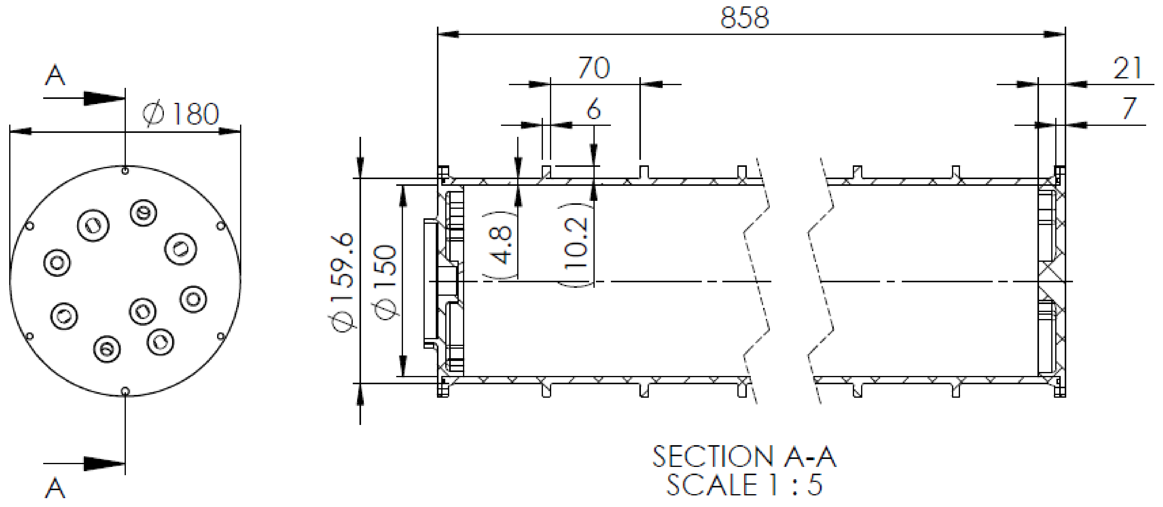
where $\kappa$ is the compressibility, $V$ is the initial volume and $\mathrm{\Delta }V$ is the change in volume due to the change in the applied pressure $\mathrm{\Delta }P$. Final hull geometry and main dimensions are presented in Figure 12.

3. Dynamic Model and Controller Design

The development of the equations of motion, and the subsequent dynamic model, is considered an essential part of this work, both for understanding the parameters driving the float motion and for the design of the motion controller. Since it is commonly accepted that horizontal motion of neutrally buoyant floats closely mimics the horizontal motion of water [9,26], only the vertical motion of the float was examined. In this direction, the equation of motion of the form of a forced harmonic oscillator, first proposed by [27] and later by [26], was used. The equation is developed for a neutrally buoyant float under forcing of isopycnal movement and considers compressibility, thermal expansion, drag and added mass. Here the quadratic drag component Equation (10) is augmented with the linear drag component $F_{D_{lin}}$ proposed by [28], represented by Equation (11), arising from self-induced internal waves caused by the passage of the float through stratified water.

$$F_D=\frac{1}{2}{\rho }_w{C}_{D}A\left|\frac{d{\varsigma }_r}{dt}\right|\frac{d{\varsigma }_r}{dt}$$

(10)

$$F_{D_{lin}}={\rho }_{w}ANL\frac{d{\varsigma }_r}{dt}$$

(11)

where ${\rho }_w$ is the water density, $C_D$ the drag coefficient, $A$ the float cross-section area, $N$ the buoyancy frequency and $L$ the float length scale, which is related to the float radius. $\frac{\partial {\zeta }_r}{\partial t}$ is the vertical velocity of the water relative to vertical velocity of the float. The relation of $L$ to the float geometry is, as yet, inconclusive, but for a float with a drogue of $r=0.7 \mathrm{m}$ in radius, $L$ was empirically shown to be 1.1 m or $L=1.57r$ [28]. Similar ratios of $\raisebox{1ex}{$L$}\!\left/ \!\raisebox{-1ex}{$r$}\right.$ were used in the simulation. The equation of motion is presented in Equation (12).

$$\frac{d^2{\varsigma }_r}{d{t}^2}+\sigma \frac{d{\varsigma }_r}{dt}+{\omega }_0^2{\varsigma }_r={\omega }_1^2{\varsigma }_w$$

(12)

The resulting equation of motion is very similar in form to the equation of a harmonic oscillator under base excitation. From the comparison of the equation of motion to the standard form of the equation of a harmonic oscillator, several conclusions are immediate: $\sigma$ (Equation (12)) is a term representing the dissipation of energy due to various damping mechanisms; ${\omega }_0$ (Equation (13)) is the natural frequency of the float, i.e., the free oscillation frequency of the float as a result of initial displacement from its equilibrium isopycnal; and ${\omega }_1$ (Equation (14)) does not have an analogue in the harmonic oscillator equation. Here, it is related to adiabatic effects on the buoyancy force per unit mass. The coefficients of Equation (11) are given by Equations (13)–(15):

$$\sigma =\left(NL+\frac{1}{2}{C}_D\left|\frac{d{\varsigma }_r}{dt}\right|\right)\frac{1}{L_f\left(1+\vartheta \right)}$$

(13)

$${\omega }_0^2=\left[{\rho }_0{g}^2\left({\kappa }_w-{\kappa }_f\right)+N^2-{\beta }_{f}g\frac{d{T}_w}{dt}\right]\frac{1}{1+\vartheta }$$

(14)

$${\omega }_1^2=\left[{\rho }_0{g}^2\left({\kappa }_w-{\kappa }_f\right)+{\beta }_{f}g\frac{d\mathrm{\Theta }}{dz}\right]\frac{1}{1+\vartheta }$$

(15)

where $Z_0,Z_w,Z_f$ represents the float’s equilibrium isopycnal depth, current isopycnal depth and current float depth, respectively; ${\zeta }_w=Z_w-Z_0$, ${\zeta }_f=Z_f-Z_0$ are the water and float displacements relative to the equilibrium depth, respectively; ${\zeta }_r=Z_w-Z_f$ is the relative water to float displacement and $\frac{\partial {\zeta }_w}{\partial t},\frac{\partial {\zeta }_f}{\partial t}$ are the water and float vertical velocities, respectively; ${\rho }_0$ is the equilibrium density, $\vartheta$ is the normalized added mass, $g$ is the acceleration of gravity and $T_w$ and $\mathsf{\Theta }$ are the water temperature and adiabatic temperature, respectively; ${\kappa }_w$ and ${\kappa }_f$ are the water and float compressibility, respectively; ${\beta }_f$ is the float coefficient of thermal expansion and $L_f$ is the float length.

Table 3. Dynamic model constants.

$L$	Float Length Scale	140 mm
$C_D$	Axial drag coefficient	0.81
$L_f$	Float length	1000 mm
ϑ	Normalized added mass	1
${\beta }_f$	Float coefficient of thermal expansion	$7.2·{10}^{-5}\frac{1}{\mathrm{K}°}$
κf	Float compressibility	$4.2·{10}^{-5} \frac{1}{\mathrm{bar}}$

summarizes the various constants employed in the dynamic model.

For the development of a dynamic model from the above equations, the MATLAB Simulink environment was employed. The dynamic model incorporates the water column properties, water motion forcing, the equation of motion, the augmented PID control scheme, the pump flowrate and power curves as a function of the internal HPA pressure and external water pressure and bladder inflation. The water column properties were taken from actual local CTD deployments in the EMS performed during different months, covering all seasons. The forcing water motion was constructed following IW linear theory [29]; wave amplitude and numbers can be selected freely by the user. The dynamic model requires the selection of two initial conditions: (1) float depth ${\zeta }_f\left(t=0\right)$ and (2) float vertical speed $\frac{\partial {\zeta }_f}{\partial t}\left(t=0\right)$. The relevant oceanographic conversions were performed employing the TEOS-10 /GSW MATLAB toolbox [30].

The float’s motion closed loop control is performed by a PID controller. While PID is not optimal for float motion control [31], it was selected here due to its simplicity and capability to achieve adequate, if not perfect results. The developed controller comprises two sub controllers; one to handle the pressure seeking mission and a second to handle the density seeking mission. The following description refers to the pressure controller, with the density controller being analogous with the difference that, for the density controller’s derivative term (D), the pressure error was used instead of the density error. This was done to avoid the use of the highly noisy density derivative and deemed acceptable since both values are related to the speed of the float.

Simulations have enabled several enhancements to the classic PID scheme: (1) Two sets of coefficients were defined for the PID controller. The first set consists of only the proportional coefficient. It is used when the error is larger than a predefined threshold value, usually set between 5–10 dbar. Once the error is within the threshold, the PID coefficients are switched to a full set of PID or PD coefficients. The purpose of this is to ensure that the start of the float motion is achieved as quickly as possible, e.g., submersion from the surface. (2) Use of decreasing actuation times of the pump with the decrease of the error in conjunction with decreasing duty-cycle; this is to say that as the float approaches the setpoint, the pump is turned on for increasingly shorter bursts with increasing off times in-between. This is conducted via linear interpolation between the error (0, 10) dbar, the pump actuation time (0.5, 5) s, (0.5 s being the mechanical minimum actuation limit of the pump) and the duty cycle (0.05, 1). For example, when the float just passes the threshold, the ON time is 5 s and the duty-cycle is 100%, with the resulting OFF time being 0, meaning the pump runs continuously. When the error approaches 0, ON time is 0.5 s, the duty-cycle is 5% and the resulting OFF time, the pause between pump actuations, is 99.5 s. This is done to compensate for the great difference between the pump and the float response times, i.e., allowing sufficient time for the float motion to respond to the change in the bladder volume.

The Simulink model is constructed of several separate sub-blocks. The water profile data are preprocessed and loaded into the model workspace upon opening. The blocks comprising the model are as follows: (1) Internal wave generator: this block computes the four IW equations according to the linear wave theory with its output providing the water motion and pressure and density perturbations. (2) Equation of motion: this block computes the equation of motion of the float; its output is the float’s state vector (acceleration, velocity and displacement). (3) Sensor block: this block produces the ambient water parameters from the water profile data according to the current float depth and adds noise. (4) Motion controller block: this block realizes the augmented PID motion controller. Its output is the pump control voltage in percentages between 40% and 100%. (5) Volume calculator block: this block applies the pump flowrate curve according to the PID output and the pressure balance on the pump and changes the bladder volume accordingly. Finally, (6) is the power calculator block that applies the pump power curve according to the pressure and flowrate of the pump and accumulates the consumed energy

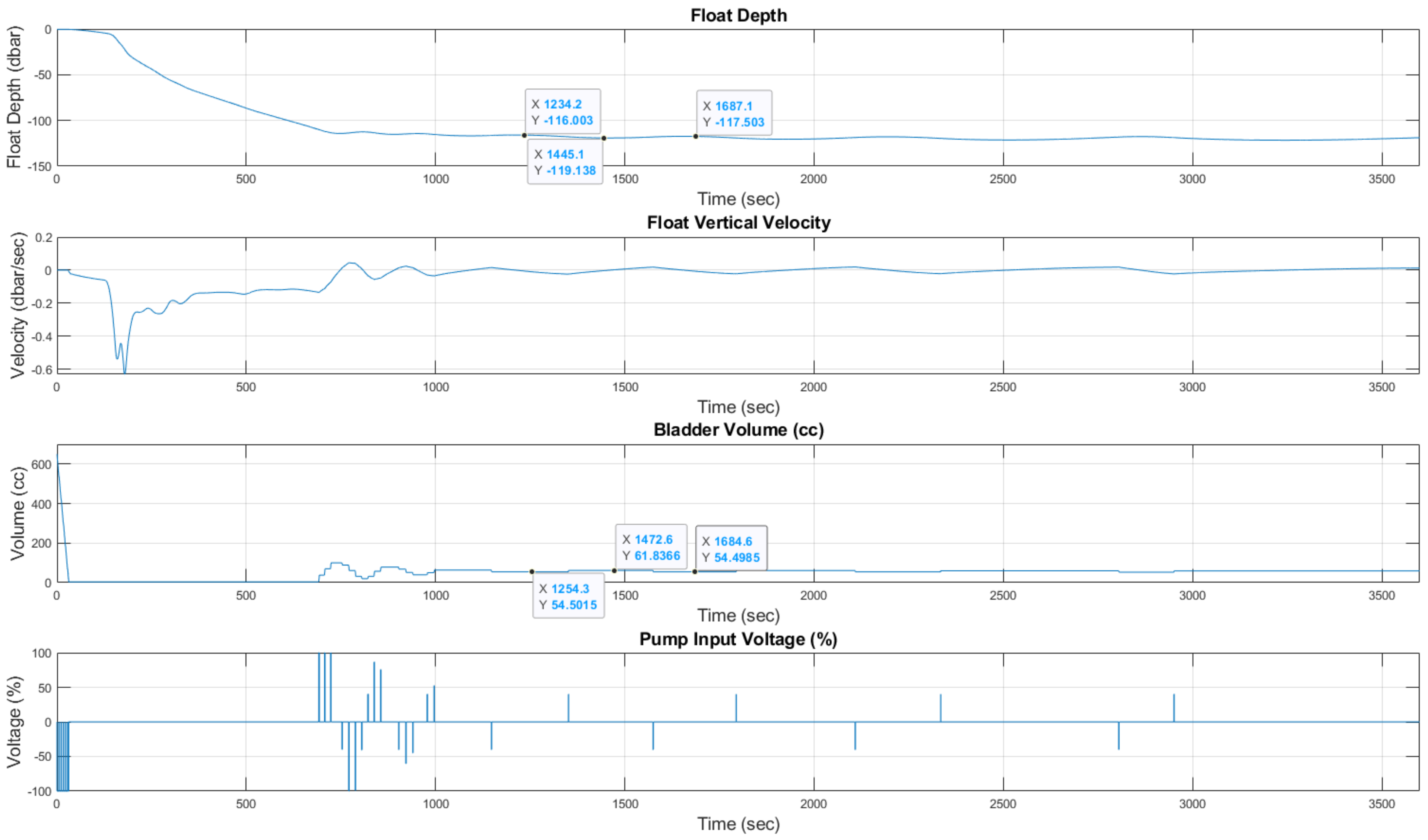
All desired results including water and float motion, bladder and float volume, instantaneous and accumulated power drawn, etc., can be displayed as charts. Figure 13 presents a sample simulation of the float released from the surface with initial bladder volume of 650 cc and a pressure setpoint equal to 120 dbar. The results are presented in charts displaying float depth, float velocity, bladder inflation and pump control voltage. As can be seen in Figure 13, the float depth fluctuates between 117.5 and 119 dbar, while the bladder volume fluctuates between 61 and 54.5 cc. A bladder volume of 57.85 cc would bring the float to neutral buoyancy at the setpoint depth.

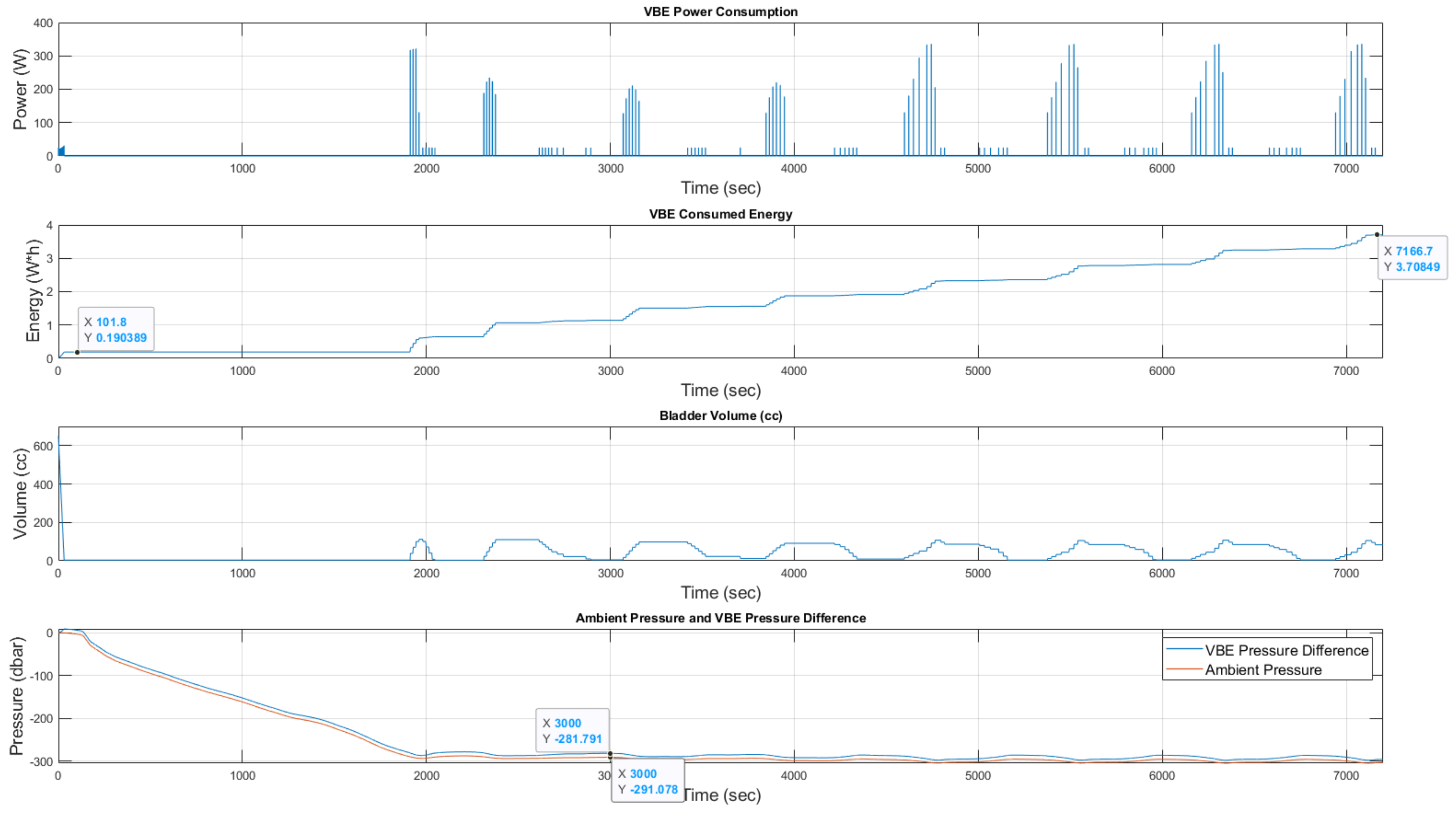
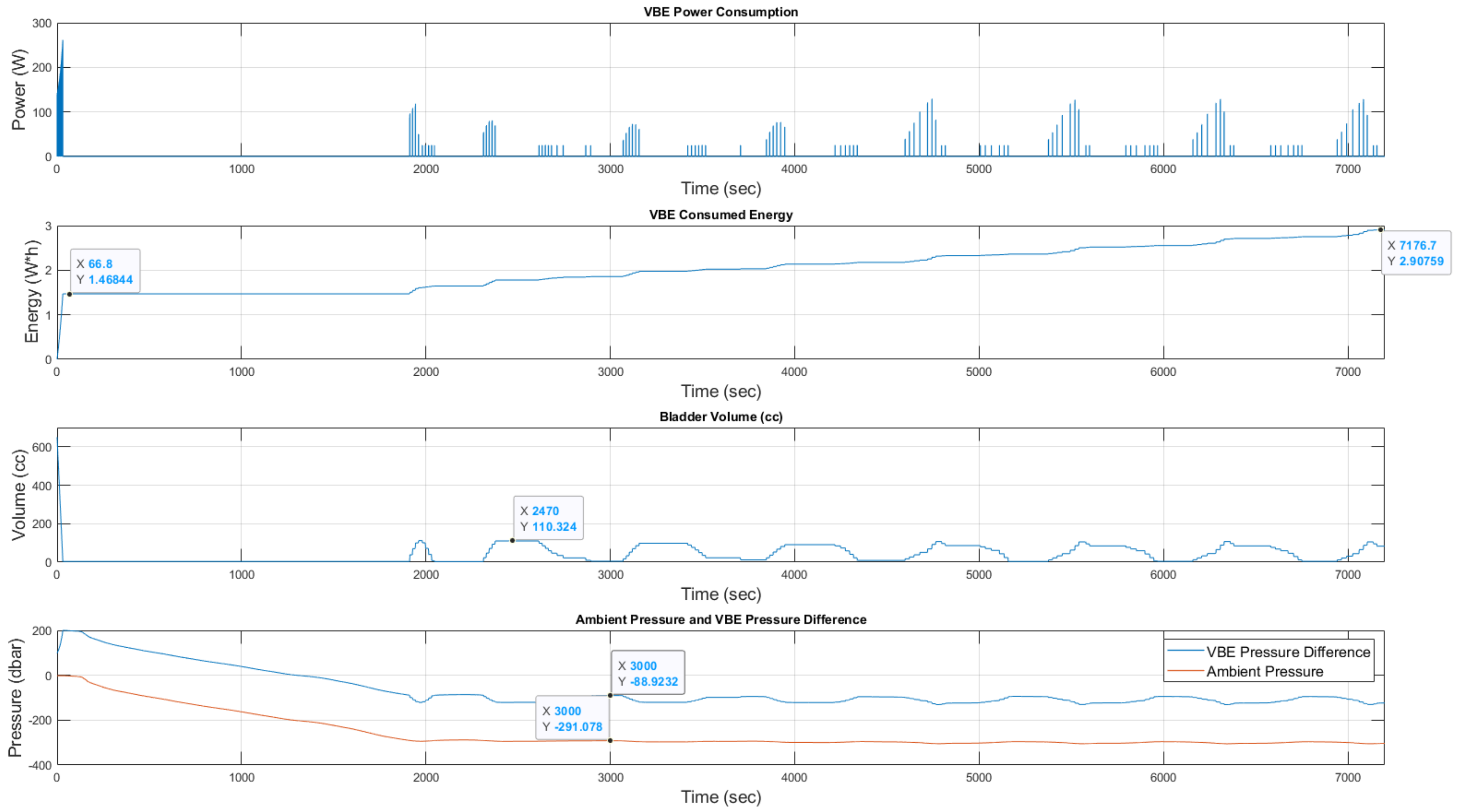
To emphasize the power consumption advantage of the pressure assistance concept, Figure 14 and Figure 15 present the results of two simulations where a float with a full 650 cc bladder is released from the surface with a pressure setpoint of 300 dbar. At the 300 dbar depth, an IW with amplitude of 10 m and cycle time of 785 s is generated. The only difference between the two simulations is the nitrogen initial filling pressure of the HPA; in simulation #1 (Figure 14), the HPA filling pressure (when the bladder is full of oil) is 0 barg, i.e., there is no pressure assistance, whereas in simulation #2 (Figure 15), the HPA filling pressure is 10 barg. Figure 14 and Figure 15 present, from top to bottom, the VBE power draw, consumed energy, bladder volume, ambient hydrostatic pressure and pressure difference across the VBE pump.

The energy required to initially empty the bladder and commence submergence is 0.19 Wh and 1.47 Wh for simulations #1 and #2, respectively. At approximately t = 1900 s, the controller engages to stabilize the float against the IW. At the end of 2 h simulation, the energy consumed by the VBE is 3.7 Wh and 2.9 Wh for simulations #1 and #2, respectively. Discounting the energy required for the initial submergence, the values are 3.51 Wh and 1.43 Wh for simulations #1 and #2, respectively. Hence, for a 24 h mission to a depth of 300 m, approximately 1 h would be spent profiling to the setpoint depth and back to the surface. The remaining 23 h would require approximately 54 Wh and 22 Wh for a standard VBE and pressure assisted VBE, respectively, resulting in a 60% reduction in the consumed energy. For eventual inflating of the bladder and surfacing the energy consumed will be 2.9 Wh and 1.45Wh, bringing the total mission energy consumption to 57 Wh and 25 Wh for the non-assisted and pressure assisted VBEs, respectively.

4. Software

Controllers’ Code

The Pi code is a state machine code that moves from state to state as prescribed in the mission profile and jumps to a non-nominal or emergency state in response to a flag raised by the safety agent running in the background. The Pi and Mega simplified algorithms are presented in Figure 16 and Figure 17, respectively. The Pi, upon switching on the power, undergoes mission prep states (#3–#5, Figure 16), which can be skipped depending on the mission profile. The first mandatory state is the water identification state (#6), where the bottom pressure sensor’s readings are monitored to identify submergence. As soon as water is identified, the mission commences, sensor data from the Mega are gathered (#8), checked for emergency flags (#9), logged (#11) and provided to the motion controller (#12). The Mega constantly transmits data to the Pi, while the Pi only transmits back when the data are non-zero. If an emergency is detected by the Mega or Nano safety agents, appropriate action is taken by the Pi and the mission is aborted, either triggering a normal abort (normal surfacing) or an emergency abort (DW release and surfacing). At nominal operation, the “receive data-compute-transmit data” (#8–#13) loop is repeated until the mission is completed. When the underwater mission is completed (currently, mission completion is time based), the state is changed, normal surfacing (#16) is initiated and, upon identification of atmospheric pressure (#17), the beacons are enabled (#18).

The Mega code, Figure 17, scans all sensors, starting with the leak sensors (#2). If a leak is detected, it first initiates surfacing (#3) and then transmits an appropriate flag to the Pi. At nominal operation, all sensor data are transmitted to the Pi. If no incoming flags (#5 and #7) or a full complement of pump actuation parameters (#9) (voltage, direction, and actuation time) are identified, the sensors’ “read and transmit” loop runs continuously. Except in case of leak detection, when the Mega takes action independently of the Pi (#2–#3), the Mega serves as a data conduit between the Pi and the instruments.

5. Float Testing

The float testing was conducted incrementally, increasing in difficulty starting at our facility (dock trials) and followed by sea trials.

5.1. Dock Trials

Firstly, to validate the mechanical design, as well as validate watertightness and hull integrity, pressure tests to 25 barg were conducted in our pressure chamber. In parallel, a number of comprehensive pump functionality tests were conducted, including a test to start up the pump against high pressure and a test to estimate the effective minimal time the pump may be turned on before it is turned off. Following the initial tests, tabletop Arduino and Pi code was validated using simulated pressure input to the PID controller to monitor the output command to the pump. Once tabletop code verification had been completed, pool tests were conducted in the facility’s 2.5 m-deep pool. These tests were a miniature version of a real mission, in which the float was required to identify water, submerge, wait on the bottom, surface, identify air and initiate Iridium communication for retrieval. To verify the float’s endurance, a looping test sequence was performed repeatedly until the batteries were depleted. Several pool depth-keeping tests were performed as well, with the float maintaining a 1.5 m depth with 0.2 m amplitude oscillations.

Tests were performed in the pressure chamber to verify the operation of the VBE in dual-directional modes, both against HPA and against external hydrostatic pressure. A final test was conducted in the pressure chamber for testing and qualifying the DW release mechanism at the depth pressure. Finally, pool experiments were conducted for all scenarios under fully autonomous conditions. Figure 18 shows the float as it was tested in the pressure chamber and in the pool.

Following completion of all the described dockside testing, sea trials were conducted.

5.2. Sea Trials

The Alpha trial consisted of three deployments at shallow depth. All deployments were in pressure-keeping mode for a predefined duration, with the pressure-keeping timer set to start when the float passed the 0.4 dbar proximity mark to the setpoint. During the first two deployments, the float was untethered and supervised by divers, while during the final deployment, the float was unsupervised and tethered to a surface buoy. On the third deployment, due to very strong currents and the resulting tension of the tether, the float was unable to reach the setpoint depth. As a result, the measurements taken are not presented here.

Table 4. Deployment parameter summary.

Deployment	Setpoint (dbar)	Time on Setpoint (min)	Repetitions
#1	10	10	1
#2	12	2	2

summarizes the parameters of the first two deployments. Each surfacing was followed by iridium transmission.

The results of deployments #1 and #2 are presented in Figure 19 and Figure 20, respectively. Figure 18a and Figure 19a present the mean pressure, i.e., the averaged reading of the four external pressure sensors and Figure 18b and Figure 19b show the calculated bladder volume, as laid out in Section 2. These first two deployments were successful, with the float reaching its target depth, stabilizing, surfacing and achieving iridium transmission within seconds of transmission initiation. The areas marked in red in Figure 18a and Figure 19a show no change in pressure despite a change in bladder volume. This is a result of an oversight in the code where during the pump actuation for full surfacing, the navigational sensors were not logged. For the initial trials, while the pump is active, the Mega reads only pump RPM and the two HPA sensors. Since maximum pump actuation time is 5 s and sampling of all sensors is renewed as soon as the pump stops, this practice is sufficient for initial trials.

When examining the results of deployment #1 (Figure 19), it becomes apparent that the derivative term of the PID controller was too strong. When submerging for the first time, there was a sharp upward correction around 7.1 dbar, followed by a series of smaller corrections due to the dominance of the PID controller’s derivative term. At approximately t = 577 s, the float passed the 0.4 dbar threshold to the set point and began oscillations of approximately 0.4 dbar in amplitude at a depth of approximately 9.4 dbar until end of the mission; surfacing was initiated at approximately t = 1173 s. In the pressure-keeping mode, the bladder volume fluctuated between 40 and 106 cc, while, per the computed model, a volume of approximately 79 cc was required for neutral buoyancy.

When examining the results of deployment #2 (Figure 20), similar behavior to deployment #1 is observed. Again, when submerging for the first time, a series of upward corrections were made as a result of a too dominant derivative term. At approximately t = 414 s, the float stabilized and began small cyclic oscillations of approximately 0.15 dbar near the 12 dbar setpoint. On the second dive, the float reached the setpoint much more quickly, with only three and less prominent upward corrections. The reason for the difference in diving behavior between the two dives is unclear, and further testing is required.

In Figure 21a, the float is seen just before ascent at the end of the first deployment and in Figure 21b, the float is seen on the sea surface after surfacing at the end of the first deployment.

6. Conclusions

In this paper, we describe the complete process of designing and developing an enhanced, low-cost Lagrangian float suitable for deployment in littoral regions to depths of 300 m. An in-depth description of all development steps along with the testing procedure and the results of the first sea trial is provided. The work describes in detail the development of the Lagrangian hull, a novel pressure assisted VBE design and an innovative compact drop-weight mechanism.

Near term future work includes the fine-tuning of the PID controller and extensive float deployments in the EMS in search of IW. As part of these missions, a comparison of the noise output and energy consumption of VBE, operating at different depths with and without pressure assistance, will be conducted. Longer term work will include the acquisition of accurate float parameters and the extension of the dynamic model. Still longer-term plans include the extension of the float code to include new mission profiles, e.g., altitude keeping. The incorporation of onboard ground-truth instrumentation for accurate measurement of both float and surrounding water velocities to enable the verification of Lagrangian behavior is also planned.