Dual-Algorithm Hybrid Method for Riser Structural Health Monitoring Using the Fewest Sensors

Abstract

This study suggests a novel riser structural health monitoring methodology based on a dual algorithm (DA). In this method, the displacement tracing algorithm first traces the node displacement and tension up to the last sensor position called the target point. Then, the movement and tension at the target point are used for boundary conditions of the finite element (FE) simulator to obtain displacements and stresses below the target point. The developed method is validated through numerical simulations by comparing riser behaviors/stresses from the fully coupled model with those from the proposed method with numerical sensors. For that, a moored FPSO (floating production storage offloading) system with SCR (steel catenary riser) or SLWR (steel lazy-wave riser) is employed. Only three angle sensors are used at the top portion to monitor the entire length of riser. Much simpler forced top oscillation method is also investigated, which only uses riser top movement for running FE simulator, which cannot accurately reproduce the dynamics of the upper portion of riser since real-time wave action is ignored. The developed DA riser monitoring methodology can reproduce the movements and stresses along the entire length within around 5% error regardless of riser shapes and materials.

1. Introduction

Nowadays, the demand for global energy keeps increasing due to world economic growth. Despite more use of renewable energy, the supply of oil and gas is still important. In particular, offshore platforms continue to produce a good portion of the entire oil and gas. For safety and prevention of spills, the structural integrity of production riser (elastic pipeline to transfer oil and gas from well to platform) and mooring system is considered to be highly important [1,2,3]. Thus, many researchers try to develop a robust approach for monitoring risers by using sensors and ROVs (remotely operated vehicles) [4].

The ROV method is only intermittent and very expensive compared to the sensor-based method. The sensor-based method can be real-time monitoring if sensor signals can be obtained in real time [5]. Additionally, if the riser profile can be traced, accumulated fatigue damage can be assessed simultaneously, which is very important for the life extension of the system.

Based on this background, researchers have paid more attention to sensor-based monitoring methods. For example, Ziegler and Muskulus [6] investigated sensor-based monitoring approaches using accelerometer, inclinometer, and strain gauges. Additionally, Karayaka et al. [7] researched localized-strain and dynamic-response measurements. The sensor-measurement strategies in the scaled model tests of floating wind turbines and wave energy converters were investigated by O’Donnell et al. [8]. While Li et al. [9] developed an acoustic telemetry scheme for the estimation of riser accumulated fatigue by VIV (vortex-induced vibration). Additionally, McNeill et al. [10] introduced the use of combining acceleration and angular information to the decision-making process for quasi-static angles along the riser. A new technology based on optical fiber sensors with wire to transmit measured strain data was proposed by Morikawa et al. [11]. Additionally, Peng and Zhi [12] demonstrated the strengths and weaknesses of various structure health monitoring methodologies including sensing technology. Kim et al. [13] used numerical simulations with numerical sensors and OMA (operational modal analysis) for the structural health monitoring of floating wind turbines. Additionally, Chung et al. [14], Chung et al. [15], Chung et al. [16], Kim et al. [17], and Kwon et al. [18] developed several methods to trace the real-time profile, tension, and bending moment of riser/tendon by using a series of numerical bi-axial inclinometers or accelerometers [19] along the line. Furthermore, allowable tendon stress under stochastic excitation was studied [20]. Continuously, the ultrasonic approach using voltages, time, and various other factors was also adapted to structural health monitoring [21,22,23,24,25]. As a new approach, the magnetic flux leakage method, which can only detect damage, was emerged recently [26,27].

The real-time power/data transmission to/from the deep portion of a riser without electric/optical wire can be challenging. In this case, acoustic data transmission can be employed [9]. Jahangiri et al. [28] evaluated the power-supplying method using piezoelectric energy converters for subsea sensors. Optical signals [4,29] can be used for data transmission if distance and water visibility are acceptable. The easiest and cheapest method is data transmission through electrical/optical wire in real time if sensors are located close to the water surface. In this case, a continuous power supply can also be easily achieved. Then, a question may arise: “can we use only a couple of sensors near the free surface and still trace/monitor the behavior of the remaining deep portion of riser?”. If this is possible, it can be the cheapest and simplest riser monitoring method, especially in deep water. This paper addresses this issue.

To meet the objective, one approach is based on using machine learning (ML) algorithms with a minimum number of sensors [18,30]. Alternatively, a hybrid method using a dual algorithm (DA) based finite element (FE) simulator with a couple of physical sensors can be employed, which is addressed in this paper. The basic assumption of the DA approach is that the FE riser simulator is good enough to reliably represent the actual riser behavior [31,32]. The developed method can also be straightforwardly applied to mooring lines, umbilical, power lines, and any other elastic lines.

In this regard, a real-time riser structural health monitoring method based on the DA approach using a minimum number of inclinometers (attached to the top portion of riser) is investigated. First, a general theory for the riser tracing algorithm and FE simulator is briefly explained. Then, the applied DA model with numerical inclinometer signals is described. To validate the developed methodology, an FPSO (floating production storage offloading) system at 1000 m water depth with SCR (steel catenary riser) or SLWR (steel lazy-wave riser) is modeled, and the developed algorithms are applied for 1-year and 100-year storm conditions. Then, the estimated and actual riser dynamic behaviors are compared. A simpler method, forced top oscillation (FTO), using only the movements of the riser top point, is also introduced and compared with the presently proposed method.

Again, the objective of this paper is to introduce a novel approach to monitor the behavior of riser and its stress with several sensors near free surface using the DA hybrid method. The contents of this study are as follows. Through Section 2 and Section 3, DA (node displacements tracing using quadratic interpolation function and 3D curve length equation and tension and bending-moment estimation) are more explained. Continuously, in Section 4, the DA hybrid method for riser structural health monitoring using the fewest sensors is explained in detail. Additionally, the numerical setup for the target structure (FPSO with SCR and SLWR at 1000 m water depth) and environmental conditions (1 yr-normal operating and 100 yr-extreme storm conditions) are summarized in Section 5. Section 6 presents structure health monitoring results and discussions. Finally, conclusions and future work are presented in Section 7 and Section 8. Again, this paper presents an innovative structure health monitoring methodology based on the suggested dual use of node displacement/tension tracing algorithm and FE simulator.

2. Riser Profile Tracing Algorithm

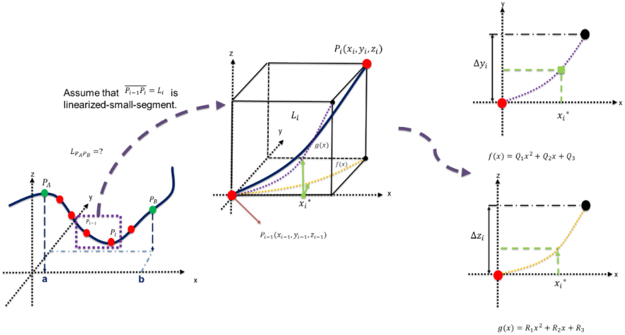
First, to trace the riser profile up to the target point to subsequently run the FE simulator, the riser-profile-tracing algorithm needs to be developed. The given information is the moving top point and values measured by angle sensors at the respective sensor locations. Still, another information has to be used, which is the curved line length in 3D space between the sensor points. This is explained in the following with Figure 1.

Here, the entire curved line length in 3D space ($L_{P_A{P}_B}$) between the two sensor endpoints can be calculated by the summation of numerous small-segment ($L_i=P_{i-1}{P}_i$) lengths:

$${\mathrm{L}}_{{\mathrm{P}}_{\mathrm{A}}{\mathrm{P}}_{\mathrm{B}}}={{\displaystyle \sum }}_{\mathrm{i}=1}^{\mathrm{n}}\left|L_i\right|={{\displaystyle \sum }}_{\mathrm{i}=1}^{\mathrm{n}}\left|{\mathrm{P}}_{\mathrm{i}-1}\right.\left.{\mathrm{P}}_{\mathrm{i}}\right|$$

(1)

$${\mathrm{L}}_{\mathrm{i}}=\left|{\mathrm{P}}_{\mathrm{i}-1}\left.{\mathrm{P}}_{\mathrm{i}}\right|=\right.\sqrt{{({\mathrm{x}}_{\mathrm{i}-1}-{\mathrm{x}}_{\mathrm{i}})}^2+{({\mathrm{y}}_{\mathrm{i}-1}-{\mathrm{y}}_{\mathrm{i}})}^2+{({\mathrm{z}}_{\mathrm{i}-1}-{\mathrm{z}}_{\mathrm{i}})}^2}=\sqrt{{({\mathsf{\Delta }\mathrm{x}}_{\mathrm{i}})}^2+{({\mathsf{\Delta }\mathrm{y}}_{\mathrm{i}})}^2+{({\mathsf{\Delta }\mathrm{z}}_{\mathrm{i}})}^2}$$

(2)

By using the decomposed quadratic interpolation functions for y and z locations (f(x), g(x)) in the x-y and x-z planes (Figure 2) and mean value theorem (Equation (3)), the small segment length equation (Equation (2)) can be re-written as (Equation (4)):

$${\mathsf{\Delta }\mathrm{y}}_{\mathrm{i}}={\mathrm{f}}^{\prime }\left({\mathrm{x}}_{\mathrm{i}}{}^{*}\right)·{\mathsf{\Delta }\mathrm{x}}_{\mathrm{i}},{\mathrm{where}\mathrm{x}}_{\mathrm{i}}{}^{*}\mathrm{in}\left[{\mathrm{x}}_{\mathrm{i}-1},{\mathrm{x}}_{\mathrm{i}}\right],{\mathsf{\Delta }\mathrm{z}}_{\mathrm{i}}={\mathrm{g}}^{\prime }\left({\mathrm{x}}_{\mathrm{i}}{}^{*}\right)·{\mathsf{\Delta }\mathrm{x}}_{\mathrm{i}},$$

(3)

where ${\mathrm{x}}_{\mathrm{i}}{}^{*}\mathrm{in}\left[{\mathrm{x}}_{\mathrm{i}-1},{\mathrm{x}}_{\mathrm{i}}\right]$,

$$\left|{\mathrm{P}}_{\mathrm{i}-1}\left.{\mathrm{P}}_{\mathrm{i}}\right|=\right.\sqrt{{({\mathsf{\Delta }\mathrm{x}}_{\mathrm{i}})}^2+{({\mathsf{\Delta }\mathrm{y}}_{\mathrm{i}})}^2+{({\mathsf{\Delta }\mathrm{z}}_{\mathrm{i}})}^2}=\sqrt{{({\mathsf{\Delta }\mathrm{x}}_{\mathrm{i}})}^2+{({\mathrm{f}}^{\prime }\left({\mathrm{x}}_{\mathrm{i}}{}^{*}\right)·{\mathsf{\Delta }\mathrm{x}}_{\mathrm{i}})}^2+{({\mathrm{g}}^{\prime }\left({\mathrm{x}}_{\mathrm{i}}{}^{*}\right)·{\mathsf{\Delta }\mathrm{x}}_{\mathrm{i}})}^2}$$

(4)

where ${\mathrm{x}}_{\mathrm{i}}{}^{*}\mathrm{in}\left[{\mathrm{x}}_{\mathrm{i}-1},{\mathrm{x}}_{\mathrm{i}}\right]$.

Next, the small segment length equation (Equation (2)) can be re-expressed using the following relations:

$${\mathrm{f}}^{\prime }\left({\mathrm{x}}_{\mathrm{i}}{}^{*}\right)=2{\mathrm{Q}}_1{\mathrm{x}}_{\mathrm{i}}{}^{*}+{\mathrm{Q}}_2,{\mathrm{g}}^{\prime }\left({\mathrm{x}}_{\mathrm{i}}{}^{*}\right)=2{\mathrm{R}}_1{\mathrm{x}}_{\mathrm{i}}{}^{*}+{\mathrm{R}}_2$$

(5)

Q₁, Q₂, R₁, R₂ are arbitrary coefficients

$$\left|{\mathrm{P}}_{\mathrm{i}-1}\left.{\mathrm{P}}_{\mathrm{i}}\right|=\right.\sqrt{(1+(\overline{\mathrm{A}}·\left({\mathrm{x}}_{\mathrm{i}}{}^{*}{)}^2+\overline{\mathrm{B}}·\left({\mathrm{x}}_{\mathrm{i}}{}^{*}\right)+\overline{\mathrm{C}}\right)}·{\mathsf{\Delta }\mathrm{x}}_{\mathrm{i}}$$

(6)

where $\overline{\mathrm{A}}=4·\left({\mathrm{Q}}_1{}^2+{\mathrm{R}}_1{}^2\right),$

$$\overline{\mathrm{B}}=4·\left({\mathrm{Q}}_1{\mathrm{Q}}_2+{\mathrm{R}}_1{\mathrm{R}}_2\right),\overline{\mathrm{C}}={\mathrm{Q}}_2{}^2+{\mathrm{R}}_2{}^2$$

Finally, the entire curved line length in 3D space ($L_{P_A{P}_B}$) can be re-arranged as follows:

$$\begin{gathered} {\mathrm{L}}_{{\mathrm{P}}_{\mathrm{A}}{\mathrm{P}}_{\mathrm{B}}}=\underset{\mathsf{\Delta }\mathrm{x}\to 0}{\lim }{{\displaystyle \sum }}_{\mathrm{i}=1}^{\mathrm{n}}\left|{\mathrm{P}}_{\mathrm{i}-1}\right.\left.{\mathrm{P}}_{\mathrm{i}}\right|=\underset{\mathsf{\Delta }\mathrm{x}\to 0}{\lim }{{\displaystyle \sum }}_{\mathrm{i}=1}^{\mathrm{n}}\sqrt{(1+(\overline{\mathrm{A}}·\left({\mathrm{x}}_{\mathrm{i}}{}^{*}{)}^2+\overline{\mathrm{B}}·\left({\mathrm{x}}_{\mathrm{i}}{}^{*}\right)+\overline{\mathrm{C}}\right)}·{\mathsf{\Delta }\mathrm{x}}_{\mathrm{i}} \\ =\int \sqrt{\mathrm{A}{x}^2+Bx+C}·\mathrm{dx} \end{gathered}$$

(7)

where $A=4·\left({\mathrm{Q}}_1{}^2+{\mathrm{R}}_1{}^2\right),B=4·\left({\mathrm{Q}}_1{\mathrm{Q}}_2+{\mathrm{R}}_1{\mathrm{R}}_2\right),C={\mathrm{Q}}_2{}^2+{\mathrm{R}}_2{}^2+1$.

Equation (7) can be integrated analytically as below (Equation (8)):

$$\begin{gathered} {\mathrm{L}}_{{\mathrm{P}}_{\mathrm{A}}{\mathrm{P}}_{\mathrm{B}}}=\frac{\left(2Ax+B\right)·\sqrt{A{x}^2+Bx+C}}{4A} \\ -\frac{\left(B^2-4AC\right)·\ln \left[2\sqrt{A}·\sqrt{A{x}^2+Bx+C}+2Ax+B\right]}{8A^{\frac{3}{2}}}+constant \end{gathered}$$

(8)

The analytic 3D-line-length equation will be used as the final requisite equation to solve for the instantaneous riser node displacements sequentially from top to bottom. Furthermore, it is assumed that the axial elongation of riser by line tension is infinitesimally small, so this effect can be neglected in the algorithm.

In

Table 1. Interpolation Functions & Boundary Conditions, Node Displacements Calculation for Riser Profile Tracing.

Interpolation Functions	${{F}}_{{x}{y}}\left({x}\right)={{A}}_{{x}{y}}·{{x}}^2+{{B}}_{{x}{y}}·{x}+{{C}}_{{x}{y}}$ ${{A}}_{{x}{y}},{{B}}_{{x}{y}},{{C}}_{{x}{y}}\mathbf{Are}\mathbf{Arbitary}\mathbf{Coeficients}$	${{F}}_{{x}{z}}\left({x}\right)={{A}}_{{x}{z}}·{{x}}^2+{{B}}_{{x}{z}}·{x}+{{C}}_{{x}{z}}$ ${{A}}_{{x}{z}},{{B}}_{{x}{z}},{{C}}_{{x}{z}}\mathbf{Are}\mathbf{Arbitary}\mathbf{Coeficients}$
Boundary Conditions	$•{\mathrm{F}}_{\mathrm{xy}}\left(\mathrm{x}={\mathrm{x}}_{\mathrm{A}}\right)=y_{\mathrm{A}}$ $•{\frac{{\mathrm{dF}}_{\mathrm{xy}}}{\mathrm{dx}}}_{\mathrm{x}={\mathrm{x}}_{\mathrm{A}}}={\mathsf{\theta }}_{\mathrm{x}{y}_{\mathrm{A}}}$ $•{\frac{{\mathrm{dF}}_{\mathrm{xy}}}{\mathrm{dx}}}_{\mathrm{x}={\mathrm{x}}_{\mathrm{B}}}={\mathsf{\theta }}_{\mathrm{x}{y}_{\mathrm{B}}}$	$•{\mathrm{F}}_{\mathrm{xz}}\left(\mathrm{x}={\mathrm{x}}_{\mathrm{A}}\right)=z_{\mathrm{A}}$ $•{\frac{{\mathrm{dF}}_{\mathrm{xz}}}{\mathrm{dx}}}_{\mathrm{x}={\mathrm{x}}_{\mathrm{A}}=0}={\mathsf{\theta }}_{{\mathrm{xz}}_{\mathrm{A}}}$ $•{\frac{{\mathrm{dF}}_{\mathrm{xz}}}{\mathrm{dx}}}_{\mathrm{x}={\mathrm{x}}_{\mathrm{B}}}={\mathsf{\theta }}_{{\mathrm{xz}}_{\mathrm{B}}}$
Given	${\mathrm{F}}_{\mathrm{xy}}\left(\mathrm{x}=0\right)=0=>{\mathrm{C}}_{\mathrm{xy}}=0$ ${\frac{{\mathrm{dF}}_{\mathrm{xy}}}{\mathrm{dx}}}_{\mathrm{x}=0}={\mathsf{\theta }}_{\mathrm{x}{y}_{\mathrm{A}}}=>{\mathrm{B}}_{\mathrm{xy}}={\mathsf{\theta }}_{\mathrm{x}{y}_{\mathrm{A}}}$ ${\frac{{\mathrm{dF}}_{\mathrm{xy}}}{\mathrm{dx}}}_{\mathrm{x}={\mathrm{x}}_{\mathrm{B}}}={\mathsf{\theta }}_{\mathrm{x}{y}_{\mathrm{B}}}=2{\mathrm{A}}_{\mathrm{xy}}{\mathrm{x}}_{\mathrm{B}}+{\mathsf{\theta }}_{\mathrm{x}{y}_{\mathrm{A}}}$ $=>{\mathrm{A}}_{\mathrm{xy}}=\frac{{\mathsf{\theta }}_{\mathrm{x}{y}_{\mathrm{B}}}-{\mathsf{\theta }}_{\mathrm{x}{y}_{\mathrm{A}}}}{2{\mathrm{x}}_{\mathrm{B}}}$	${\mathrm{F}}_{\mathrm{xz}}\left(\mathrm{x}=0\right)=0=>{\mathrm{C}}_{\mathrm{xz}}=0$ ${\frac{{\mathrm{dF}}_{\mathrm{xz}}}{\mathrm{dx}}}_{\mathrm{x}=0}={\mathsf{\theta }}_{\mathrm{x}{z}_{\mathrm{A}}}=>{\mathrm{B}}_{\mathrm{xz}}={\mathsf{\theta }}_{\mathrm{x}{z}_{\mathrm{A}}}$ ${\frac{{\mathrm{dF}}_{\mathrm{xz}}}{\mathrm{dx}}}_{\mathrm{x}={\mathrm{x}}_{\mathrm{B}}}={\mathsf{\theta }}_{\mathrm{x}{z}_{\mathrm{B}}}=2{\mathrm{A}}_{\mathrm{xz}}{\mathrm{x}}_{\mathrm{B}}+{\mathsf{\theta }}_{\mathrm{x}{z}_{\mathrm{A}}}$ $=>{\mathrm{A}}_{\mathrm{xz}}=\frac{{\mathsf{\theta }}_{\mathrm{x}{z}_{\mathrm{B}}}-{\mathsf{\theta }}_{\mathrm{x}{z}_{\mathrm{A}}}}{2{\mathrm{x}}_{\mathrm{B}}}$

, unknowns and boundary conditions are summarized. There are 8 boundary conditions and 9 unknowns. The 9 unknowns are 6 coefficients $A_{xy}, B_{xy}, C_{xy}, A_{xz}, B_{xz}, C_{xz}$ and the coordinates ($X_B, Y_B, Z_B$) of the endpoint. If we choose the starting point as (0, 0, 0), then $C_{xy}=0$ and $C_{xz}=0$. The remaining 7 unknowns have to be solved by the 4 angle conditions and 2 polynomial equations. Therefore, one more equation is needed to solve the problem. The coordinates of the starting point are known. For example, the hang-off point (contact location between floater and riser) can be traced using GPS system. Then, the coordinates of the endpoint can be found from the above equations. For that, only the angles measured by bi-axial inclinometers at two endpoints are necessary. Once the x-y-z coordinates of the endpoint are found, it is used as the starting point for the next segments. This way, as long as angle sensors are distributed along the entire riser, their locations can be traced sequentially from the top to the last sensor point. In the present paper, it is assumed that three bi-axial inclinometers are attached along the top part of riser with an equal interval of 100 m. Then, the coefficients ($C_{xy}, C_{xz})$ can be obtained by applying the known coordinates of the starting point (hang-off top point). Then, the next coefficients ($B_{xy}, B_{xz}$) can be estimated from the given angles at the starting point. With the given angles at endpoint B, the remaining coefficients ($A_{xy}, A_{xz}$) can be expressed in terms of $x_B$, which is still unknown at this point. Thus, to find the coefficients ($A_{xy}, A_{xz}$), $x_B$ should be obtained using the equation for the curved line length in 3D space (Equation (8)), which was derived above.

$$L{}_{AB}=\int \sqrt{\mathrm{A}{x}^2+Bx+C}·\mathrm{dx}$$

(9)

where $A=4·\left({\left(\frac{{\mathsf{\theta }}_{\mathrm{x}{y}_{\mathrm{B}}}-{\mathsf{\theta }}_{\mathrm{x}{y}_{\mathrm{A}}}}{2{\mathrm{x}}_{\mathrm{B}}}\right)}^2+{\left(\frac{{\mathsf{\theta }}_{\mathrm{x}{z}_{\mathrm{B}}}-{\mathsf{\theta }}_{\mathrm{x}{z}_{\mathrm{A}}}}{2{\mathrm{x}}_{\mathrm{B}}}\right)}^2\right),$

$$\begin{gathered} B=4·\left(\frac{{\mathsf{\theta }}_{\mathrm{x}{y}_{\mathrm{B}}}-{\mathsf{\theta }}_{\mathrm{x}{y}_{\mathrm{A}}}}{2{\mathrm{x}}_{\mathrm{B}}}\left({\mathsf{\theta }}_{\mathrm{x}{y}_{\mathrm{A}}}\right)+\left(\frac{{\mathsf{\theta }}_{\mathrm{x}{z}_{\mathrm{B}}}-{\mathsf{\theta }}_{\mathrm{x}{z}_{\mathrm{A}}}}{2{\mathrm{x}}_{\mathrm{B}}}\right)\left({\mathsf{\theta }}_{\mathrm{x}{z}_{\mathrm{A}}}\right)\right), \\ C={\left({\mathsf{\theta }}_{\mathrm{x}{y}_{\mathrm{A}}}\right)}^2+{\left({\mathsf{\theta }}_{\mathrm{x}{z}_{\mathrm{A}}}\right)}^2+1 \end{gathered}$$

The integral range is from 0 to $x_B$. Then, since sensor interval (=$L_{AB}$) is known value, Equation (9) can be re-written as below (Equation (10)):

$$\begin{gathered} {\mathrm{x}}_{\mathrm{B}}=\mathrm{F}\left({\mathrm{x}}_{\mathrm{B}}\right)=\frac{2L_{AB}}{\sqrt{{\mathrm{Ax}}_{\mathrm{B}}{}^2+B{\mathrm{x}}_{\mathrm{B}}+C}}-\frac{B}{2A}+\frac{\left(B^2-4AC\right)·\ln \left[2\sqrt{A}·\sqrt{{\mathrm{Ax}}_{\mathrm{B}}{}^2+B{\mathrm{x}}_{\mathrm{B}}+C}+\left(2A{\mathrm{x}}_{\mathrm{B}}+B\right)\right]}{4A^{\frac{3}{2}}·\sqrt{{\mathrm{Ax}}_{\mathrm{B}}{}^2+B{\mathrm{x}}_{\mathrm{B}}+C}}+\frac{2}{\sqrt{{\mathrm{Ax}}_{\mathrm{B}}{}^2+B{\mathrm{x}}_{\mathrm{B}}+C}}· \\ \left[\frac{B\sqrt{C}}{4A}+\frac{\left(B^2-4AC\right)·\ln \left[2\sqrt{AC}+B\right]}{8A^{\frac{3}{2}}}\right] \end{gathered}$$

(10)

This equation cannot be solved explicitly for $x_B$. Instead, the iterative method can be used with an initial value obtained from a simpler expression assuming x-z planar motion only [16]. By applying the iteration method, $x_B$ in Equation (10) can be determined within the given tolerance. Then, the final coefficients ($A_{xy}, A_{xz}$) in the interpolation functions can be obtained so that $y_B$ and $z_B$ can also be determined, i.e., the other displacements ($y_B, z_B$) of the bottom point of the top element can be obtained by using the interpolation functions ($F_{xy}\left(x\right)$, $F_{xz}\left(x\right)$). Then, the same procedure can be applied to the next element, and the process can be sequentially continued up to the last sensor point (= target point in the present study).

3. Tension and Bending-Moment Estimation Algorithm

Tension information at the target location is also needed as another input for the DA approach. The top tension is measured in real-time by a tension meter at the floater-riser interface [15]. Then, as shown in Equation (11), the corresponding tension distribution along the line can be calculated. The tension difference between the top and bottom ends can be estimated by subtracting the beam effective weight of the segment from the top tension including the effect of pressure differences (Figure 3).

$$T_e=T_{tw}-p_i{A}_i+p_e{A}_e$$

(11)

where $T_e=\mathrm{effective}\mathrm{tension},T_{tw}=\mathrm{true}\mathrm{wall}\mathrm{tension},$$p_i,p_e=\mathrm{internal}\mathrm{and}\mathrm{external}\mathrm{pressure},A_i,A_e=\mathrm{internal}\mathrm{and}\mathrm{external}\mathrm{area}$

Here, the dynamic variation of tension at a segment is governed by the variation of top tension, line slope, and effective weight (Equation (12)).

$${\mathrm{w}}_{\mathrm{effective}}={\mathrm{w}}_{\mathrm{tw}}+{\mathrm{w}}_{\mathrm{i}}-{\mathrm{w}}_{\mathrm{e}},{\mathrm{dT}}_{\mathrm{e}}=\left({\mathrm{w}}_{\mathrm{effective}}\right)·\mathrm{L}·\sin ({\mathsf{\theta }}_2)$$

(12)

where ${\mathrm{w}}_{\mathrm{effective}}=\mathrm{effective}\mathrm{weight},{\mathrm{w}}_{\mathrm{tw}}=\mathrm{true}\mathrm{wall}\mathrm{weight},$${\mathrm{w}}_{\mathrm{i}}{,\mathrm{w}}_{\mathrm{e}}=\mathrm{internal},\mathrm{external}\mathrm{weight}$

The above algorithm for tension tracing can reliably be used when the riser shape is a small angle (within 10 degrees) from the vertical axis, as is the case of the riser upper portion [33].

Next, let us consider the analytical solution for the riser bending moment using only a series of bi-axial inclinometers. As shown in Figure 4, by employing the cubic interpolation (shape) function (Equation (13)) for each segment and beam bending stress formula (Equation (14)) with respect to the generalized s-coordinate system, the beam bending moment formula can be derived as Equation (15). Here, at the mid-point ($\raisebox{1ex}{$s$}\!\left/ \!\raisebox{-1ex}{$L_{AB}$}\right.=0.5$) of a segment, the beam bending moment formula can be simplified (Equation (16)). Since directional cosine angles (${\theta }_{x_A}, {\theta }_{x_B}$) are given, the discretized bending moment formula at mid-length along the riser can be estimated accordingly. Alternatively, after all nodal displacements are traced, as in the above, the bending moment at any point within each segment can also be obtained by differentiating the cubic shape function twice. More detailed descriptions and validation results are presented in Refs. [14,15].

$$\begin{gathered} v\left(s\right)=\left(1-\frac{3s^2}{L_{AB}{}^2}+\frac{2s^3}{L{L}_{AB}{}^3}\right)v_{x_A}+\left(s-\frac{2s^2}{L_{AB}}+\frac{s^3}{L_{AB}{}^2}\right){\theta }_{x_A}+\left(\frac{3s^2}{L_{AB}{}^2}-\frac{2s^3}{L_{AB}{}^3}\right)v_{x_B}+\left(\frac{s^3}{L_{AB}{}^2}-\frac{s^2}{L_{AB}}\right){\theta }_{x_B} \\ =[N_1{N}_2{N}_3{N}_4]\left\{\begin{array}{c}{v}_A\\ {\theta }_A\\ v_B\\ {\theta }_B\end{array}\right\}=[N]\left\{\xi \right\} \end{gathered}$$

(13)

$$M=EI\frac{d^2[N]}{d{s}^2}\left\{\xi \right\}$$

(14)

$$\begin{gathered} M_x=EI·[\left(\frac{12s}{L_{AB}{}^3}-\frac{6}{L_{AB}{}^2}\right)v_{x_A}+\left(\frac{6s}{L_{AB}{}^2}-\frac{4}{L_{AB}}\right){\theta }_{x_A} \\ +\left(\frac{6}{L_{AB}{}^2}-\frac{12s}{L_{AB}{}^3}\right)v_{x_B}+\left(\frac{6s}{L_{AB}{}^2}-\frac{2}{L_{AB}}\right){\theta }_{x_B}] \end{gathered}$$

(15)

$\mathrm{where}E=\mathrm{Young}’\mathrm{s}\mathrm{modulus},I=\mathrm{the}\mathrm{second}\mathrm{moment}\mathrm{of}\mathrm{the}\mathrm{sectional}\mathrm{area}$

$$M_x=EI·\left[\frac{1}{L_{AB}}\left({\theta }_{x_B}-{\theta }_{x_A}\right)\right],M_y=EI·\left[\frac{1}{L_{AB}}\left({\theta }_{y_B}-{\theta }_{y_A}\right)\right],M_z=EI·\left[\frac{1}{L_{AB}}\left({\theta }_{z_B}-{\theta }_{z_A}\right)\right].$$

(16)

4. Dual-Algorithm Approach for Riser Structural-Health Monitoring

In this section, the overview of the DA approach (tracing algorithm and FE simulator) for riser structure health monitoring with minimum sensors is presented, as shown in Figure 5. The new approach is called the DA hybrid method since both the displacement tracing algorithm based on sensor signals and the FE simulator are simultaneously used. First, it is assumed that the sensor signals attached along the top part of a riser can be acquired in real-time. Since sensors (bi-axial inclinometers) are located only at the top part of riser (close to the free surface relatively), electric/optical wire can directly be connected between the floater and sensor so that it can provide power and data transmission and will be free from battery replacement. Next, the measured angle-sensor data can be used to trace node displacements and tension up to the target point (same location as the last sensor attached) by using an algorithm. Furthermore, with the assumption that wave actions are sufficiently reduced at the sufficiently submerged riser target point, the FE simulator can be applied with the given target node displacements and tension without any wave effects. For example, in deep water, 200 m submergence depth of the target point is enough to neglect all wave effects of wavelength up to 400 m (wave period = 16 s). However, depending on specific site conditions, there may be nontrivial current below that point, which can be inversely estimated in real time by using the implemented angle sensors and relevant ML approach. The details are given in Ref. [34]. In this paper, it is assumed that the current velocity below the target point is given by applying a typical power law (Equation (17)). Then, finally, an FE riser simulator can be employed and run by inputting the estimated target-point movement and tension in the presence of current if any. In summary, (i) the riser top point can be traced by GPS (Global Positioning System), (ii) riser top tension can be measured by a tension meter there, (iii) the signals of a couple of angle sensors can be received in real time, (iv) then the riser-profile-tracing algorithm is applied to get the movement and tension of target point, (v) FE simulator is run with the given target-point inputs (movement and tension) to reproduce the dynamic behavior of the entire riser below that target point, (vi) then, all motions and stresses of the entire riser can be obtained, and the real-time accumulated fatigue damage can also be assessed. In the above DA method, the basic condition is that the FE riser simulator can reliably reproduce the actual physical riser behavior for any given top forced oscillations.

Alternatively, we can introduce a much simpler approach (called forced top oscillation (FTO) approach), for which only the movement at the riser top point is directly applied to the FE simulator without using any angle-sensor signals and tracing algorithm. In this case, the dynamics of the top portion of riser are to be significantly influenced by wave action, so a real-time incident wave profile should be included in the FE simulator. Without including the wave effects, the accuracy of tracing the real-time riser profiles and stresses has to be diminished. To clarify this, we will compare the performance of the proposed DA method with that of the simpler approach against the actual behavior of riser.

5. Explanation for Target Structure

As a floater in this study, the default spread-moored FPSO given by OrcaFlex was selected with the corresponding added mass, radiation damping, and first- and second-order wave loads accordingly [16]. A total of 12 mooring lines (with four groups) are employed for the station-keeping in 1000 m water depth. Each mooring line consists of a chain–polyester rope–chain combination. Additionally, as shown in Figure 6, it is assumed that only three inclinometers are attached along the top part of riser at 100 m intervals (entire riser arc length = 1500 m). Detailed mooring system and riser material properties are summarized in

Table 2. Mooring and Riser Properties.

Mooring Chain			Polyester Rope			Riser
Type	[-]	R3 Studless	Type	[-]	Polyester	Outer Diameter	[mm]	356
Bar Diameter	[mm]	140	Bar Diameter	[m]	0.5	Inner Diameter	[mm]	254
Mass in Air	[kg/m]	390	Mass in Air	[kg/m]	199	Mass in Air	[kg/m]	335.3
Displaced Mass	[kg/m]	51	Displaced Mass	[kg/m]	149	Displaced Mass	[kg/m]	184
MBL (Min. Breaking Load)	[MN]	17.6	MBL (Min. Breaking Load)	[MN]	42.2	Axial Stiffness (EA)	[MN]	711.2
Axial Stiffness (EA)	[MN]	1674	Axial Stiffness (EA)	[MN]	272	Bend Stiffness (EI)	[kN-m2]	124.9
Arc Length (Top/Bottom)	[m]	200/200	Arc Length	[m]	1000	Arc Length	[m]	1500

.

In the following, as shown in Figure 6, the FPSO with SCR or SLWR at 1000 m water depth is modeled. Since the region near the touch-down point (TDP) in SCR or lazy wave zone in SLWR can be a critical point during the operation, three locations near the critical region and one additional point near mid-length are selected for performance comparison. At those points, the estimated real-time node displacements, bending moments, and tensions are systematically compared with the actual values.

Both in the DA approach and simpler FTO approach, floater motions primarily drive riser dynamics. On the other hand, the floater motions are driven by winds, waves, and currents. In the DA approach, however, only current information below the target point is necessary, if any, as shown in Figure 7 since wave actions are to be sufficiently attenuated there. The environmental loading conditions for each method are tabulated in

Table 3. Environmental Loading Consideration.

	Actual	Dual-Algorithm (DA)	Forced Top Oscillation (FTO)
Wave	O	X	X
Current	O	O (if necessary)	X

. In both approaches, it is assumed that the riser-top-point displacements can be traced directly by GPS and floater 6 DOF (degrees of freedom) motion sensor.

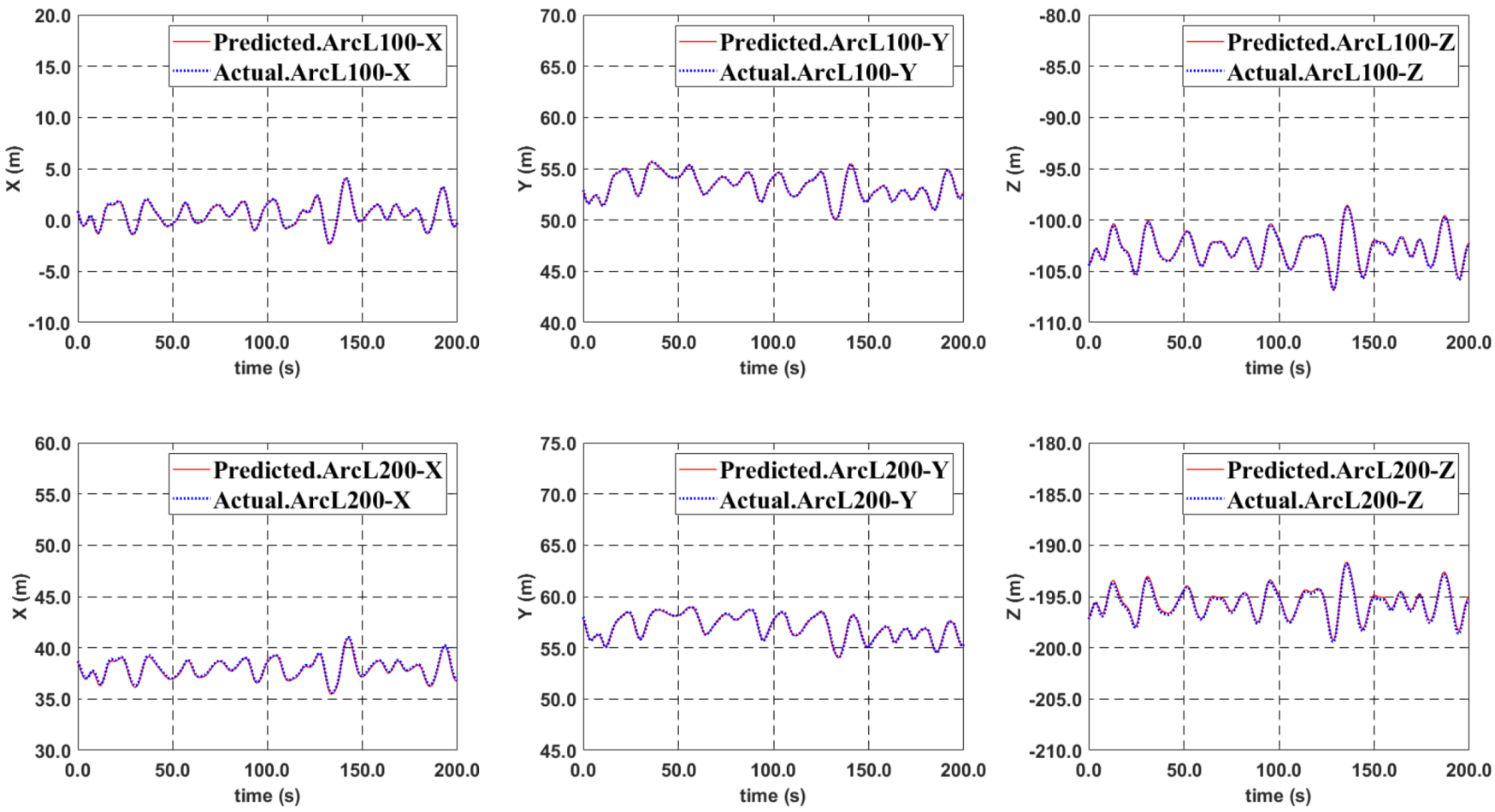
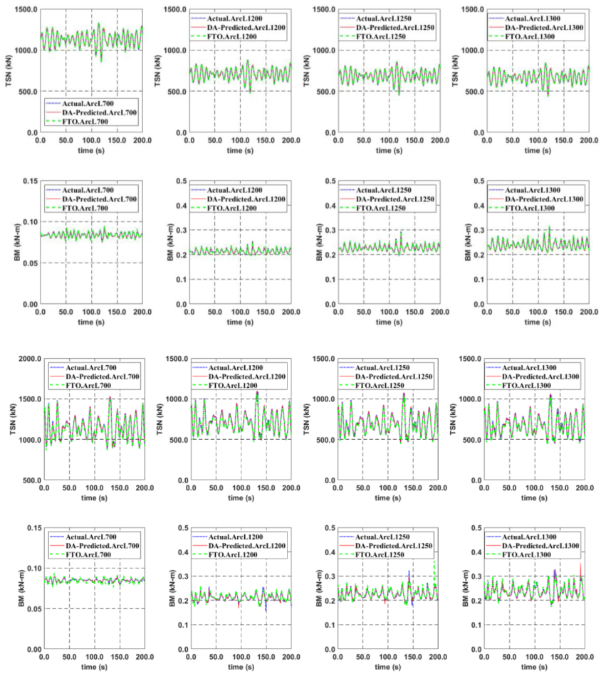
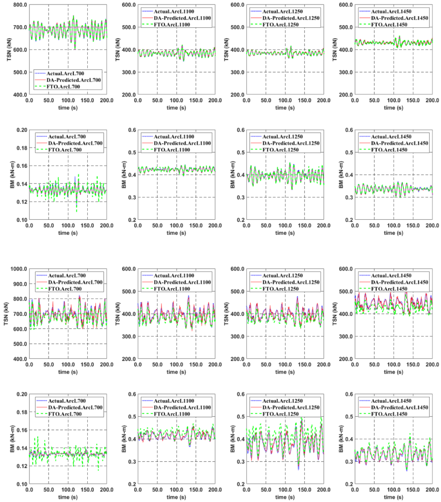
In the above section, the riser tracing algorithm using angle sensors was explained. As a FE simulator for line dynamics, we used a commercial program OrcaFlex. In this section, numerical results for two different approaches, the proposed DA method and the simpler FTO method, will be presented, and they will be compared with the actual values. The predicted node displacements, tensions, and bending moments at various riser locations will be compared with the corresponding actual values. As for environmental conditions, 1-yr and 100-yr storms with noncollinear wind-wave-current are considered as summarized in

Table 4. Environmental Conditions.

Type	Parameter	Unit	Operating (1-yr)	Extreme (100-yr)
Wave	Spectrum	(-)	JONSWAP	JONSWAP
	Gamma (Enhancement Parameter)	(-)	2.2	2.2
	Direction from North	(deg)	45	45
	Significant Wave Height (Hs)	(m)	3.5	8.7
	Peak Period (Tp)	(s)	10.3	17.2
Current	Surface Velocity (1/7 law is used)	(m/s)	0.3	1.0
	Direction from North	(deg)	90	90
Wind	Spectrum	(-)	API	API
	Mean Velocity at 10 m Elevation	(m/s)	20	34
	Direction from North	(deg)	60	60

. The wave, current, and wind headings are 45 deg, 90 deg, and 60 deg, respectively. This noncollinear environment is intentionally employed to trigger 3D riser dynamics. According to Equation (17), the current profile was inputted with given surface velocity (Figure 8). As an example floating system, OrcaFlex default FPSO with mooring (SPM) system is selected [32]. The FPSO dimension and specifications are tabulated in

Table 5. FPSO Dimension and Specification [32].

Length between Perpendiculars	Breadth	Draught	Mass	Ixx
m	m	m	ton	ton-m2
103	15.95	6.66	8800	249,000
Iyy	Izz	Xcg	Ycg	Zcg
ton-m2	ton-m2	m	m	m
5,830,000	5,830,000	2.53	0	−1.97

. Additionally, the mooring and riser coordinates and their arrangement are presented in

Table 6. Mooring Lines and Riser Coordinates and Lengths.

	Line No.	Fairlead Point			Anchor Point			Length
		X	Y	Z	X	Y	Z
		m	m	m	m	m	m	m
Mooring Lines	1	8.66	5.00	−7.50	679.03	563.97	−1000.0	1400.0
	2	7.07	7.07	−7.50	471.76	755.61	−1000.0	1400.0
	3	5.00	8.66	−7.50	233.28	869.29	−1000.0	1400.0
	4	−5.00	8.66	−7.50	−622.40	694.81	−1000.0	1400.0
	5	−7.07	7.07	−7.50	−761.90	547.30	−1000.0	1400.0
	6	−8.66	5.00	−7.50	−863.13	377.11	−1000.0	1400.0
	7	−8.66	−5.00	−7.50	−863.13	−377.11	−1000.0	1400.0
	8	−7.07	−7.07	−7.50	−761.90	−547.30	−1000.0	1400.0
	9	−5.00	−8.66	−7.50	−622.40	−694.81	−1000.0	1400.0
	10	5.00	−8.66	−7.50	233.28	−869.29	−1000.0	1400.0
	11	7.07	−7.07	−7.50	471.76	−755.61	−1000.0	1400.0
	12	8.66	−5.00	−7.50	679.03	−563.97	−1000.0	1400.0
SCR	[-]	0.00	0.00	−7.50	940.00	0.00	−1000.0	1500.0
SLWR	[-]	0.00	0.00	−7.50	890.00	0.00	−1000.0	1500.0

and Figure 9. The FPSO motions under 1-year and 100-year storms are plotted in Figure 10. The corresponding results for both SCR and SLWR are presented in the following.

$$\mathrm{V}={\mathrm{V}}_{\mathrm{sb}}+\left({\mathrm{V}}_{\mathrm{sf}}-{\mathrm{V}}_{\mathrm{sb}}\right)·{[\frac{\left(\mathrm{z}-{\mathrm{z}}_{\mathrm{sb}}\right)}{\left({\mathrm{z}}_{\mathrm{sf}}+{\mathrm{z}}_{\mathrm{sb}}\right)}]}^{\frac{1}{7}}$$

(17)

${\mathrm{V}}_{\mathrm{sb}},{\mathrm{V}}_{\mathrm{sf}}=\mathrm{current}\mathrm{velocity}\mathrm{at}\mathrm{seabed}\mathrm{and}\mathrm{surface}$${\mathrm{z}}_{\mathrm{sb}},{\mathrm{z}}_{\mathrm{sf}}=\mathrm{vertical}\mathrm{coordinate}\mathrm{of}\mathrm{seabed}\mathrm{and}\mathrm{surface}$

6. Numerical Results for Riser Structure Health Monitoring

6.1. SCR (Steel Catenary Riser)

First, the developed DA approach was applied to the SCR of FPSO. As previously explained, by using the quadratic interpolation function and curve length equation in 3D space, the node displacements can be traced progressively using the angle sensor information and top point measurement. Additionally, the tension can also be traced, as described in the previous section. Figure 11 and Figure 12 show that the suggested algorithm can actually trace the node displacements and tensions very well up to the target location at 200 m arclength (≈submergence depth) when the predicted values are compared with the actual values. The results are given for both 1-yr and 100-yr noncollinear storms to make sure that the schemes work for any sea conditions. Then, the FE riser-dynamics simulator was applied with the obtained movement and tension at the target point. Below the target point of 200 m submergence depth, the wave action is sufficiently attenuated, so wave inputs need not be included in the FE simulator. Instead, the wave effects are indirectly reflected through sensor signals and the tracing algorithm. Similarly, the effect of current above the target point is already indirectly included through the tracing algorithm. On the other hand, when the current penetrates deeper than 200 m, current below the target point needs to be included in the FE simulator. Then, the displacements, tensions, and bending moments can be obtained for any locations below the last sensor position (= target point) through the FE-simulator outputs in near real-time. The associated time lag is within a couple of seconds since the run time of the tracing algorithm and the FE simulator is an order of one second with a typical PC. The corresponding accuracies for tracing riser motions below the target point are presented additionally in Appendix A. The results show that the entire riser profile can be very well traced by using the present DA approach.

In the case of SCR, the dynamics near TDP (touch down point) is the most critical including the possibility of local dynamic buckling under the 100-yr storm [35,36]. Therefore, the tensions and bending moments at three locations (1200 m, 1250 m, and 1300 m) near the TDP are presented. One additional mid-length location (700 m) is also selected. In Figure 13, the comparisons of the time histories of tension and bending moment at four locations are shown. The predicted values by the suggested DA and simpler FTO approaches are compared with the actual values. Good agreements between the actual and DA-predicted values can be observed for both 1-yr and 100-yr storms. This means that the developed tracing algorithm and the subsequent FE simulator can capture the actual dynamic behaviors of the riser in near real-time. The figure also shows that even the simpler FTO approach roughly follows the actual values while the corresponding overall accuracy is diminished compared to the DA approach (see Appendix B). The errors of the FTO approach in the 100-yr storm are larger than those in the 1-yr storm since wave actions on the upper portion of the riser were neglected, i.e., the neglected wave effects of the former are expected to be larger than those of the latter. It should also be reminded that the current effect is not included in the FTO approach. The corresponding statistical characteristics, typical errors, and their comparisons are tabulated in Appendix B. From these results, it can be concluded that the present DA approach is reliable and accurate in tracing displacements, tensions, and bending moments along the entire length of the riser. The simpler FTO approach has larger errors but is still practically useful when high accuracy is not an important concern. The FTO’s error is particularly increased over the upper portion of the riser since direct wave action on riser is not included there.

6.2. SLWR (Steel Lazy Wave Riser)

Similarly, to demonstrate the performance of the developed DA-based riser monitoring capability, the same FPSO with different riser (SLWR) is employed here. As previously presented, both DA and FTO methods are used and compared for the same noncollinear 1-yr and 100-yr storms. The corresponding displacements, tensions, and bending moments at similar reference positions are presented. In the case of SLWR, the lazy wave zone is the most critical with high curvature, while the importance of the TDP is lessened [37].

The comparisons between the actual and predicted displacements and tensions up to the target point are presented in Figure 14 and Figure 15. Here, again, it is confirmed that the tracing algorithm can reproduce reasonably accurate node displacements and tensions up to the target location regardless of riser shape and sea state.

Next, as before, the FE simulator was run for the SLWR with the estimated movements and tensions at the target point. The corresponding tension and bending-moment results below the target point are presented in Figure 16. Since the lazy wave zone (= arc length 1200–1350 m) is the most critical region for SLWR system, three different locations (1100 m, 1250 m, and 1450 m) near the lazy wave zone and one additional middle part (700 m) are selected and compared. The corresponding comparisons of displacement snapshots are given in Appendix A, which shows that by using the proposed DA-based hybrid method, the predicted values agree well with the actual values. In the case of SLWR, the free-hanging portion of the riser is much longer than that of SCR, and thus the riser movements are more influenced by the wave and current. Therefore, the errors associated with the simpler approach FTO are generally larger than those in the SCR case, especially in the 100-yr storm (see Appendix B). The corresponding statistical characteristics and associated errors of the DA-based and FTO-based approaches are tabulated in Appendix B. The errors of the FTO method in bending moment on the upper portion of the SLWR are particularly pronounced in the 100-yr storm since the wave action is not considered in the upper portion.

Judging from the presented results for both SCR and SLWR, by attaching only several sensors on the top part of riser (free of battery replacement and data acquisition issues), riser structural health motoring over the entire length is possible regardless of riser type and ocean environmental condition. Furthermore, the proposed DA methodology does not have any restrictions regarding line shape and material properties so that it can be applied to any kind of line, such as umbilical, tendon, mooring line, and power cable. Thus, in Appendix C, another material sensitivity test (small bending stiffness and lightweight such as umbilical) was performed additionally.

Since real-time tensions and bending stresses can be monitored by the developed method, the continuous assessment of accumulated fatigue damage of lines is also possible [2,15], which is important for the extended-service-life estimation. So far, the demonstration of the performance of the developed methodology was based on numerical sensors, which is an ideal case that can read the actual angle values without any noise or error. In reality, sensor noises and errors may be involved. Authors’ another paper [16] showed that the developed algorithms were relatively robust against those typical mechanical-sensor noises/errors.

7. Conclusions

In this paper, a novel and cost-effective riser structural health monitoring methodology with a minimal number of sensors on the top portion of riser was developed to overcome various problems (power supply and data acquisition) associated with sensors (bi-axial inclinometers) at the deep portion of riser. The new approach was called the DA (dual algorithm) hybrid method since both the displacement tracing algorithm based on sensor signals and the FE simulator are simultaneously used. The displacement tracing algorithm traced the node displacement and tension up to the last sensor position, called the target point. Then, the inputted movement and tension of the target point were used for the FE simulator to obtain displacement, tension, and bending stress below the target point. This way, the real-time tracing of stresses along the entire riser can be reproduced.

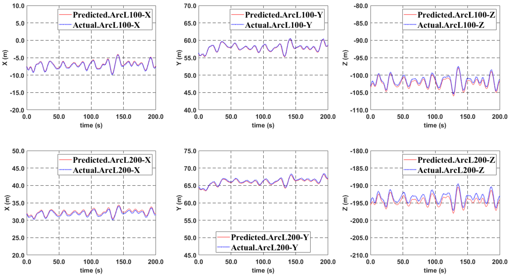
The developed DA-based hybrid method was validated by comparing the actually simulated riser dynamic behaviors with the reconstructed values by using the developed method. For that, a spread-moored FPSO system at 1000 m water depth with SCR or SLWR was employed with the assumption that angle sensors are positioned at the riser top portion, i.e., 0 m, 100 m, and 200 m arc lengths. Noncollinear wind-wave-current conditions representing 1-yr and 100-yr storms were used. It is confirmed that the developed DA method can reliably trace the real-time displacements, tensions, and bending stresses along the entire length of the riser.

As a simpler approach, forced top oscillation (FTO), which only uses riser top movement for running the FE simulator, was also introduced, and its performance was compared with that of DA. It was seen that the simpler method (FTO) could not accurately reproduce the dynamics of the upper portion of riser since real-time wave actions were ignored. Finally, it was also shown that the developed DA method was relatively robust against other kinds of lighter and more flexible lines, such as umbilical. Since the developed approach is generic regardless of line shape or material, it can also be applied to the real-time monitoring of flexible riser, mooring, and power cable.

8. Future Work

In present study, VIV (vortex-induced vibration) induced by current was not considered since fully straked risers were assumed. VIV for non-strake risers is important, which will be investigated in future studies. Moreover, validation of the suggested approach against real-experiment or field data will be conducted, and results will be presented/discussed in the sequel paper.

References

1. Chung, W.C.; Kang, H.Y.; Kim, M.H. Numerical Study on OPB/IPB Interlink Angle with Underwater Chain Stopper System. In Proceedings of the SNAME 24th Offshore Symposium, Houston, TX, USA, 20 February 2019. [Google Scholar]
2. Chung, W.; Kang, H.; Kim, M. Multi-scale approach for chain-mooring OPB-induced failure considering time-varying interlink bending stiffness and fairlead condition. Appl. Ocean Res. 2020, 98, 102128. [Google Scholar] [CrossRef]
3. Chung, W.C.; Kim, M. Effects of various fairlead-connection parameters on chain-mooring OPB-induced failure. Mar. Struct. 2021, 76, 102926. [Google Scholar] [CrossRef]
4. Andersen, M.; Berg, A.; Saevik, S. Development of an optical monitoring system for flexible risers. In Proceedings of the Offshore Technology Conference, Houston, TX, USA, 30 April–3 May 2001. [Google Scholar]
5. Kim, H.; Jin, C.; Kim, M.; Kim, K. Damage detection of bottom-set gillnet using Artificial Neural Network. Ocean. Eng. 2020, 208, 107423. [Google Scholar] [CrossRef]
6. Ziegler, L.; Muskulus, M. Lifetime extension of offshore wind monopiles: Assessment process and relevance of fatigue crack inspection. In Proceedings of the 12th EAWE PhD Seminar, DTU, Lyngby, Denmark, 25–27 May 2016. [Google Scholar]
7. Karayaka, M.; Ruf, W.; Natarajan, S. Steel catenary riser response characterization with on-line monitoring devices. In Proceedings of the International Conference on Offshore Mechanics and Arctic Engineering, Honolulu, HI, USA, 31 May–6 June 2009; pp. 687–698. [Google Scholar]
8. O’Donnell, D.; Srbinovsky, B.; Murphy, J.; Popovici, E.; Pakrashi, V. Sensor measurement strategies for monitoring offshore wind and wave energy devices. In Proceedings of the Journal of Physics: Conference Series, Ghent, Belgium, 24–26 August 2015; p. 012117. [Google Scholar]
9. Li, B.; Wang, H.; Shen, X.; Yan, Y.; Yang, F.; Hua, F. Deep-water riser fatigue monitoring systems based on acoustic telemetry. J. Ocean Univ. China 2014, 13, 951–956. [Google Scholar] [CrossRef]
10. McNeill, S.; Angehr, P.; Kluk, D.; Saruhashi, T.; Sawada, I.; Kyo, M.; Miyazaki, E.; Yamazaki, Y. A Method for Determining Quasi-Static and Dynamic Riser Inclination Using Collocated Accelerometers and Angular Rate Sensors. In Proceedings of the International Conference on Offshore Mechanics and Arctic Engineering, San Francisco, CA, USA, 8–14 June 2014; p. V06BT04A003. [Google Scholar]
11. Morikawa, S.; Camerini, C.S.; Braga, A.; Llerena, R.A. Real time continuous structural integrity monitoring of flexible risers with optical fiber sensors. In Proceedings of the Offshore Technology Conference, Houston, TX, USA, 3–6 May 2010. [Google Scholar]
12. Peng, R.; Zhi, Z. A state-of-the-art review on structural health monitoring of deepwater floating platform. Pac. Sci. Rev. A Nat. Sci. Eng. 2012, 14, 253–263. [Google Scholar]
13. Kim, H.-C.; Kim, M.-H.; Choe, D.-E. Structural health monitoring of towers and blades for floating offshore wind turbines using operational modal analysis and modal properties with numerical-sensor signals. Ocean Eng. 2019, 188, 106226. [Google Scholar] [CrossRef]
14. Chung, W.; Kang, H.; Kim, M.; Pestana, R.G. Riser Structural Health Monitoring with Numerical Sensors. In Proceedings of the 29th International Ocean and Polar Engineering Conference, Honolulu, HI, USA, 16–21 June 2019. [Google Scholar]
15. Chung, W.C.; Pestana, G.R.; Kim, M. Structural health monitoring for TLP-FOWT (floating offshore wind turbine) tendon using sensors. Appl. Ocean Res. 2021, 113, 102740. [Google Scholar] [CrossRef]
16. Chung, W.C.; Kim, M.; Jin, C. Real-time trace of riser profile and stress with numerical inclinometers. Ocean Eng. 2021, 234, 109292. [Google Scholar] [CrossRef]
17. Kim, H.; Jin, C.; Kim, M. Real-time estimation of riser’s deformed shape using inclinometers and Extended Kalman Filter. Mar. Struct. 2021, 77, 102933. [Google Scholar] [CrossRef]
18. Kwon, D.-S.; Jin, C.; Kim, M. Prediction of dynamic and structural responses of submerged floating tunnel using artificial neural network and minimum sensors. Ocean Eng. 2022, 244, 110402. [Google Scholar] [CrossRef]
19. Kwon, D.-S.; Jin, C.; Kim, M.; Koo, W. Mooring-failure monitoring of submerged floating tunnel using deep neural network. Appl. Sci. 2020, 10, 6591. [Google Scholar] [CrossRef]
20. Sengupta, B.; Ahmad, S. Reliability assessment of tension leg platform tethers under nonlinearly coupled loading. Reliab. Eng. Syst. Saf. 1996, 53, 47–60. [Google Scholar] [CrossRef]
21. Tonelli, D.; Luchetta, M.; Rossi, F.; Migliorino, P.; Zonta, D. Structural health monitoring based on acoustic emissions: Validation on a prestressed concrete bridge tested to failure. Sensors 2020, 20, 7272. [Google Scholar] [CrossRef]
22. Barshan, B. Fast processing techniques for accurate ultrasonic range measurements. Meas. Sci. Technol. 2000, 45, 45–50. [Google Scholar] [CrossRef]
23. Jarvis, A.J.C.; Cegla, F.B. Application of the distributed point source method to rough surface scattering and ultrasonic wall thickness measurement. J. Acoust. Soc. Am. 2012, 132, 1325–1335. [Google Scholar] [CrossRef]
24. Cegla, F.B.; Cawley, P.; Allin, J.; Davies, J. High-temperature (>500 °C) wall thickness monitoring using dry-coupled ultrasonic waveguide transducers. IEEE Trans. Ultrason. Ferroelectr. Freq. Control 2011, 58, 156–167. [Google Scholar] [CrossRef]
25. Kobayashi, M.; Jen, C.K.; Bussiere, J.F.; Wu, K.T. High-temperature integrated and flexible ultrasonic transducers for nondestructive testing. NDT E Int. 2009, 42, 157–161. [Google Scholar] [CrossRef] [Green Version]
26. Rao, B.P.C. Magnetic flux leakage technique: Basics. J. Nondestruct. Test. Eval. 2012, 11, 7–17. [Google Scholar]
27. Shi, Y.; Zhang, C.; Li, R.; Cai, M.; Jia, G. Theory and application of magnetic flux leakage pipeline detection. Sensors 2015, 15, 31036–31055. [Google Scholar] [CrossRef] [Green Version]
28. Jahangiri, V.; Mirab, H.; Fathi, R.; Ettefagh, M.M. TLP structural health monitoring based on vibration signal of energy harvesting system. Lat. Am. J. Solids Struct. 2016, 13, 897–915. [Google Scholar] [CrossRef] [Green Version]
29. Pipa, D.; Morikawa, S.; Pires, G.; Camerini, C.; Santos, J. Flexible riser monitoring using hybrid magnetic/optical strain gage techniques through RLS adaptive filtering. EURASIP J. Adv. Signal Process. 2010, 2010, 176203. [Google Scholar] [CrossRef] [Green Version]
30. Kim, H.-J.; Jang, B.-S.; Park, C.-K.; Bae, Y.H. Fatigue analysis of floating wind turbine support structure applying modified stress transfer function by artificial neural network. Ocean Eng. 2018, 149, 113–126. [Google Scholar] [CrossRef]
31. Kim, M.; Koo, B.; Mercier, R.; Ward, E. Vessel/mooring/riser coupled dynamic analysis of a turret-moored FPSO compared with OTRC experiment. Ocean Eng. 2005, 32, 1780–1802. [Google Scholar] [CrossRef]
32. Orcina. OrcaFlex Manual; Orcina Ltd.: Ulverston, UK, 2014. [Google Scholar]
33. Sparks, C. Fundamentals of Marine Riser Mechanics: Basic Principles and Simplified Analyses; PennWell Books, LLC: Tulsa, OK, USA, 2018. [Google Scholar]
34. Chung, W.C. Development of Offshore Structures (Mooring/Riser) Performance Assessment and Monitoring using Computer Simulations and Numerical Sensors. Ph.D. Thesis, Texas A&M University, College Station, TX, USA, 2021. [Google Scholar]
35. Eom, T.; Kim, M.; Bae, Y.; Cifuentes, C. Local dynamic buckling of FPSO steel catenary riser by coupled time-domain simulations. Ocean Syst. Eng 2014, 4, 215–241. [Google Scholar] [CrossRef]
36. Kim, S.; Kim, M.-H. Dynamic behaviors of conventional SCR and lazy-wave SCR for FPSOs in deepwater. Ocean Eng. 2015, 106, 396–414. [Google Scholar] [CrossRef]
37. Kim, S.; Kim, M.-H. Effects of geometric shape of LWSCR (lazy-wave steel catenary riser) on its global performance and structural behavior. Ocean Syst. Eng. 2018, 8, 247–279. [Google Scholar]
Figure 1. Scheme for the Derivation of Curved Line Length Equation in 3D.
Jmse 10 01994 g001
Figure 2. Configuration for Node Displacements and Discretized Bending Moment Tracing.
Jmse 10 01994 g002
Figure 3. Tension distribution estimation model.
Jmse 10 01994 g003
Figure 4. Bending moment estimation model.
Jmse 10 01994 g004
Figure 5. Scheme View (top) and Flowchart (bottom) of Dual-Algorithm Model for Riser Health Monitoring with Minimum Sensors.
Jmse 10 01994 g005
Figure 6. Schematic view of FPSO with SCR or SLWR, WD1000 (Arc Length = 1500 m).
Jmse 10 01994 g006
Figure 7. Comparison among Actual vs. Dual-Algorithm vs. Forced Top Oscillation of SCR and SLWR system, WD1000 (Arc Length = 1500 m).
Jmse 10 01994 g007
Figure 8. Current Profile, 1-yr and 100-yr Cases.
Jmse 10 01994 g008
Figure 9. Mooring and Riser (SCR) Arrangement.
Jmse 10 01994 g009
Figure 10. FPSO Motions, 1-yr Storm (Up) and 100-yr Storm (Down).
Jmse 10 01994 g010
Figure 11. Displacement Tracing up to Target Point (200 m Arclength), 1-yr Storm (Up) and 100-yr Storm (Down), WD1000, SCR, Sensor Interval = 100 m.
Jmse 10 01994 g011aJmse 10 01994 g011b
Figure 12. Tension Estimation up to Target Point, 1-yr Storm (Up) and 100-yr Storm (Down), WD1000, SCR, Sensor Interval = 100 m.
Jmse 10 01994 g012
Figure 13. Structural-Health Monitoring Performance Comparison Near Touch Down Zone (= Arclength 1150–1250 m) and Near Mid-Length (700 m) between DA and FTO Approaches: 1-yr Storm (Up) and 100-yr Storm (Down), WD1000, SCR, Sensors at 0 m, 100 m, and 200 m Arc Lengths Only.
Jmse 10 01994 g013
Figure 14. Displacement Tracing up to Target Point (200 m Arc length), 1-yr Storm (Up) and 100-yr Storm (Down), WD1000, SLWR, Sensor Interval = 100 m.
Jmse 10 01994 g014aJmse 10 01994 g014b
Figure 15. Tension Estimation up to Target Point, 1-yr Storm (Up) and 100-yr Storm (Down), WD1000, SLWR, Sensor Interval = 100 m.
Jmse 10 01994 g015
Figure 16. Structural-Health Monitoring Performance Near Touch Down Zone (= Arc Length 1200–1350 m) and Middle Part (700 m) by DA and FTO Approaches: 1-yr Storm (Up) and 100-yr Storm (Down), WD1000, SLWR, Sensors at 0 m, 100 m, and 200 m Arc Lengths Only.
Jmse 10 01994 g016