Marine Radar Oil Spill Extraction Based on Texture Features and BP Neural Network

Abstract

Marine oil spills are one of the major threats to marine ecological safety, and the rapid identification of oil films is of great significance to the emergency response. Marine radar can provide data for marine oil spill detection; however, to date, it has not been commonly reported. Traditional marine radar oil spill research is mostly based on grayscale segmentation, and its accuracy depends entirely on the selection of the threshold. With the development of algorithm technology, marine radar oil spill extraction has gradually come to focus on artificial intelligence, and the study of oil spills based on machine learning has begun to develop. Based on X-band marine radar images collected from the Dalian 716 incident, this study used image texture features, the BP neural network classifier, and threshold segmentation for oil spill extraction. Firstly, the original image was pre-processed, to eliminate co-channel interference noise. Secondly, texture features were extracted and analyzed by the gray-level co-occurrence matrix (GLCM) and principal component analysis (PCA); then, the BP neural work was used to obtain the effective wave region. Finally, threshold segmentation was performed, to extract the marine oil slicks. The constructed BP neural network could achieve 93.75% classification accuracy, with the oil film remaining intact and the segmentation range being small; the extraction results were almost free of false positive targets, and the actual area of the oil film was calculated to be 42,629.12 m². The method proposed in this paper can provide a reference for real-time monitoring of oil spill incidents.

1. Introduction

Oil spills cause damage to the marine ecosystem. Timely monitoring and identification of oil slicks after an oil spill is of great importance in mitigating hazards [1]. Marine radar is a mobile, portable, economical, high-spatial and temporal-resolution oil spill monitoring device that can be easily mounted on shore and ship bases [2]. After the first US experiments using marine radar to observe oil spills in the Gulf of California, research on marine radar oil spill monitoring began to increase. Countries such as the Netherlands, Norway, and Russia carried out several research studies on the detection and tracking of oil spills [3,4], which evaluated marine radar oil spill monitoring capability.

Since Dalian Maritime University conducted an oil spill monitoring task using marine radar in the Bohai Sea, and obtained radar images by digital processing, most studies have been carried out with quantified radar images [5]. Wang designed a marine radar oil spill monitoring system using a banalization algorithm, and the image processing effect was completely accurate in identifying oil films [6]. Zhu et al. proposed a power attenuation correction method, to solve the problem of uneven resolution and echo intensity distribution, and adapted Otsu thresholding segmentation to detect oil spills from different ocean backgrounds [7]. Liu et al. employed a power fitting method of radar echo, to detect oil spills on sampled X-band marine radar images, using a mean filter, the Otsu method, and connected component analysis to extract oil spills [8]. Xu et al. adapted the improved local adaptive thresholding method to segment the oil spills [9]. The accuracy of direct threshold methods for extracting oil films depends on the image pre-processing effect and the complexity of the oil spill: these methods cannot distinguish between oil films and oil-like films. With further research, scholars have introduced texture features and image classification algorithms. Liu et al. used the texture analysis method to determine the oil film area, based on marine radar images, and achieved the accurate extraction of oil film through a threshold segmentation algorithm [10]. Meanwhile, a texture index calculator, based on four texture features of the GLCM, was proposed, and machine learning methods such as the support vector machine (SVM), K-Nearest Neighbor (K-NN), linear discriminant analysis (LDA), and integrated learning (EL) were used to extract the coarse oil spill area indicated by the texture index. Finally, the oil spill area was finely measured, using adaptive thresholding [11]. Li et al. used GLCM to obtain local window radar image texture features, selected one texture feature as an input feature of the SVM classifier, to classify local window images, and, finally, applied FCM to accurately extract oil film [12]. Xu et al. combined LBP texture features and the K-means algorithm to propose an offshore oil detection method with threshold segmentation, which can automatically detect oil spills with shipboard radar images [13]. These methods are intelligent, and have improved oil spill detection efficiency and accuracy.

Marine radar-based final extraction of oil film has never been achieved without threshold segmentation, and this paper is no exception. We used X-band oil spill marine radar images as the basic data; we built a BP neural network classifier, based on texture features, and we applied sliding window threshold segmentation to extract the oil films. The method in this paper provides technical support for future maritime radar oil spill research, and could lay the foundation for emergency responses to oil spill incidents.

2. Materials and Methods

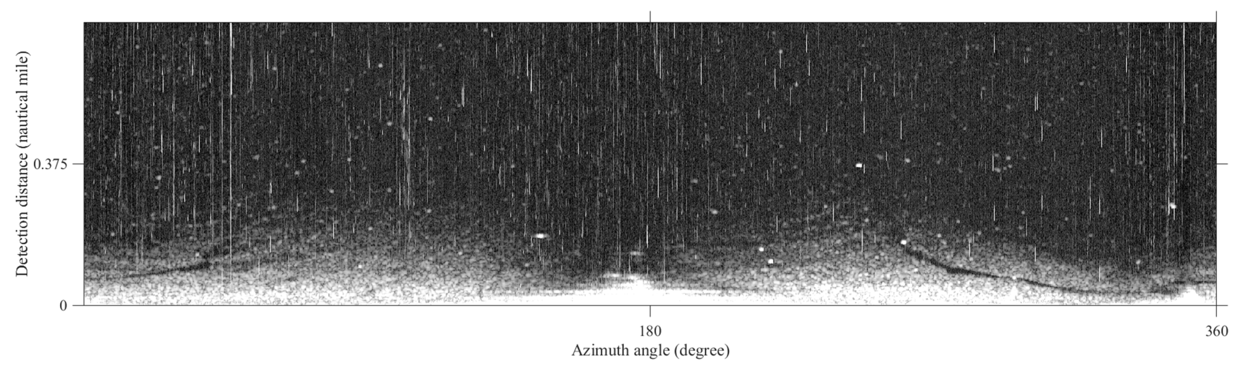
2.1. Experimental Data

The original datum of this paper was an X-band marine radar image, with the vertical direction indicating the detection distance, and the horizontal direction indicating the azimuth angle. The image size was 512 × 2048 pixels, and the image resolution was 2.71 m, as shown in Figure 1. It was acquired by the SPX card of the Sperry Marine radar system during the Dalian 716 oil pipeline explosion incident, at 23:19 on 21 July 2010: the sea surface wind speed was 6.5 m/s at that time, which was adequate for oil spill detection, and the weather was rain-free. The parameters of the Sperry Marine radar system are listed in

Table 1. The parameters of the Sperry Marine radar system.

Parameter	Value
Band	X-band
Detection distance	0.5/0.75/1.5/3/6/12/24 NMs
Angle resolution	0.1°
Antenna type	Waveguide split antenna
Polarization mode	Horizontal
Horizontal detection angle Vertical detection angle	360° ± 10°
Rotation speed	28–45 revolutions/min
Length of antenna	8 ft
Pulse recurrence frequency	3000 Hz/800 Hz/785 Hz
Pulse width	50 n/ns/ns

.

2.2. Image Preprocess

Due to the co-channel interference caused to the radar receiver when the noise signal was emitted at the same frequency as the useful signal, there were many bright lines on the original image. In order not to affect oil spill detection, noise reduction processing was required, to eliminate the co-channel interference noise. The image was first convolved laterally, to smooth out the co-channel interference noise; then, the Otsu algorithm was applied to the vertical line detection (Figure 2a); finally, linear interpolation was performed, to obtain the noise-reduced image (Figure 2b). The noise-reduced image was used for subsequent experiments in this paper.

2.3. Methods

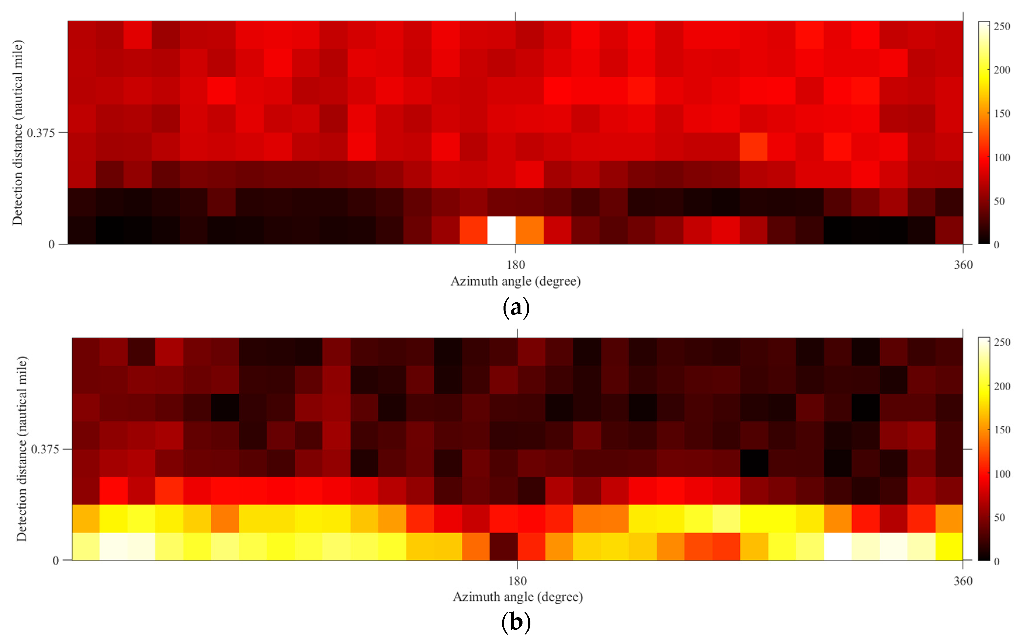
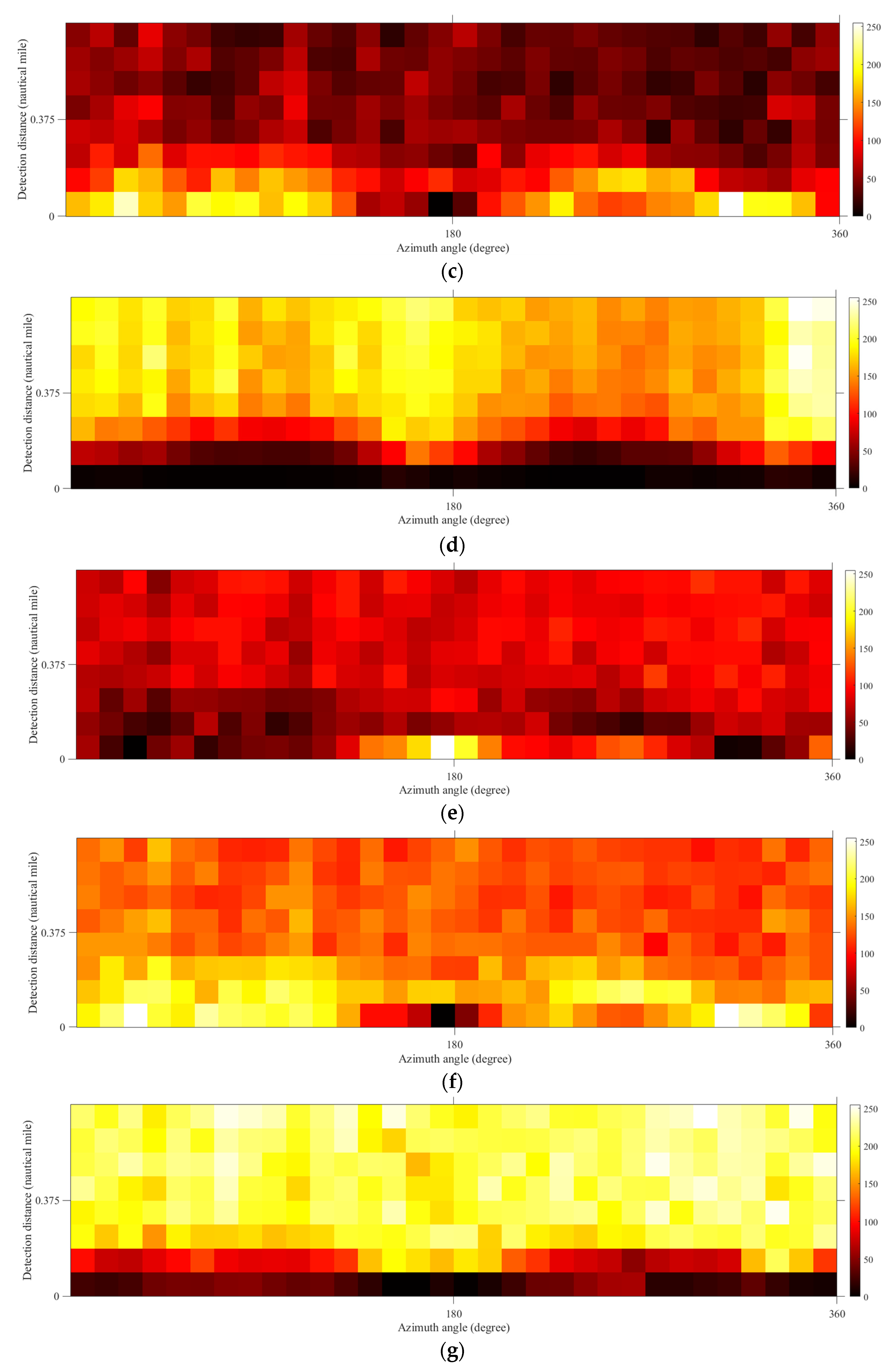
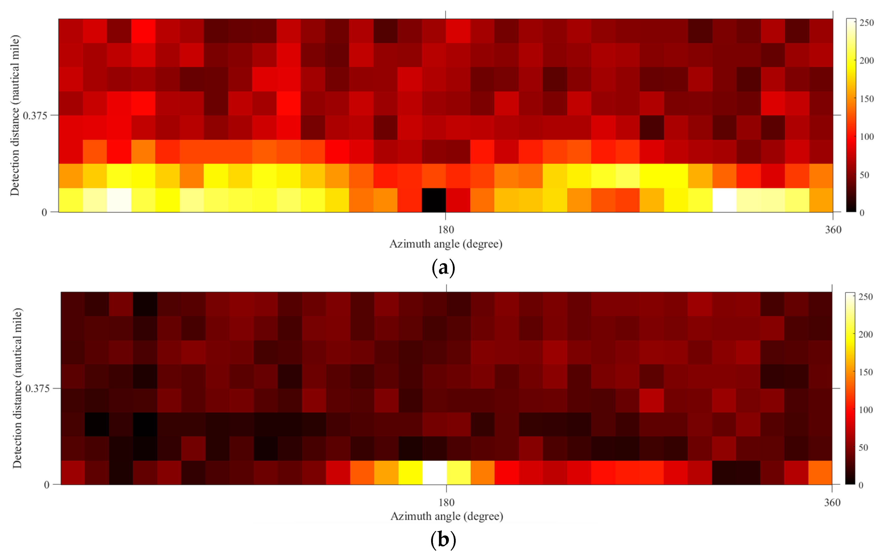
2.3.1. Image Texture Features

Because single-band radar images can only reflect differences in grayscale information, this paper introduced texture features to complement oil spill target identification. Haralick [14] et al. proposed the extraction of image texture features based on the GLCM, which is a common method of describing texture by studying the spatial correlation properties of grayscale: it simply refers to the probability of two image pixels (i, j) with distance d, direction θ, and grayscale values for i and j, respectively. The GLCM can be repressed as [15]:

$$P_{ij}=\frac{P\left(i,j,d,\theta \right)}{{{\displaystyle \sum }}_{i,j}P\left(i,j,d,\theta \right)}$$

(1)

A total of 14 texture features can calculated from GLCM [16]; the common texture feature expressions are shown in

Table 2. Expressions for texture features.

Texture Feature	Formula
Angular second moment	$f_{ASM}$$={\displaystyle \sum }_{i=0}^M{\displaystyle \sum }_{j=0}^{N}p{\left(i,j,d,\theta \right)}^2$
Entropy	$f_{ENT}$$=-{\displaystyle \sum }_{i=0}^M{\displaystyle \sum }_{j=0}^{N}p\left(i,j,d,\theta \right)logp\left(i,j,d,\theta \right)$
Contrast	$f_{CON}$$={\displaystyle \sum }_{i=0}^M{\displaystyle \sum }_{j=0}^N{\left(i-j\right)}^{2}p\left(i,j,d,\theta \right)$
Mean	$f_{MEAN}$$={\displaystyle \sum }_{i=0}^M{\displaystyle \sum }_{j=0}^{N}i\ast p\left(i,j,d,\theta \right)$
Homogeneity	$f_{HOM}$$={\displaystyle \sum }_{i=0}^M{\displaystyle \sum }_{j=0}^N\frac{p\left(i,j,d,\theta \right)}{1+{\left(i-j\right)}^2}$
Dissimilarity	$f_{DIS}$$={\displaystyle \sum }_{i=0}^M{\displaystyle \sum }_{j=0}^N\left|i-j\right|p\left(i,j,d,\theta \right)$
Correlation	$f_{COR}$$={\displaystyle \sum }_{i=0}^M{\displaystyle \sum }_{j=0}^N\frac{\left(i-\mu \right)\left(j-\mu \right)p\left(i,j,d,\theta \right)}{{\sigma }^2}$
Variance	$f_{var}$$={\displaystyle \sum }_{i=0}^M{\displaystyle \sum }_{j=0}^N{\left(i-\mu \right)}^{2}p\left(i,j,d,\theta \right)$

.

2.3.2. PCA

PCA is the process of turning multiple variables into fewer variables, through a certain linear combination. After dimensionality reduction, it is possible to retain most of the information from the original data, thus making the data easier to process. PCA’s main processes are detailed below [17].

Assume a sample data with n indicators $X_1$, $X_2$, …, $X_n$ denoting the individual characteristics of each object, with N samples, which can be expressed as an N × n matrix, that is $X={\left(X_{ij}\right)}_{N\times n}$; $i$ = 0, 1, 2, …, N, $j$ = 0, 1, 2, …, n.

The raw data are normalized to obtain the normalization matrix Y:

$$y_{ij}=\frac{x_{ij-}{\overline{x}}_j}{s_j};i=0,1,\dots ,N,j=0,1,\dots ,n$$

(2)

where ${\overline{x}}_j$ and $s_j$ are the mean and variance, respectively, of the indicator variable $X_j$.

• Calculate the correlation coefficient matrix for the standard variables:

  $$R=E\left(Y{Y}^T\right)$$

  (3)
• Calculate the eigenvalues ${\gamma }_1$, ${\gamma }_2$, …$,{\gamma }_n$ of the correlation coefficient matrix R and the corresponding eigenvectors $q_1$, $q_2$, …, $q_n$. Convert the normalized indicators into n principal components.
• The number of principal components is determined by calculating the contribution of the principal components. The contribution is expressed as:

  $$C=\frac{{\gamma }_i}{{{\displaystyle \sum }}_{i=1}^n{\gamma }_i}$$

  (4)

2.3.3. BP Neural Network

As the gray values of the experimental image outside the 0.375 nm range were similar to the oil film on the sea, there was a potential for large errors if the threshold segmentation was applied directly; therefore, we adapted the BP neural network to remove the distant sea area, and obtained the valid wave area before segmentation. The BP neural network is a multi-layer forward-type neural network that uses the gradient descent method to calculate the minimum value of the objective function, with the signal propagating forward, and the error propagating backward [18]. The network generally consists of an input layer, a hidden layer, and an output layer: each layer can contain multiple neurons, and any neuron in each layer is connected to all the neurons in the next layer, with no connection between the neurons in the layer [19]. The training process of the BP neural network [20] is shown in Figure 3.

Calculate the output layer:

$${\widehat{y}}_k={{\displaystyle \sum }}_{j=1}^l{h}_j{w}_{jk}-b_k,k=1,2,3,\dots ,m.$$

(5)

Calculate the hidden layer:

$$h_j=f\left({{\displaystyle \sum }}_{i=1}^n{w}_{ij}{x}_i-a_j\right),j=1,2,3,\dots ,l.$$

(6)

Calculate the error:

$$e_k=y_k-{\widehat{y}}_k$$

(7)

2.3.4. Construction of an Oil Film Extraction Method Based on Texture Features and the BP Neural Network

The BP neural network classifier (Figure 4), based on texture features and adaptive threshold segmentation, was constructed in combination with the above ideas, to extract oil films from the sea. The main processes are listed below:

• The image was sliced, to obtain a local window of the image;
• Each texture feature value was calculated; PCA was conducted for texture features;
• A BP neural network classifier was built on a certain number of training samples; based on the texture features, a neural network was constructed to obtain the valid oil spill region; finally, the accuracy was evaluated;
• Adaptive threshold segmentation was applied to the effective wave area, to extract the oil films.

3. Results

3.1. Sample Selection

In this paper, we chose three radar images (23:19 on 21 July 2010, 23:20 on 21 July 2010, and 23:21 on 21 July 2010) as the sample data, using the same slice processing to obtain 768 images of size 64 × 64 pixels, and labeling the background seawater and the valid wave regions for these images separately, as shown in Figure 5. Finally, 768 training samples were selected, of which 604 were background seawater, and 164 were valid wave regions.

3.2. Texture Features Extraction

The GLCM texture features extraction required consideration of step size, gray quantization level, orientation, and sliding window size. In order to accurately portray the relationship between adjacent image pixels, the step size d = 1 was chosen. In order to reduce the number of operations, 16 was used as the gray quantization level. Considering that the difference between the texture features of the four directions was not obvious, the average value was used as the final texture feature. As the texture features of the image slice were calculated, the sliding window size in this paper was the image slice size, which was 64 × 64. The texture features of the training and experimental data were calculated by the formula in Table 1. The results of the experimental image texture feature visualization are shown in Figure 6.

3.3. The PCA for Texture Features

As can be seen from the visualization results in Figure 6, different texture features reflected the difference between background seawater and the effective wave area, but with different intensities; therefore, in the selection of the texture features, dimensionality reduction was used, to determine the covariates that reflected the overall characteristics of the eight types of texture features.

In this study, we performed PCA of the image texture features, with the help of SPSS software, to obtain new principal components. The KMO test value of the experimental results was 0.704, and Bartlett’s spherical test was less than 0.05, indicating that the variables were not independent of each other, and were suitable for principal component analysis.

Table 3. Eigenvalues and contribution of principal components.

Principal Components	Eigenvalue	Variance Contribution Rate (%)	Cumulative Variance Contribution Rate (%)
1	5.782	72.277	72.277
2	1.650	20.625	92.902
3	0.303	3.789	96.690
4	0.144	1.800	98.490
5	0.06	0.751	99.241
6	0.049	0.607	99.848
7	0.011	0.138	99.986
8	0.001	0.014	100

shows the eigenvalues and contribution rates of each principal component. According to the theory of selecting principal components, the principal components with eigenvalues greater than 1, or cumulative variance contribution greater than 85%, were generally taken [21]. The first two principal components (PC) were selected, which explained 92.90% of the information of the original variables, and the loadings of the principal component factors were calculated, to characterize the original eight features into two principal components by linear combination.

The first principal component (y1) was expressed as:

y1 = −0.371x1 + 0.406x2 + 0.391x3 − 0.341x4 − 0.263x5 + 0.366x6 − 0.372x7 + 0.295x8

(8)

The second principal component (y2) was expressed as:

y2 = 0.281x1 + 0.1x2 − 0.037x3 − 0.308x4 + 0.595x5 − 0.357x6 − 0.312x7 + 0.487x8

(9)

where x1, x2, x3, …, x8 were texture feature energy, entropy, contrast, mean, homogeneity, dissimilarity, correlation, and variance.

PCA was used here to downscale the eight texture features to obtain the first and second principal components, which formed two new features (PC1 and PC2) to represent the overall characteristics of the texture features (Figure 6). PC1 and PC2 here were used to denote the image features, as shown in Figure 7.

3.4. BP Neural Network Training

When building a BP neural network, the number of nodes in the input layer, the hidden layer, and the output layer, as well as the transfer function, need to be defined. The output and input layer nodes are generally determined according to the research requirements, and the number of nodes in the hidden layer can be expressed according to the empirical formula:

$$L=\sqrt{n+m}+\mathrm{a}$$

(10)

where n is the number of nodes in the input layer, m is the number of nodes in the output layer, and “a” takes values between 1 and 10. Due to the randomness of the BP neural network weights and thresholds, resulting in different training results each time, the number of nodes in the hidden layer in this paper was obtained after repeated trials on the Matlab platform.

The BP neural network transfer functions are commonly known as logsig, tagsig, and purelin. The logsig is logarithmic sigmoid transfer function, expressed as:

$$logsig\left(n\right)=\frac{1}{1+\exp \left(n\right)}$$

(11)

The tagsig is symmetric sigmoid transfer function, expressed as:

$$tansig\left(n\right)=\frac{2}{1+\exp \left(-2n\right)}-1$$

(12)

The purelin is linear transfer function, expressed as:

$$y=n$$

(13)

In this experiment, we selected the network structure with two hidden layers, and the number of nodes in the hidden layer was 10. The number of nodes in the input layer was the two features (PC1 and PC2), to differentiate background seawater and the valid wave region; the number of nodes in the output layer was set to 2. The transfer function from the input layer to the hidden layer was logsig (formula (11)), and the transfer function from the hidden layer to the input layer was purelin (formula (13)). For the loss function, we used the mean squared error (mse) caculation, with the number of iterations set to 500; the result of the BP neural network classification is shown in Figure 8.

4. Discussion

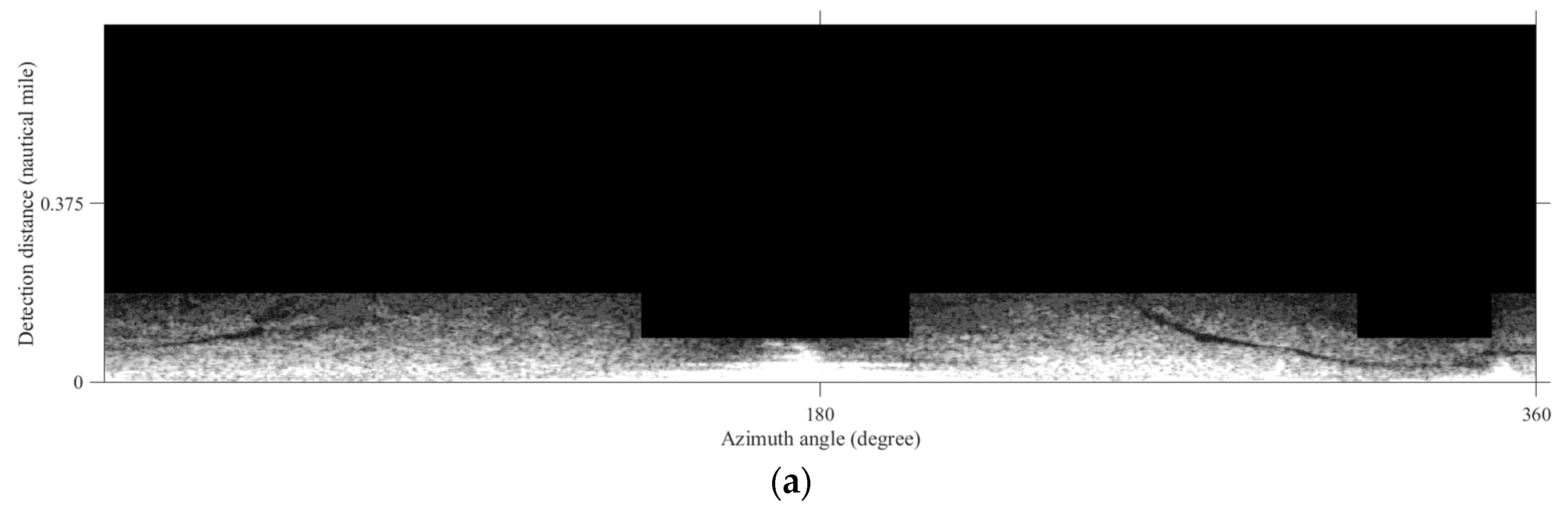
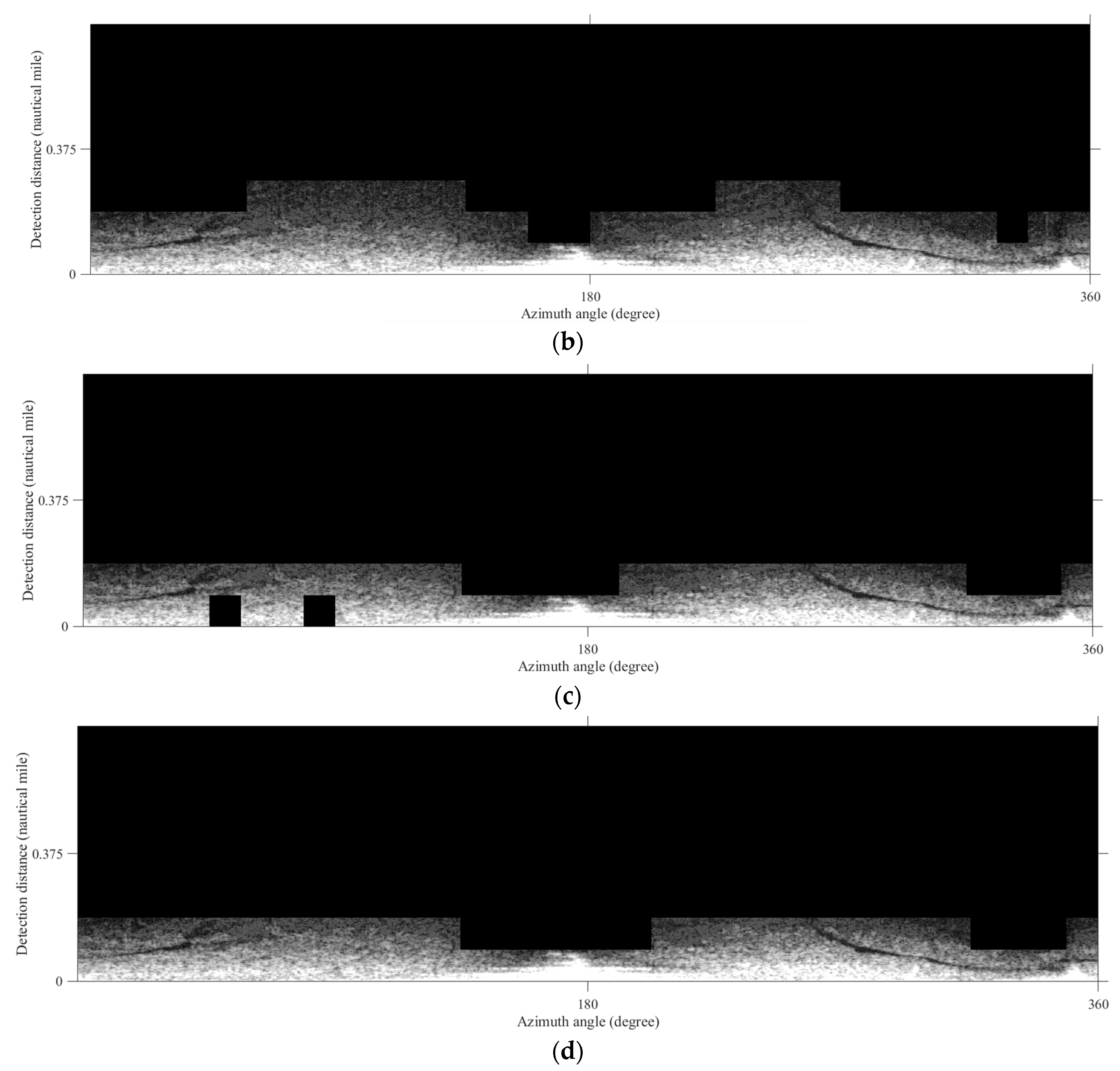
4.1. The Valid Wave Region Extraction

To verify the effectiveness of our experiment, the Decision Tree (DT), the K-Nearest Neighbor (K-NN), and the Random Forest (RF) classifiers were compared with the proposed method. The classification results are shown in Figure 9, the compute time and classification accuracy are displayed in

Table 4. Comparison of computing time and classification accuracy.

Classifier	Compute Time (s)	Classification Accuracy (%)
BP neural network	1.72	93.75
DT	1.12	92.97
K-NN	0.78	99.60
RF	2.27	93.75

. In terms of computing time and classification accuracy, K-NN worked best. Although the DT classifier outperformed the BP neural network and RF in terms of computing time, it was the worst in terms of classification accuracy. The BP neural network and RF had the same classification accuracy, but there was still a slight difference in classification time. From the extraction effect, four classification methods could ensure the integrity of the oil slicks, because the classification results of the RF and BP neural network classifiers were the same; the K-NN, DT, and BP neural network results were selected for the oil film segmentation.

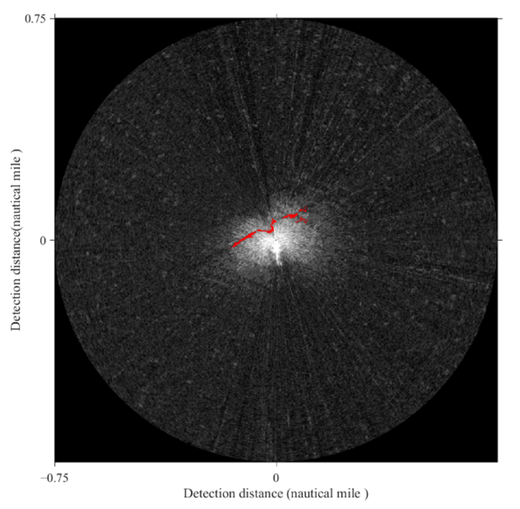
4.2. Adaptive Threshold Segmentation

The Sauvola algorithm was used to segment the valid wave regions, with a sliding window size of 72 × 72 pixels and an initial threshold k of 0.65. The segmentation results are shown in Figure 10. Due to the similar grayscale value and texture features of the oil film targets, the ship wake flow was mistakenly split out, and needed to be removed. The small spots were the noises created in the threshold segmentation process: they were deleted by setting the area threshold at “100”. The final oil film extraction results are shown in Figure 11; the estimated actual areas of the oil spill were obtained by counting pixels (

Table 5. Oil spills area.

Method	Pixels	Areas
BP Neural Network	5792	42,629.12
Decision tree	4557	33,539.52
K-NN	5975	43,976

). Compared with K-NN, it can be concluded that, under the condition of ensuring the integrity of the oil film, if the valid wave area was large, the oil films did not exist in the valid wave area: this may have caused errors in the segmentation process. Although K-NN performed better than the BP neural network in the extraction accuracy of the effective wave area, the oil film identification range became larger, and the probability of false positive targets increased during the segmentation; therefore, if the valid wave area could be reduced in size while ensuring the integrity of the oil film, the accuracy of the oil films split would be ensured. From this perspective, the method proposed here was superior to KNN, which produced the probability of incorrect segmentation. Compared with the BP neural network and K-NN, the DT extraction results had some oil films missing. In terms of the estimated actual area of the oil spill, the K-NN extracted area was large, due to the presence of false positive targets that were not completely removed, and the DT extracted area was small, due to the presence of some oil spill areas that were difficult to identify; therefore, the BP neural network classification was proposed for our method.

In practice, wave information monitoring by marine radar is carried out in the polar coordinate system, so the result of oil film identification in Cartesian coordinates needed to be converted, to obtain the final oil film identification result (Figure 12).

5. Conclusions

In this paper, the image texture features were extracted based on GLCM, selected by dimensionality reduction, and were linearly combined as the input features of the new feature quantity classifier; the BP neural network was constructed to classify the effective wave region; finally, the oil film was extracted using threshold segmentation. The effectiveness of the BP neural network classifier in this study was verified by comparing it with the traditional classifiers Decision Tree (DT), K-Nearest Neighbor (K-NN), and Random Forest (RF), based on training samples. From the classification results, the four methods did not differ greatly in terms of computing time and classification accuracy, which may have been related to the limited number of training and test samples. Future research could try to reduce the size of the classification image, or to increase the sample data, to solve this problem. In the oil spill extraction, the proposed method reduced the threshold segmentation range and the segmentation error, as well as ensuring classification accuracy. However, as the identification of ship wake flows relies on a priori knowledge and manual rejection, our method has not yet achieved fully automated intelligent oil spill identification. Future research needs to focus on how to distinguish oil films from oil-like films, such as ship wake flows, on radar images, as well as optimizing oil film identification and extraction algorithms. Nevertheless, this paper provides a method for maritime radar oil spill extraction research, which could play a role in oil spill incidents, and could provide assurance for marine accident emergency response.

References

1. Zhu, G.R.; Xie, Z.L.; Xu, H.L.; Wang, L.; Zhang, L.G.; Ma, N.; Cheng, J.X. Oil Spill Environmental Risk Assessment and Mapping in Coastal China Using Automatic Identification System (AIS) Data. Sustainability 2022, 14, 5327. [Google Scholar] [CrossRef]
2. Fingas, M.; Brown, C.E. A Review of Oil Spill Remote Sensing. Sensors 2018, 18, 91. [Google Scholar] [CrossRef] [PubMed] [Green Version]
3. Atanassov, V.; Mladenov, L.; Rangelov, R.; Savchenko, A. Observation of Oil Slicks on the Sea Surface by Using Marine Navigation Radar. In Proceedings of the Remote Sensing Conference: Global Monitoring for Earth Management, Espoo, Finland, 3–6 June 1991. [Google Scholar]
4. Tennyson, E.J. Shipboard Navigational Radar as an Oil Spill Tracking Tool. Int. Oil Spill Conf. Proc. 1989, 1989, 119–121. [Google Scholar] [CrossRef]
5. Feng, H.Y. Research on Wave and Oil Spill Information Extraction Method Based on Marine Radar; Dalian Maritime University: Dalian, China, 2015. [Google Scholar]
6. Wang, Z.Y. Research into Methods and Techniques for Monitoring Oil Spills on the Sea Surface by Marine Radar; Dalian Maritime University: Dalian, China, 2011. [Google Scholar]
7. Zhu, X.Y.; Li, Y.; Feng, H.Y.; Liu, B.X.; Xu, J. Oil spill detection method using X-band marine radar imager. J. Appl. Remote Sens. 2015, 9, 095985. [Google Scholar] [CrossRef]
8. Liu, P.; Zhao, Y.C.; Liu, B.X.; Li, Y.; Chen, P. Oil spill extraction from X-band marine radar images by power fitting of radar echoes. Remote Sens. Lett. 2021, 12, 345–352. [Google Scholar] [CrossRef]
9. Xu, J.; Cui, C.; Feng, H.Y.; You, D.M.; Wang, H.X. Marine Radar Oil-Spill Monitoring through Local Adaptive Thresholding. Environ. Forensics 2019, 20, 196–209. [Google Scholar] [CrossRef]
10. Liu, P.; Li, Y.; Xu, J.; Wang, T. Oil spill extraction by X-band marine radar using texture analysis and adaptive thresholding. Remote Sens. Lett. 2019, 10, 583–589. [Google Scholar] [CrossRef]
11. Liu, P.; Li, Y.; Liu, B.X.; Chen, P.; Xu, J. Semi-Automatic Oil Spill Detection on X-Band Marine Radar Images Using Texture Analysis, Machine Learning, and Adaptive Thresholding. Remote Sens. 2019, 11, 756. [Google Scholar] [CrossRef] [Green Version]
12. Li, B.; Xu, J.; Pan, X.X.; Ma, L.; Zhao, Z.Q. Marine Oil Spill Detection with X-Band Shipborne Radar Using GLCM, SVM and FCM. Remote Sens. 2022, 14, 3715. [Google Scholar] [CrossRef]
13. Xu, J.; Pan, X.X.; Jia, B.Z.; Wu, X.R.; Liu, P.; Li, B. Oil Spill Detection Using LBP Feature and K-means Clustering in Shipborne Radar Image. J. Mar. Sci. Eng. 2021, 9, 65. [Google Scholar] [CrossRef]
14. Haralick, S.; Robert, M.; Sternberg, R.; Zhuang, X.H. Image Analysis Using Mathematical Morphology. IEEE Trans. Pattern Anal. Mach. Intell. 1987, PAMI–9, 532–550. [Google Scholar] [CrossRef] [PubMed]
15. Benco, M.; Hudec, R.; Kamencay, P.; Zachariasova, M.; Matuska, S. An Advanced Approach to Extraction of Colour Texture Features Based on GLCM. Int. J. Adv. Robot. Syst. 2014, 11, 104. [Google Scholar] [CrossRef]
16. Zhao, Y.; Zhang, Z.P.; Zhu, H.L.; Ren, J.H. Quantitative Response of Gray-Level Co-Occurrence Matrix Texture Features to the Salinity of Cracked Soda Saline-Alkali Soil. Int. J. Environ. Res. Public Health 2022, 19, 6556. [Google Scholar] [CrossRef] [PubMed]
17. Booker, N.K.; Knights, P.; Gates, J.D.; Richard, C. Applying principal component analysis (PCA) to the selection of forensic analysis methodologies. Eng. Fail. Anal. 2022, 132, 105937. [Google Scholar] [CrossRef]
18. Ding, S.F.; Jia, W.K.; Su, C.Y.; Zhang, L.W.; Liu, L.L. Research of neural network algorithm based on factor analysis and cluster analysis. Neural Comput. Appl. 2011, 20, 297–302. [Google Scholar] [CrossRef]
19. Zhang, L.; Wang, F.L.; Sun, T.; Xu, B. A constrained optimization method based on BP neural network. Neural Comput. Appl. 2018, 29, 413–442. [Google Scholar] [CrossRef]
20. Han, W.; Nan, L.B.; Su, M.; Li, R.N.; Zhang, X.J. Research on the Prediction Method of Centrifugal Pump Performance Based on a Double Hidden Layer BP Neural Network. Energies 2019, 12, 2709. [Google Scholar] [CrossRef] [Green Version]
21. Marukatat, S. Tutorial on PCA and approximate PCA and approximate kernel PCA. Artif. Intell. Rev. 2022, 55, 1–33. [Google Scholar] [CrossRef]
Figure 1. The original radar image.
Jmse 10 01904 g001
Figure 2. Image preprocess: (a) the noises were segmented; (b) the noise-reduced image.
Jmse 10 01904 g002
Figure 3. The training process of BP Neural Network.
Jmse 10 01904 g003
Figure 4. Construction of a BP neural network classifier based on texture features.
Jmse 10 01904 g004
Figure 5. Training data: (ac) were different radar images concluding oil spills.
Jmse 10 01904 g005aJmse 10 01904 g005b
Figure 6. Experimental image texture features: (a) energy; (b) entropy; (c) contrast; (d) mean; (e) homogeneity; (f) dissimilarity; (g) correlation; (h) variance.
Jmse 10 01904 g006aJmse 10 01904 g006bJmse 10 01904 g006c
Figure 7. The visualizations of PC1 and PC2: (a) PC1; (b) PC2.
Jmse 10 01904 g007
Figure 8. The result of BP neural network training.
Jmse 10 01904 g008
Figure 9. The valid wave region: (a) BP neural network; (b) K-Nearest Neighbor; (c) Decision Tree; (d) Random Forest.
Jmse 10 01904 g009aJmse 10 01904 g009b
Figure 10. The results of Sauvola segmentation: (a) BP neural network; (b) K-Nearest Neighbor; (c) Decision Tree.
Jmse 10 01904 g010
Figure 11. The oil films results: (a) BP neural network; (b) K-Nearest Neighbor; (c) Decision Tree.
Jmse 10 01904 g011
Figure 12. The oil spill result in the polar coordinate system.
Jmse 10 01904 g012