Energy-Saving Depth Control of an Autonomous Underwater Vehicle Using an Event-Triggered Sliding Mode Controller

Abstract

In order to improve the endurance of underwater vehicles and make it possible for the underwater vehicle to inspect long-distance water tunnels, a sliding mode control method based on event triggering is proposed for the depth control of underwater vehicles from the perspective of energy saving. Firstly, the kinematics and dynamics models of underwater vehicle dive surface are established. Secondly, an event-triggered sliding mode controller is designed. According to the Lyapunov function, the stability of the designed controller is proved by theoretical analysis, and Zeno phenomena will not appear in the closed-loop control system. Compared with other controllers, the simulation results show that this controller can effectively realize the depth control of AUV, has strong adaptability and robustness to unmodeled nonlinear dynamics and bounded disturbances, and has the effect of saving computing resources.

1. Introduction

With the wider and wider range of deep-sea research and development activities, various types of underwater vehicles have become essential tools for scientists and engineers to carry out marine exploration and underwater missions [1,2,3,4,5,6,7]. Among many vehicles of this kind, autonomous underwater vehicles (AUVs) have the advantages of flexibility, personnel safety, low cost and so on, and have become important equipment for marine exploration and development. AUVs play an important role in hydrological environment surveys, submarine topography surveys, submarine pipeline detection, submarine search and rescue and salvage. For high-quality data collection and long-term tasks, AUVs are expected to be able to possess both satisfactory control ability and low-speed energy-saving cruising [8,9,10,11,12,13,14], and so the constant depth navigation of AUVs is essential.

Being equipped for deep-sea travel, remote distances and highly intelligent operation are the development trends for AUVs. Limited onboard energy is one of the key factors that affect the long-term exploration, cruise and operation of AUVs, which restricts the long-distance development of AUVs. If the energy is insufficient during the mission, the AUV needs to return in time and recycle it for charging, which will cause the discontinuity of the mission and destroy the concealment of the mission. Reducing the charging times can effectively improve the operation efficiency and reduce the time cost. Therefore, it is urgent to improve the endurance of AUVs. It is one of the bottlenecks of energy AUV technology development, one which greatly limits the development of AUV endurance. To improve the endurance of AUVs, we usually start with increasing the carrying energy, improving the energy utilization rate and utilizing natural energy such as ocean energy and solar energy. To use natural energy, AUVs need to add additional energy conversion devices, change the existing structure, and generate energy efficiency. This scheme is costly for AUVs. However, the existing batteries have low specific energy, so more energy can only be obtained by increasing the number and volume of batteries. It is relatively costly to improve endurance by increasing the amount of energy carried. Under the existing battery technology, reducing system energy consumption and improving energy utilization rate have more practical application values. To reduce energy consumption, we usually start with the shape of the AUV and energy-saving controls. However, for an existing AUV, changing the shape costs a lot. Therefore, starting from the control level, it is an important research direction of long voyages to study energy-saving strategies in order to improve energy utilization and reduce energy consumption, especially for the detection of long water conveyance tunnels, which is very necessary and meaningful.

2. Research Status

There are several ways to reduce energy consumption of AUVs, such as reducing sailing resistance, installing a variable buoyancy system (VBS) and adopting appropriate control methods. Ren Yitao et al. [15] designed a double-layer flexible skin structure on the surface of underwater vehicles to reduce the resistance of underwater vehicles. Yang Zhuo et al. [16] used a V-shaped microstructure in AUV models, which effectively reduced the resistance and energy consumption. Wang Chao et al. [17] applied drag reduction technology, based on aeration cavitation, to underwater vehicles and verified drag reduction efficiency by performing water tunnel tests. These surface drag reduction technologies are still in the exploratory stage, and the use cost is high. Generally, VBS systems are mounted on submersibles that need large depth changes. Tethy underwater vehicles, developed by the Monterey Bay Institute of Oceanography (MBARI), can last for weeks or even months. Because of their propellers, their speed range is 0.5–1.2 m/s, and they have been successfully used in the investigation and research work in Monterey Bay [18]. However, most AUVs are not equipped with VBS systems. They are usually amongst the most effective means to save energy for AUVs in order to reduce the energy consumption of the system from the point of view of control strategy. This is done to improve the endurance of underwater vehicles. Sarkar et al. [19] designed a suitable switching surface based on sliding mode control, and proposed a suboptimal robust controller based on the Euler–Lagrange optimization algorithm to minimize the total energy and ensure the accuracy of the controller. Feng Yao et al. [20] constructed a cost function based on an AUV state space model, designed an improved predictive control to reduce the energy consumption of the system, and verified the feasibility of the algorithm through depth tracking control simulation. Petar et al. put forward an adaptive oscillator which can learn the frequency, amplitude and phase of external disturbance online, and used this oscillator to process the input signal in order to ignore unnecessary disturbance and achieve the purpose of saving control output energy consumption [21]. Xu Y et al. established a dynamic resistance mathematical model to describe the relationship between the resistance and speed of AUVs, and used the terminal sliding mode control method to reduce the pitch angle and steering amplitude of AUVs. The simulation results show that the pitch angle and steering amplitude are effectively reduced, that the variance of pitch angle is reduced by 90.91%, and that the resistance caused by pitching and the energy consumed by steering are reduced [22]. Niu Xiaoli studied the vertical movement of AUVs near the water surface, analyzed the influence of waves of different depths on the carrier, and used LQR control to control the AUVs’ vertical movement posture and energy consumption, which reduced the energy consumption during navigation [23]. However, there was a lack of analysis of and research on calculating resource energy consumption, and the reduction in resource energy consumption could further save energy for AUV control. Ji Zehui, Liu Zhenchuan, Wang Zhenyu et al. [24] of the China Ocean University have developed a submarine pipeline inspection robot to inspect pipeline corrosion. The simulation experiment and underwater experiment, conducted from pool to lake to offshore conditions, have verified the accuracy of the path tracking control system. However, under the complicated environmental conditions of the water conveyance tunnel, the path tracking technology for the outer wall of the submarine pipeline is not applicable. The water conveyance tunnel is usually tens of kilometers long, and so it is necessary and meaningful to increase the endurance of AUVs through energy-saving controls to realize continuous inspection.

In order to achieve AUV depth control, firstly, it is first necessary to establish the AUV diving plane kinematics model and dynamics model. From the AUVs’ working environments and their own movement characteristics, their precise mathematical models are hard to establish; even if researchers can design a sufficiently accurate mathematical model, this model is often too complex to be suitable for control system design. Therefore, the model needs to be simplified. The diving behavior of AUVs is often simplified as a multivariable linear system, in which the dynamics characteristics of underwater robot made two major assumptions. First, we assume that the pitch angle of the AUV is very small, and then we assume that the motion dynamics of the pitch angle can be expressed as a linear equation. Based on the above assumptions, the vertical motion model of the AUVs can be linearized [24,25,26,27].

Sliding mode control has the advantages of robustness to model inaccuracy and external disturbances. It is very suitable for the control of underwater robots. It has been successfully applied to the dynamic positioning of underwater vehicles. A control algorithm for AUV navigation depth is proposed, which combines the adaptability of adaptive control algorithms and the robustness of sliding mode controllers. The effectiveness of the control algorithm is verified by simulation [28,29]. A high-order sliding mode control (HOSMC) is proposed for deep control of underwater vehicles. The simulation results show that the controller has a good control performance [30,31]. An integrator sliding mode controller is proposed for the depth control of AUVs with positive buoyancy. The simulation results show that the controller has a good control performance [32]. Through the development of depth control systems of ROVs. Adaptive fuzzy algorithms based on sliding mode control are used for uncertainty and disturbance compensation. Two theorems (Lyapunov stability theory and Barbalat lemma) are used to analyze and prove the stability and convergence of the closed-loop system. Numerical results show that the control system has good performance [33]. A model-free high-order sliding mode controller is proposed, and a reasonable transient process is designed, so that the controller has a good performance under any initial error conditions. In a two-degree-of-freedom nonlinear underwater vehicle model, real-time experiments verify the performance of the proposed controller [34].

By designing a reasonable transition process, a model-free high-order sliding mode controller is proposed, which gives the controller have a good performance under any initial error condition. In the verification underwater vehicle model, the performance of the proposed controller is verified by numerical simulation and real-time experiments.

The above-mentioned research uses a sliding mode controller to complete the depth control of an underwater vehicle, and it has achieved good results from the simulation experiment, which proves that the sliding mode controller can be used for the depth control of an underwater vehicle. However, the traditional sliding mode controller has a chattering problem. Frequent changes of the controller increase the energy consumption of the underwater vehicle and reduce its operating time. At the same time, affected by the complex underwater environment, communication may be blocked.

Event-triggered control is a resource-aware sampling strategy that updates control only when a driver condition is met [35]. A state-feedback approach to event-based control method is proposed to complete the control task of the closed-loop system [36]. The event-based control problem of nonlinear stochastic systems is studied, an event-based control method is proposed, and the effectiveness of the method is verified by simulation experiments [37]. The triggering of events can save energy at the control level. When dealing with microprocessors with limited resources and networks with limited bandwidth, the research of event-triggering technology becomes more and more important. The problem of output feedback control based on event-driven observers for linear systems is studied, and the effectiveness and superiority of the event-driven controller are demonstrated through simulation experiments [38].

Event triggering can reduce the energy consumption and communication requirements of underwater vehicles. This article introduces the event-triggered mechanism into the depth control of AUVs. The trigger function and sliding mode control law are designed. Only requiring the AUV to update the control rate at the time of the event trigger, energy-saving control of the AUV depth is realized. It is expected that this method will be applied to the detection of unmanned underwater robots in long-distance water conveyance tunnels.

3. Problem Statements

As shown in Figure 1, in order to establish the motion model of underwater vehicle, it is usually necessary to establish a fixed coordinate system $E-\xi \eta \zeta$ and a satellite coordinate system $O-xyz$.

The origin of the fixed coordinate system $E-\xi \eta \zeta$ can be any point in space, and it represents the inertial reference system which allows robots to move in space. The coordinate system satisfies the right-hand rule, and its axis $E\zeta$ points to the center of the earth in a positive direction. The $E\xi$ axis and the $E\eta$ axis are perpendicular to each other and at the same time in the horizontal $E\zeta$ plane. Usually, the positive direction of the $E\xi$ axis points to the north of the earth and the positive direction of the $E\eta$ axis points to the east of the earth.

The satellite coordinate system $O-xyz$ is fixed on the robot and the origin is usually taken at the center of gravity of the robot. The coordinate system satisfies the right-hand rule, with the longitudinal axis $Ox$ pointing to the bow parallel to the hull baseline, the horizontal axis $Oy$ pointing to the starboard parallel to the base plane, and the vertical axis $Oz$ pointing to the bottom.

Motion parameters and coordinate components are shown in

Table 1. Parameters of Kinematic Model of Underwater Vehicle.

	Variable	X Axis	Y Axis	Z Axis
Fixed coordinate system	displacement	ξ	η	ζ
	angle	ϕ	θ	ψ
Satellite coordinate system	speed	u	v	w
	angular velocity	p	q	r
	force	X	Y	Z
	moment	K	M	N

:

In this paper, the positive directions of roll angle, pitch angle and yaw angle are all determined from the fixed coordinate system according to the right-hand rule, and only three rotations are needed from the fixed coordinate system for the moving coordinate system.

The first rotation is $\psi$ around the $E\zeta$ axis, $E\xi \to B{x}_1,E\eta \to B{y}_1$ then

$$\left[\begin{array}{c}\xi \\ \eta \\ \zeta \end{array}\right]=\left[\begin{array}{ccc}\cos \psi & -\sin \psi & 0\\ \sin \psi & \cos \psi & 0\\ 0& 0& 1\end{array}\right]\left[\begin{array}{c}{x}_1\\ y_1\\ \zeta \end{array}\right]$$

(1)

The second rotation is $\theta$ around the $B{y}_1$ axis, $B{x}_1\to Bx,E\zeta \to B{z}_1$ then

$$\left[\begin{array}{c}{x}_1\\ y_1\\ \zeta \end{array}\right]=\left[\begin{array}{ccc}\cos \theta & 0& \sin \theta \\ 0& 1& 0\\ -\sin \theta & 0& \cos \theta \end{array}\right]\left[\begin{array}{c}x\\ y_1\\ z_1\end{array}\right]$$

(2)

The third rotation is $\phi$ around the $Bx$ axis, $B{y}_1\to By,B{z}_1\to Bz$ then

$$\left[\begin{array}{c}x\\ y_1\\ z_1\end{array}\right]=\left[\begin{array}{ccc}1& 0& 0\\ 0& \cos \phi & -\sin \phi \\ 0& \sin \phi & \cos \phi \end{array}\right]\left[\begin{array}{c}x\\ y\\ z\end{array}\right]$$

(3)

These values can be obtained by combining Equations (1)–(3),

$$\left[\begin{array}{c}\xi \\ \eta \\ \zeta \end{array}\right]=\left[\begin{array}{ccc}\cos \psi \cos \theta & \cos \psi \sin \theta \sin \phi -\sin \psi \cos \phi & \cos \psi \sin \theta \cos \phi +\sin \psi \sin \phi \\ \sin \psi \cos \theta & \sin \psi \sin \theta \sin \phi +\cos \psi \cos \phi & \sin \psi \sin \theta \cos \phi -\cos \psi \sin \phi \\ -\sin \theta & \cos \theta \sin \phi & \cos \theta \cos \phi \end{array}\right]\left[\begin{array}{c}x\\ y\\ z\end{array}\right]$$

(4)

In order to complete AUV depth control, the AUV diving plane kinematics model is first established. Suppose the surge velocity $u$ is a known constant, and the depth $d$, pitch angle $\theta$, heave velocity $w$ and pitch angle velocity $q$ are variables of motion state in the diving plane. The vertical kinematics equation of AUV can be expressed as:

$$\{\begin{array}{l}\dot{\theta }=q\\ \dot{z}=w\cos \theta -u\sin \theta \end{array}$$

(5)

The dynamic equation can be expressed as:

$$\{\begin{array}{l}m[\dot{w}-uq-x_G\dot{q}-z_G]=Z_{\dot{q}}\dot{q}+Z_{\dot{w}}\dot{w}+Z_{uq}uq+Z_{uw}uw+Z_{w\left|w\right|}w\left|w\right|+Z_{q\left|q\right|}q\left|q\right|+(W-B)\cos \theta +{\tau }_1\\ I_{yy}\dot{q}+m[x_G(uq-\dot{w})+z_{G}wq]=M_{\dot{q}}q+M_{\dot{w}}\dot{w}+M_{uq}uq+M_{uw}uw+M_{w|w|}w\left|w\right|\\ +M_{q\left|q\right|}q\left|q\right|-(x_{G}W-x_{B}B)\cos \theta -(z_{G}W-z_{B}B)\sin \theta +{\tau }_2\end{array}$$

(6)

The hydrodynamic coefficient is the value of the partial derivative of the hydrodynamic component to AUV motion parameters at the expansion point. For example, $Z_{\dot{q}}$ is the influence coefficient of the angular acceleration $\dot{q}$ rotating around the Y axis, which causes the force Z on the Z axis. Then, $M_{w|w|}$ is the second derivative of the influence of $w$ (Z-axis speed) on moment $M$. The hydrodynamic coefficient is usually obtained by performing an experiment. $I_{yy}$ is the moment of inertia of AUV about the Y axis. $x_G$, $z_G$ represent the center of gravity coordinates, and $x_B$, $x_B$ represent the center of gravity coordinates. $W$ is AUV gravity and $B$ is AUV buoyancy. ${\tau }_1$, ${\tau }_2$ are control laws. In this paper, they represent force and moment.

Assuming that its second-order viscous damping coefficient is relatively small, it can be regarded as a small external disturbance. Both the center of gravity and the center of floating are at the origin of the coordinate system, $(x_G,y_G,z_G)=(x_B,y_B,z_B)=0$. The pitch angle is a small amount. Combining Equations (5) and (6), the linearized equations can be obtained as:

$$\left[\begin{array}{cccc}m-Z_{\dot{w}}& -Z_{\dot{q}}& 0& 0\\ -M_{\dot{w}}& I_{yy}-M_{\dot{q}}& 0& 0\\ 0& 0& 1& 0\\ 0& 0& 0& 1\end{array}\right]\left[\begin{array}{c}\dot{w}\\ \dot{q}\\ \dot{\theta }\\ \dot{z}\end{array}\right]=\left[\begin{array}{cccc}{Z}_{uw}u& Z_{uq}u+mu& 0& 0\\ M_{uw}u& M_{uq}u& 0& 0\\ 0& 1& 0& 0\\ 1& 0& -u& 0\end{array}\right]\left[\begin{array}{c}w\\ q\\ \theta \\ z\end{array}\right]+\left[\begin{array}{c}{\tau }_1\\ {\tau }_2\\ 0\\ 0\end{array}\right]+d\prime$$

(7)

where $d\prime$ represents unmodeled dynamics, external interference and parameter uncertainty. For the convenience of presentation:

$$M=\left[\begin{array}{cccc}m-Z_{\dot{w}}& -Z_{\dot{q}}& 0& 0\\ -M_{\dot{w}}& I_{yy}-M_{\dot{q}}& 0& 0\\ 0& 0& 1& 0\\ 0& 0& 0& 1\end{array}\right],\mathrm{A}=\left[\begin{array}{cccc}{Z}_{uw}u& Z_{uq}u+mu& 0& 0\\ M_{uw}u& M_{uq}u& 0& 0\\ 0& 1& 0& 0\\ 1& 0& -u& 0\end{array}\right]$$

(8)

Assuming that the expected heave speed $w_d$, expected pitch speed $q_d$, expected pitch angle ${\theta }_d$, and expected depth $z_d$ are all constants, namely ${\dot{w}}_d={\dot{q}}_d={\dot{\theta }}_d={\dot{z}}_d=0$. Definition: surge velocity error $w_e=w-w_d$, pitch velocity error $q_e=q-q_d$, pitch angle error ${\theta }_e=\theta -{\theta }_d$, depth error $z_e=z-z_d$, $x={\left[\begin{array}{cccc}w& q& \theta & z\end{array}\right]}^T$, $u(t)={\left[\begin{array}{cccc}{\tau }_1& {\tau }_2& 0& 0\end{array}\right]}^T$, $A=M^{-1}A\prime$, $\mathrm{B}=M^{-1}$, $d=M^{-1}d\prime$, Equation (7) can be displayed as

$$\dot{x}(t)=\mathrm{A}x(t)+\mathrm{B}u(t)+d(t)$$

(9)

4. Design of Sliding Mode Control Triggered by Events

The conventional sliding variable for the Equation (9) is defined as

$$s(t)=Cx(t)$$

(10)

The control law $u\left(t\right)$ is designed to reach the $s(t)=0$ manifold in a finite time, while always keeping the trajectory on $s(t)$. As shown in the Figure 2.

Differentiating Equation (10), we can get:

$$\dot{s}(t)=\mathrm{C}(\mathrm{A}x(t)+\mathrm{B}u(t)+d(t))$$

(11)

Assume that $CB$ is nonsingular, after that the control law is designed as follows

$$u(t)=-{(CB)}^{-1}\left\{CAx(t)+Ksign\left[s(t)\right]\right\}$$

(12)

In this paper, the control law adopts a sampling state, and the subsequent update is triggered by events. The control law (12) is given as

$$u(t)=-{(CB)}^{-1}\left\{CAx(t_i)+Ksign\left[s(t_i)\right]\right\},\forall t\in [t_i,t_{i+1})$$

(13)

$s(t)=Cx(t_i)$ denotes the sliding variable at $t_i$. At the time instant $t_{i+1}$, the control law is updated and keeps a constant until the next trigger is reached.

The measurement error of th sampling state exists in the system, and it can be defined as $e(t)$. $e(t)$ is given by the following formula:

$$e(t)=x(t_i)-x(t),\forall t\in [t_i,t_{i+1})$$

(14)

In order to achieve stability and accuracy of control, it is necessary to fully consider the control error $e(t)$ and its related problems. For $t=t_i$, $e(t)=x(t_i)-x(t)=0$, since the control is only updated at this moment in the process, the sliding mode will occur at this moment. Similarly, the deviation from sliding manifold can be obtaind for any $t\in [t_i,t_{i+1})$, $e(t)\ne 0$ and consequently $s(t)$.

In this paper, it is necessary to discuss the problem of robust stabilization of measurement error $e(t)$ by sliding mode control. Simple events can be executed to ensure the stability of the system. In this case, it is critical to consider whether there are Zeno phenomena i.e., in a limited execution time $t\in [t_i,t_{i+1}]$, that is, whether there is the accumulation of execution time between controls. In the paper, we proved that there are no Zeno phenomena, i.e., next, the situation of joining the system (5) is emphatically analyzed, and the results and assumption are as follows

Assumption 1: Firstly, $\alpha \in (0,\infty )$ is determined, and then it is introduced into system (5) and sliding variable (7). Then, the frequency band of the sliding mode near $s(t)=0$ is defined by the control law (12) as follows

$$\left\{x(t)\in R^n:\left|s(t_i)\right|\le \alpha {\Vert A\Vert }^{-1}\right\}$$

(15)

When the system also meets the following conditions

$$\Vert CAe(t)\Vert <\alpha$$

(16)

Additionally, $K$ also satisfies such conditions

$$K>\underset{t\ge 0}{\sup }\Vert Cd(t)\Vert +\eta +\alpha$$

(17)

where $\eta >0$.

Proof: 

We prove the existence and correctness of the sliding mode by considering Lyapunov function at $t\in [t_i,t_{i+1}]$.

$$V=\frac{1}{2}{\Vert s(t)\Vert }^2$$

(18)

Bring (9) into and differentiate V with respect to time to obtain the following formula

$$\dot{V}=s(t)\left\{C\left[Ax(t)+Bu(t)+d(t)\right]\right\}$$

(19)

Sometimes, the control law cannot be updated continuously. The reason for this may be the limitation of the digital processor, and so the above Equation (13) should be used as the control law.

$$\begin{array}{c}\dot{V}=s(t)\left\{CAx(t)-CAx(t_i)-Ksign\left[s(t_i)\right]+d(t)\right\}\\ =-s(t)\left\{CAe(t)+Ksign\left[s(t_i)\right]-d(t)\right\}\end{array}$$

(20)

It is obvious that, for the Lyapunov function $V<0$ at $t=t_i$. For $t\in (t_i,t_{i+1})$, under the conditions (16) and (17), we get

$$\begin{array}{c}\dot{V}<-s(t)\left\{Ksign\left[s(t_i)\right]-d(t)-\alpha sign\left[s(t)\right]\right\}<-\eta s(t)sign\left[s(t_i)\right]\\ =-\eta \left|s(t_i)\right|+\eta Ce(t)sign\left[s(t_i)\right]<-\eta \left|s(t_i)\right|+\eta \alpha {\Vert A\Vert }^{-1}\end{array}$$

(21)

So, the sliding mode will occur in the vicinity of $s(t)=0$ with a band, as given in (15).

The control law is updated whenever

$$\sigma \in [0,1] \Vert C\Vert \Vert A\Vert \Vert e\left(t\right)\Vert =\sigma \alpha$$

(22)

So, $\Vert C\Vert \Vert A\Vert \Vert e\left(t\right)\Vert \le \sigma \alpha$ is met and condition (16) would not be broken.

The triggering instant can be defined as

$$t_{i+1}=\inf \left\{t\in [t_i,+\infty ]:\Vert C\Vert \Vert A\Vert \Vert e\left(t\right)\Vert =\sigma \alpha \right\}$$

(23)

In order to avoid event-driven Zeno phenomena, assumption 2 is given. □

Assumption 2: Consider the system (9). Let the control law (13) brings the sliding mode in the system by executing the event (22) for all $t>t_i$ for the increasing time sequence. If $t_{i+1}$ is the triggering instant, then the inter execution time $t_{i+1}-t_i=T_i>0$ satisfies.

Firstly, the Equation (9) is introduced as a precondition, and the control law (13) executes events (22) through all tt in increasing time series, and the control law makes the system form a sliding mode. When $t_{i+1}$ is the time when the execution event triggers, $t_{i+1}-t_i=T_i>0$, as the execution interval, should meet the following conditions

$$T_i\ge \frac{1}{\Vert A\Vert }\ln (1+{\Vert CA\Vert }^{-1}\sigma \alpha \frac{\Vert A\Vert }{\rho (\Vert x(t_i)\Vert )+\beta })$$

(24)

where $\rho (\Vert x(t_i)\Vert )$ and $\beta$ are given as

$$\rho (\Vert x(t_i)\Vert )=\Vert A-B{(CB)}^{-1}CA\Vert \Vert x(t_i)\Vert ,\beta =\Vert B{(CB)}^{-1}K\Vert +d_{\max }$$

(25)

Proof: 

Consider the set $\Gamma =\left\{t:\Vert C\Vert \Vert A\Vert \Vert e(t)\Vert =0\right\}$. Then, for time $t\in [t_i,t_{i+1})\backslash t_i(i=1,2,\cdots ,n)$, we can get

$$\frac{d}{dt}\Vert e(t)\Vert \le \Vert \dot{e}(t)\Vert =\Vert \dot{x}(t)\Vert =\Vert Ax(t)-B{(CB)}^{-1}CAx(t_i)-B{(CB)}^{-1}Ksign\left[s(t_i)\right]+d(t)\Vert$$

(26)

We substitute $x(t)=x(t_i)-e(t)$ into (26), and then the solution of (26) with the condition $e(t_i)=x(t_i)-x(t_i)=0$ can be given as

$$\Vert e(t)\Vert \le \frac{\rho (\Vert x(t_i)\Vert )+\beta }{\Vert A\Vert }(e^{\Vert A\Vert (t-t_i)}-1)$$

(27)

$$\sigma \alpha \le \Vert CA\Vert \frac{\rho (\Vert x(t_i)\Vert )+\beta }{\Vert A\Vert }(e^{\Vert A\Vert T_i}-1)$$

(28)

Solve $T_i$ according to Equation (28), and Assumption 2 is proved. □

In order to control the depth faster and better, it is also necessary to observe the heave velocity, pitch angular velocity and surge velocity in time, so it is necessary to establish an observer to improve the control accuracy. Surge velocity in the water conveyance tunnel is regular and fixed, so it can be obtained and input into the system only by prior knowledge and simple acquisition. Therefore, an observer is established for heave velocity and pitch angular velocity.

$$\{\begin{array}{l}\dot{x}(t)=\mathrm{A}x(t)+\mathrm{B}u(t)+d(t)\\ s(t)=Cx(t)\end{array}$$

(29)

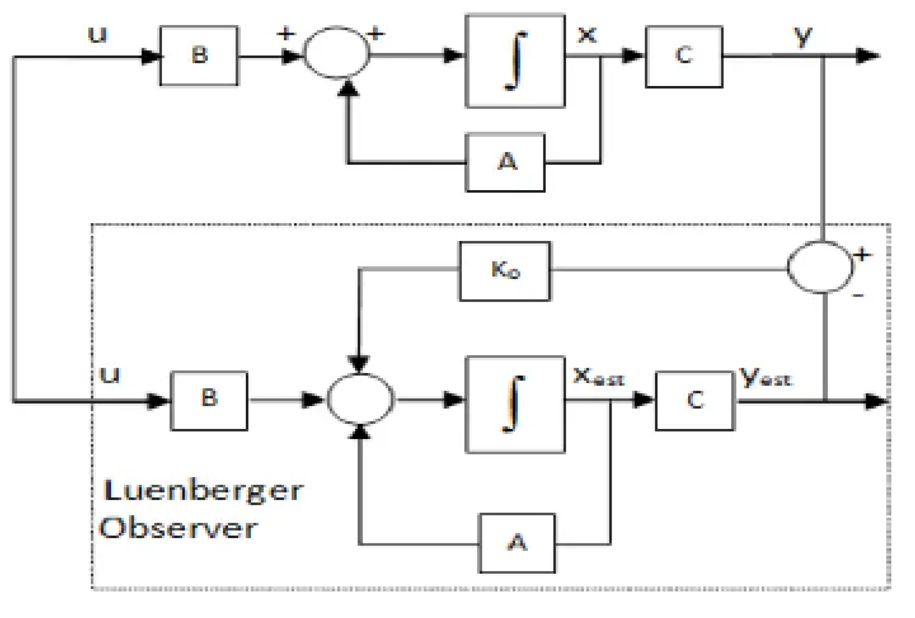
The basic idea of designing a Luenberger observer is to artificially build a system with the same parameters and inputs as the original system.

$$\{\begin{array}{l}\stackrel{·}{\widehat{x}}(t)=\mathrm{A}\widehat{x}(t)+\mathrm{B}u(t)+d(t)\\ \widehat{s}(t)=C\widehat{x}(t)\end{array}$$

(30)

The observation error at this time can be defined as

$$\tilde{x}=x-\widehat{x}$$

(31)

The error differential is

$$\stackrel{·}{\tilde{x}}=A(x-\widehat{x})$$

(32)

As can be seen from the above equation, without introducing feedback, the dynamics of the observed error are completely determined by system matrix A. If the characteristic roots of A are all on the left side of the complex plane, the observed error will approach zero with the passage of time. However, when the system itself is unstable, its zero pole needs to be configured by introducing feedback, and so the design of the Luenberger observer can be expressed as

$$\{\begin{array}{l}\stackrel{·}{\widehat{x}}(t)=\mathrm{A}\widehat{x}(t)+\mathrm{B}u(t)+L[\mathrm{s}(t)-\widehat{s}(t)]+d(t)\\ \widehat{s}(t)=C\widehat{x}(t)\end{array}$$

(33)

At this time, the dynamics of the observer error can be expressed as

$$\stackrel{·}{\tilde{x}}=(A-LC)\widehat{x}$$

(34)

Then, by selecting L, the characteristic root of the above formula is a proper value, thus ensuring that the error can be attenuated to zero and kept, and it is independent of the control input u(t) and the initial state x(0) of the system. In order to understand the Luenberger observer more vividly, we give its system block diagram. As shown in the Figure 3.

The Luenberger observer controls the observed measurement $x(t)$ by introducing linear feedback. The essence of its control is to make it possible to track $x(t)$.

5. Numerical Studies

REMUS AUVs are used as models for simulation tests. The parameters of the dive plane model of a REMUS are shown in the Appendix A. Choose the expected heave speed $w_d=0$, expected pitch speed $q_d=0$, expected pitch angle ${\theta }_d=0$, and expected depth $z_d=0\mathrm{m}$. Suppose the surge velocity $u=2\mathrm{m}/\mathrm{s}$, the initial state $w_0=0.02\mathrm{m}/\mathrm{s}$, $q_0=0.04\mathrm{r}\mathrm{a}\mathrm{d}/\mathrm{s}$, ${\theta }_0=0.1\mathrm{r}\mathrm{a}\mathrm{d}$, $z_0=10\mathrm{m}$.

Select switch function $C=diag[0.51-0.50-0.730.50]$, $K=0.65$, $\alpha =0.5$, $\sigma =0.85$, $d=[0.5 \sin (10t)0.5 \sin (10t{\left)00\right]}^T$. The following simulation results are obtained (Figure 4, Figure 5, Figure 6, Figure 7 and Figure 8):

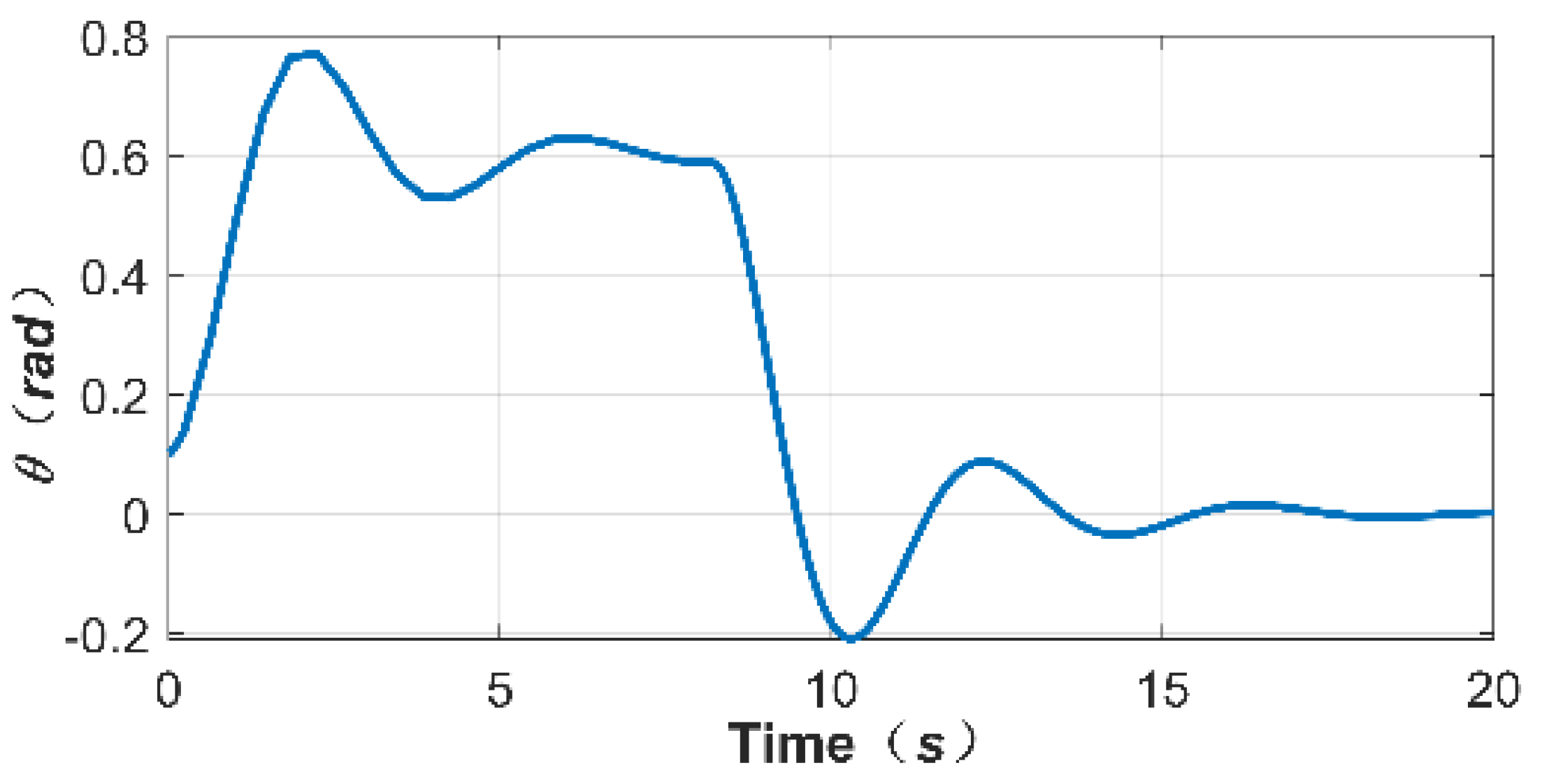
According to the tracking curve in Figure 4, Figure 5 and Figure 6 during the simulation process, it can be seen that the event-triggered sliding mode controller in the case of interference works stably and has good robustness. These characteristics mean the control task of AUV sailing depth can be completed. The observer coincides with the actual speed in a short time (within 5 s), which can feed the data back to the controller in time. 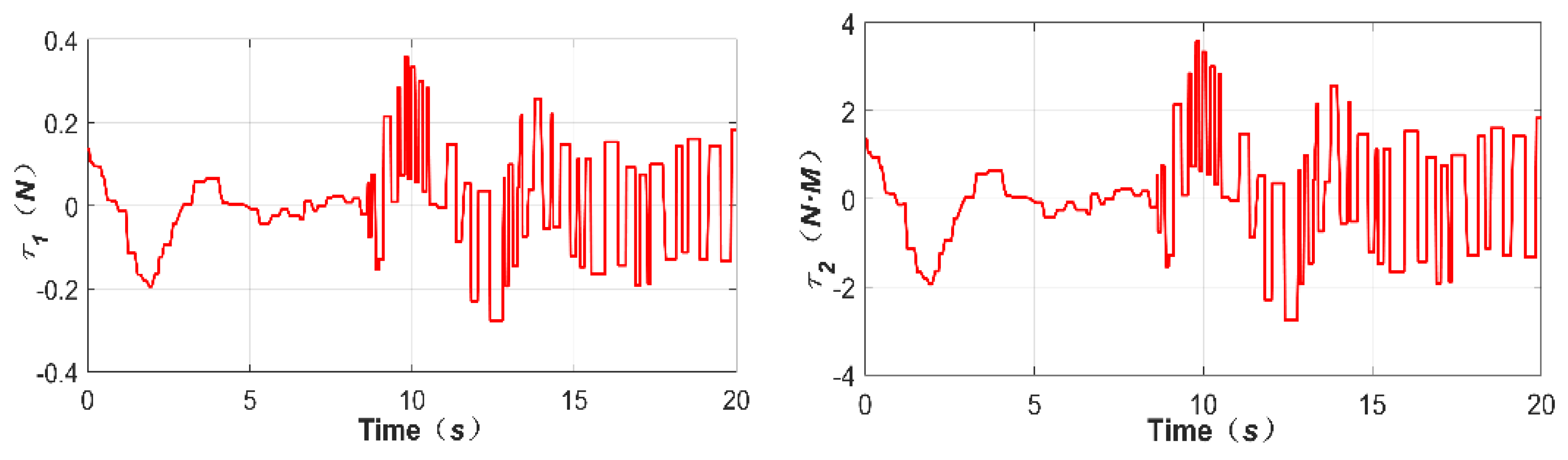Figure 8 shows the control input curve of the AUV system. It shown that the frequency of the change in control rate can be effectively reduced based on the action of event triggering. The event-triggered interval is shown in Figure 7. In the adjustment stage (0–10 s), due to a large system error, the event-triggered interval is short, while in the stability stage (10–20 s), the event-triggered interval is long, which can effectively reduce the energy loss caused by the change in control law.

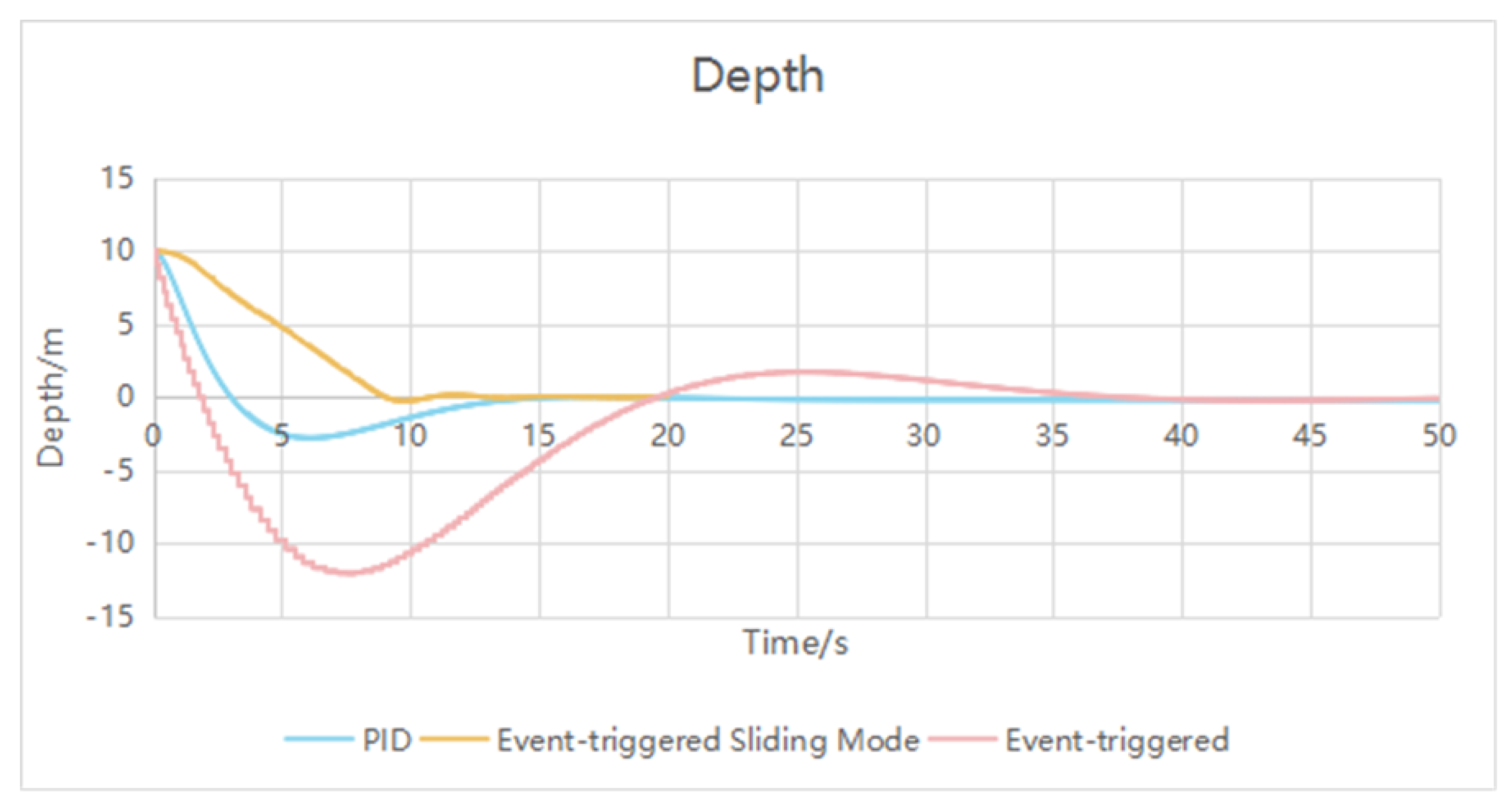
Taking a REMUS AUV as the research object, depth simulation experiments of various control methods are carried out, and the depth control effect of the sliding mode controller, based on event triggering, is compared and verified. As shown in the Figure 9.

In the 20 s simulation, there are 513 controls, of which 26 are triggered by events, accounting for about 5% of the total, which can achieve 5.07% energy saving. It can save 5.07% of computing resources. This is shown in the

Table 2. Event trigger times in simulation.

	Step Number	Percentage
Basic control step number	487	94.93%
Event step number	26	5.07%
Total number of steps	513	100%

below.

In the process of simulation, it can be seen that the PID controller can realize AUV depth control, but there is overshoot. It is stable for about 20 s, but it has a steady-state error of about −0.2 m.

In the simulation process, it can be seen that the event trigger controller can realize AUV depth control, and that it is stable for about 41 s. Although it can reduce the amount of calculation, it takes a long time to stabilize.

It can be seen from the comparison diagram that the sliding mode control based on event trigger can reach the desired depth faster, more accurately and more stably, and can achieve a 5% energy saving in calculation steps.

6. Outfield Experiment

In order to test the feasibility of the control law and ensure the safety of AUVs, the test site was selected in a water area of Shanghai. As shown in the Figure 10.

The expected depth is set at 0.8 m and 1 m, and the depth variation curve is shown in the following figure. As shown in the Figure 11 and Figure 12 and

Table 3. Event trigger times in outfield experiment.

	Step Number	Percentage
Basic control step number	9352	97.28%
Event step number	261	2.72%
Total number of steps	9613	100%

.

The outfield experiment proves that the controller can realize the expected depth control of AUV. It can save 2.72% of computing resources.

7. Conclusions

Aiming at the problem of improving the endurance of AUV in the inspection of long water conveyance tunnels, an energy-saving control method is proposed to realize the depth control of AUV, and an event-triggered sliding mode controller is designed. The controller only needs to send instructions to the next module (thrust distribution module) when some discrete events trigger, which can effectively reduce the energy consumption of the controller and achieve the purpose of AUV energy saving. The controller can effectively suppress the interference, realize the convergence of the state control error to a small invariant set containing the origin, and ensure that the whole system will not have Zeno phenomena. Compared with numerical simulation of PID and event-triggered control, this controller has the following advantages:

• Faster. It can reach the desired depth in a short time (10 s), while other methods can reach a better level in 15–35 s.
• More accurate. Too much or too little steady-state error will not occur when the desired depth is reached.
• More stable. There will be no overshoot when the desired depth is reached.
• Save computing resources. By transmitting only when some discrete events are triggered, the computing resources are saved. The simulation shows that the energy saving effect is 5.07%, and the field experiment shows that the energy saving effect is 2.72%.

The simulation results show that the sliding film controller based on event triggering is faster, more accurate, more stable and energy saving, and the field test proves the feasibility of the controller.

The development of a suitable experimental prototype can directly participate in the inspection of long water conveyance tunnels, save manpower, material resources and energy, and create direct economic value. It can also be used for other tasks, such as underwater terrain scanning and detection, water quality and environmental monitoring, etc. It can bring all kinds of direct or indirect economic benefits. In the research process, the combination of industry–university–research is expected to bring various economic benefits, and especially to bring various benefits to enterprises and scientific research projects. After the technology is patented, it can also be used in the design of other robots such as surface robots and land robots. It can also be used in industrial robots, aviation and other fields.