
Magnetic Plug Sensor with Bridge Nonlinear Correction Circuit for Oil Condition Monitoring of Marine Machinery

 , , , ,
Abstract
:1. Introduction
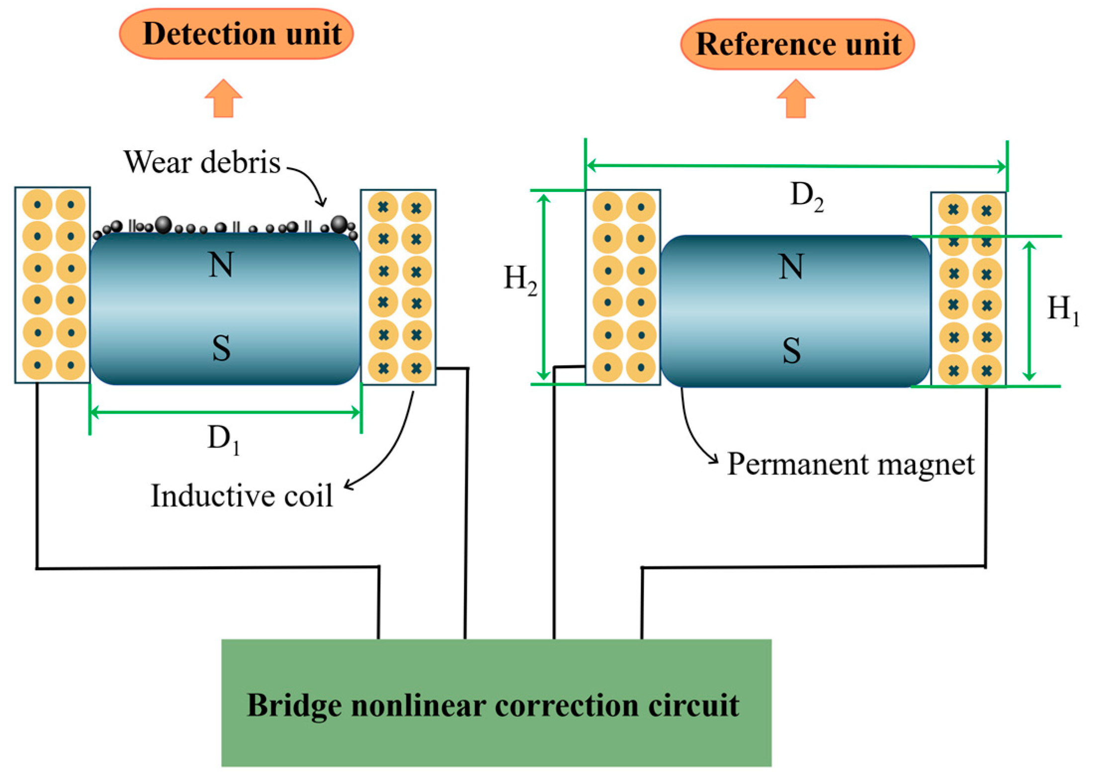
2. Magnetic Plug Sensor Design
2.1. Strutural Optimization
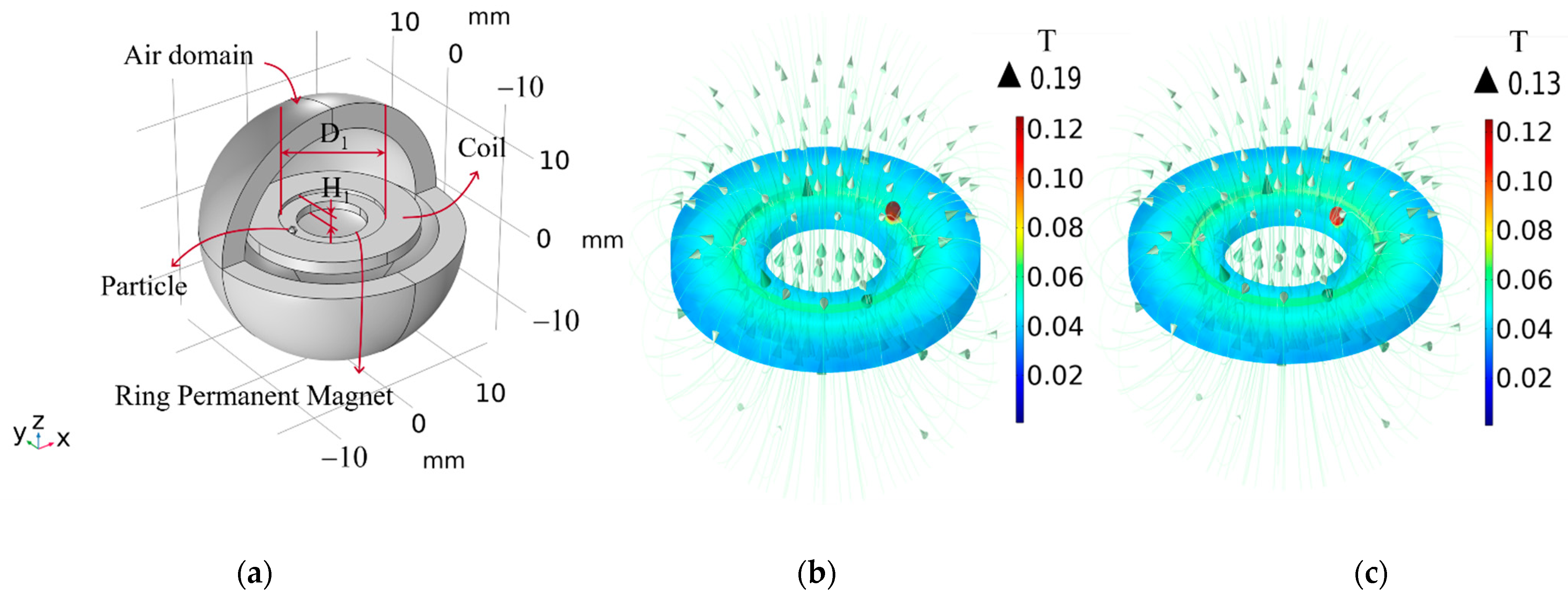
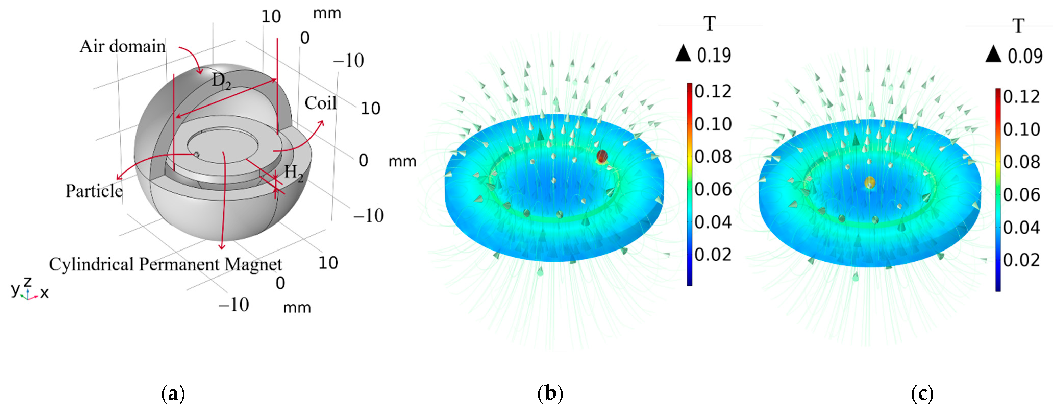
2.1.1. Details of Finite Element Analysis
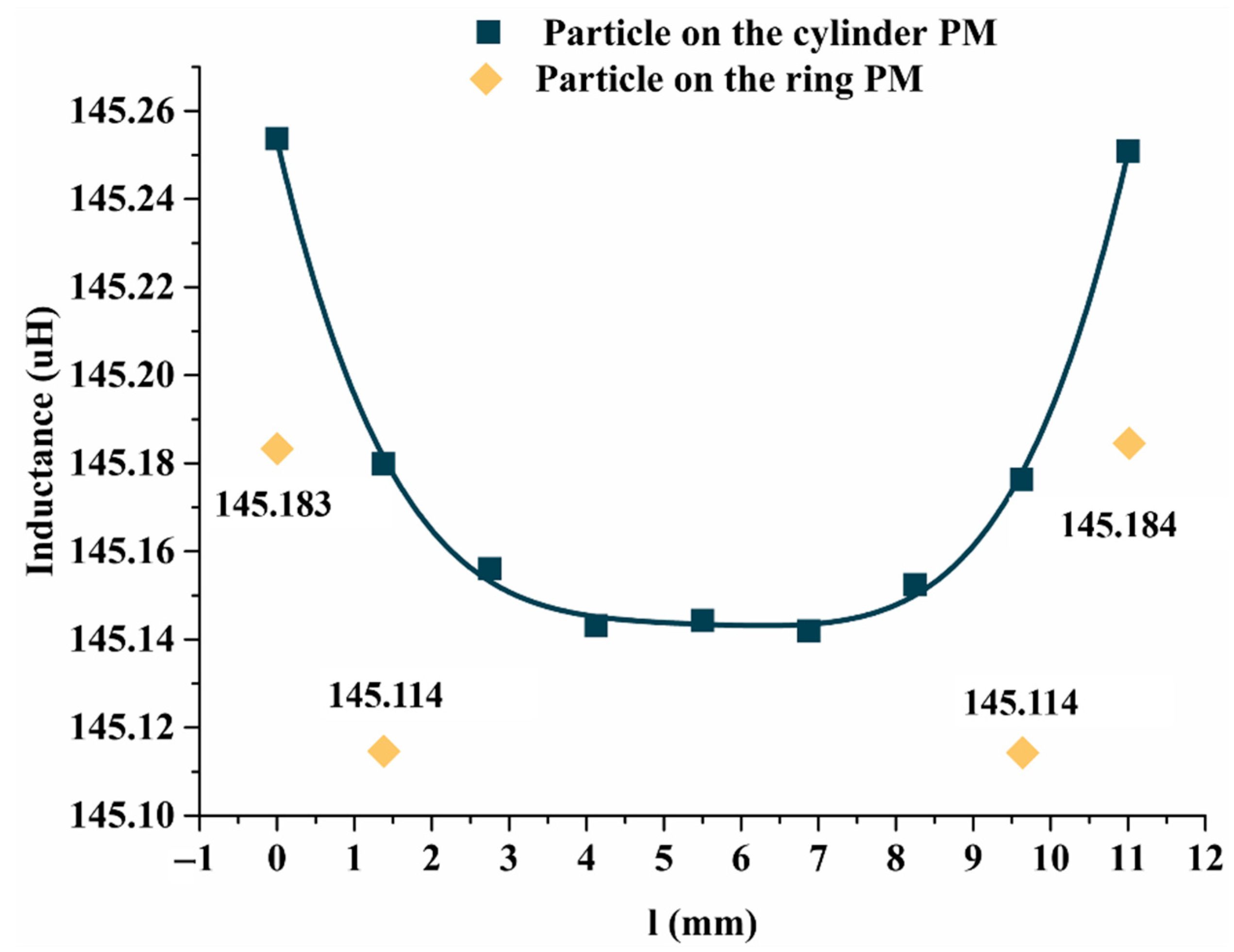
2.1.2. Results of Finite Element Analysis
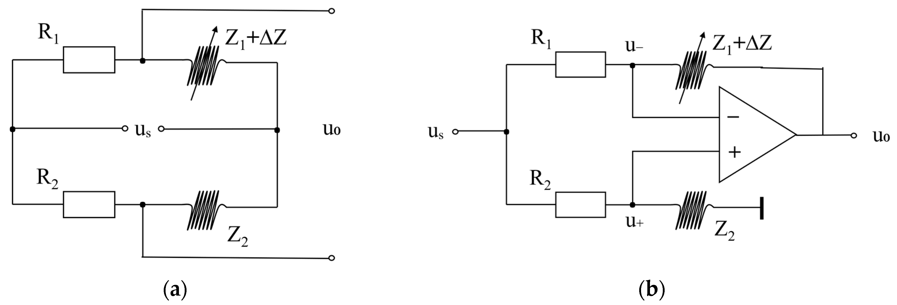
2.2. Bridge Nonlinear Correction Circuit
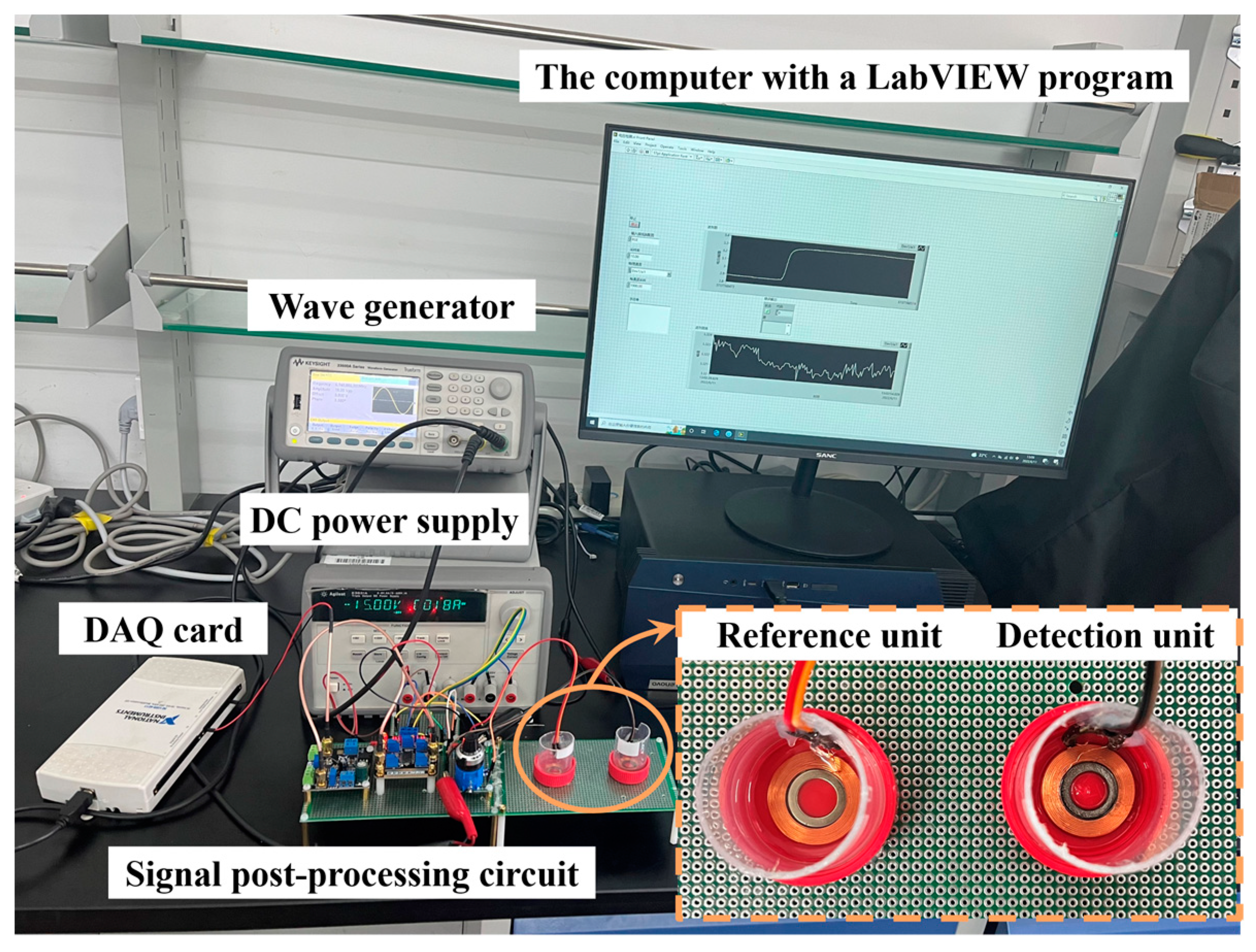
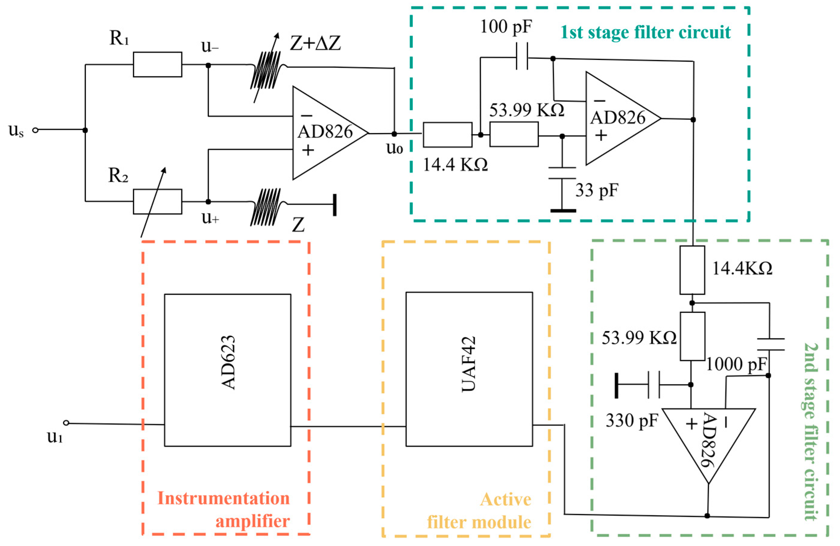
3. Detection System and Circuit
4. Experiment and Discussion
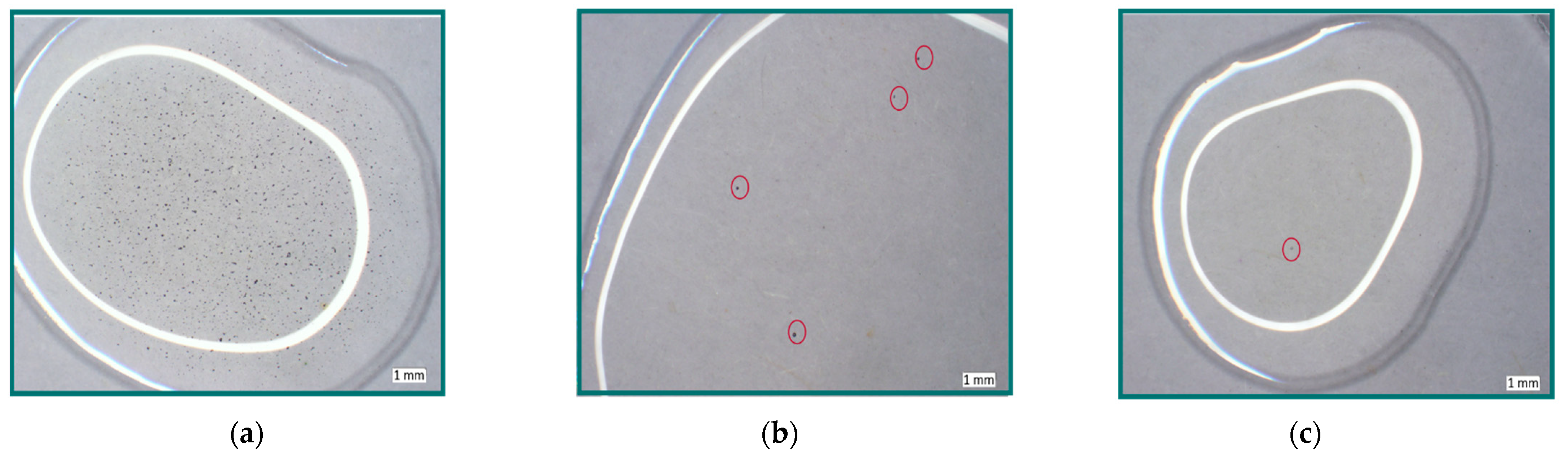
4.1. Void Test
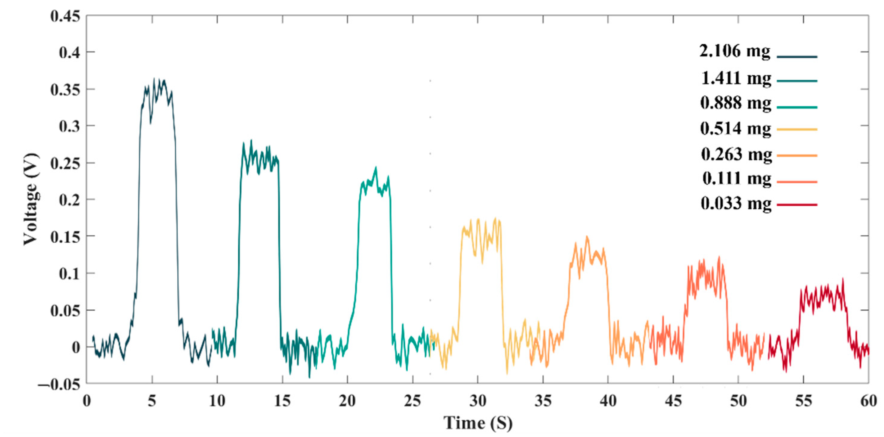
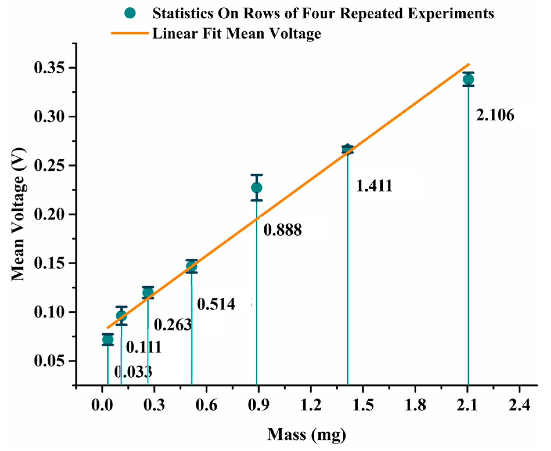
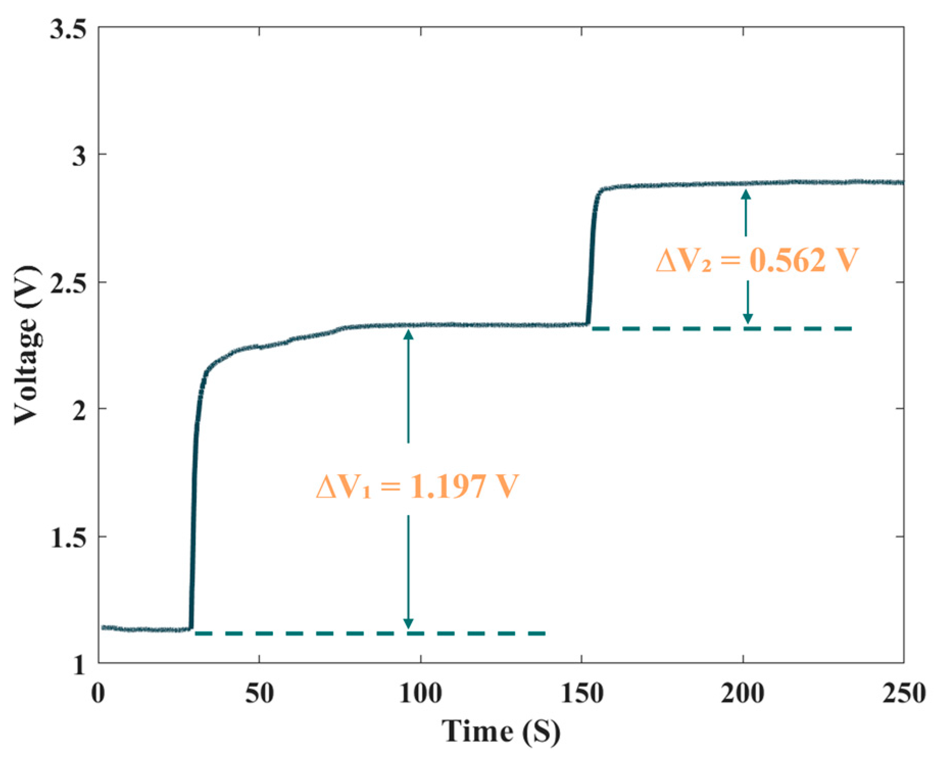
4.2. Dynamic Test
4.3. Discussion
5. Conclusions
Author Contributions
Funding
Institutional Review Board Statement
Informed Consent Statement
Data Availability Statement
Conflicts of Interest
References
- Liang, X.H.; Zou, M.J.; Feng, Z.P. Dynamic modeling of gearbox faults: A review. MSSP 2018, 98, 852–876. [Google Scholar] [CrossRef]
- Fan, B.; Li, B.; Feng, S.; Mao, J.; Xie, Y.B. Modeling and experimental investigations on the relationship between wear debris concentration and wear rate in lubrication systems. Tribol. Int. 2017, 109, 114–123. [Google Scholar] [CrossRef] [Green Version]
- Sun, J.; Wang, L.; Li, J.; Li, F.; Li, J.; Lu, H. Online oil debris monitoring of rotating machinery: A detailed review of more than three decades. MSSP 2021, 149, 107341. [Google Scholar] [CrossRef]
- Zhu, X.L.; Zhong, C.; Zhe, J. Lubricating oil conditioning sensors for online machine health monitoring—A review. Tribol. Int. 2017, 109, 473–484. [Google Scholar] [CrossRef] [Green Version]
- Xi, W.; Wu, T.; Yan, K.; Yang, X.; Jiang, X.; Kwok, N. Restoration of online video ferrography images for out-of-focus degradations. J. Image Video Process. 2018, 2018, 31. [Google Scholar] [CrossRef]
- Mehri, T.; Kemppinen, O.; David, G.; Lindqvist, H.; Tyynelä, J.; Nousiainen, T.; Rairoux, P.; Miffre, A. Investigating the size, shape and surface roughness dependence of polarization lidars with light-scattering computations on real mineral dust particles: Application to dust particles’ external mixtures and dust mass concentration retrievals. Atmos. Res. 2018, 203, 44–61. [Google Scholar] [CrossRef]
- Amann, S.; Witzleben, M.V.; Breuer, S. 3D-printable portable open-source platform for low-cost lens-less holographic cellular imaging. Sci. Rep. 2019, 9, 11260. [Google Scholar] [CrossRef] [PubMed] [Green Version]
- Schoell, R.; Xi, L.; Zhao, Y.; Wu, X.; Yu, Z.; Kenesei, P.; Almer, J.; Shayer, Z.; Kaoumi, D. In situ synchrotron X-ray tomography of 304 stainless steels undergoing chlorine-induced stress corrosion cracking. Corros. Sci. 2020, 170, 108687. [Google Scholar] [CrossRef]
- Jin, Z.; Zhang, F.Q. Analysis of spatial sensitivity based on electrostatic monitoring technique in oil-lubricated system. Open Access Libr. J. 2018, 5, 1–13. [Google Scholar] [CrossRef]
- Qian, M.; Ren, Y.J.; Zhao, G.F.; Feng, Z. Ultrasensitive inductive debris sensor with a two-stage auto asymmetry compensation circuit. IEEE TIE 2021, 68, 8885–8893. [Google Scholar]
- Muthuvel, P.; George, B.; Ramadass, G.A. A Highly Sensitive In-Line Oil Wear Debris Sensor Based on Passive Wireless LC Sensing. IEEE Sens. J. 2021, 21, 6888–6896. [Google Scholar] [CrossRef]
- Harkemance, E.; Berten, O.; Hendrick, P. Analysis and Testing of Debris Monitoring Sensors for Aircraft Lubrication Systems. Proceedings 2018, 2, 416. [Google Scholar]
- Itomi, S. Oil Condition Sensor. U.S. Patent US7151383 [P], 26 September 2006. [Google Scholar]
- Muthuvel, P.; George, B.; Ramadass, G.A. Magnetic-Capacitive Wear Debris Sensor Plug for Condition Monitoring of Hydraulic Systems. IEEE Sens. J. 2018, 18, 9120–9127. [Google Scholar] [CrossRef]
- Cao, Y.; Liu, R.; Du, J.; Yu, F.; Yang, Q.; He, Y.; Li, S. Gas Turbine Bearing Wear Monitoring Method Based on Magnetic Plug Inductance Sensor. In Proceedings of the 2018 13th ICST, Oslo, Norway, 11–15 June 2018. [Google Scholar]
- Muthuvel, P.; George, B.; Ramadass, G.A. A planar inductive based oil debris sensor plug. In Proceedings of the 2019 13th ICST, NSW, Australia, 2–4 December 2019. [Google Scholar]
- Shi, H.T.; Bai, C.Z.; Xie, Y.C.; Li, W.; Zhang, H.; Liu, Y.; Zheng, Y.; Zhang, S.; Zhang, Y.; Lu, H.; et al. Capacitive–Inductive Magnetic Plug Sensor with High Adaptability for Online Debris Monitoring. IEEE TIM 2022, 71, 1–8. [Google Scholar] [CrossRef]


| Cylindrical Type | Ring Type | |
|---|---|---|
| value 1 (μH) | 0.232 | 0.098 |
| absolute deviation (μH) | 0.073 | 0.035 |
| Oil Sample | Diameter (μm) | Mass (mg) |
|---|---|---|
| S1 | 200 | 0.033 |
| S2 | 300 | 0.111 |
| S3 | 400 | 0.263 |
| S4 | 500 | 0.514 |
| S5 | 600 | 0.888 |
| S6 | 700 | 1.411 |
| S7 | 800 | 2.106 |
| Author | Dynamic Test | Void Test | Linearity | Particle Location Impact | Ref. |
|---|---|---|---|---|---|
| Harkemance, E. | 10 mg | - | - | - | [12] |
| Itomi, S. | 20 mg | - | - | - | [13] |
| Muthuvel, P. | 10 mg | - | - | - | [14] |
| Cao, Y.P | 100 mg | - | - | - | [15] |
| Muthuvel, P. | 10 mg | - | - | - | [16] |
| Shi, H.T. | - | 200 um | N | Big | [17] |
| Our work | 2.5 mg | 200 um | Y | A little |
Publisher’s Note: MDPI stays neutral with regard to jurisdictional claims in published maps and institutional affiliations. |
© 2022 by the authors. Licensee MDPI, Basel, Switzerland. This article is an open access article distributed under the terms and conditions of the Creative Commons Attribution (CC BY) license (https://creativecommons.org/licenses/by/4.0/).
Share and Cite
Zhang, Y.; Hong, J.; Shi, H.; Xie, Y.; Zhang, H.; Zhang, S.; Li, W.; Chen, H. Magnetic Plug Sensor with Bridge Nonlinear Correction Circuit for Oil Condition Monitoring of Marine Machinery. J. Mar. Sci. Eng. 2022, 10, 1883. https://doi.org/10.3390/jmse10121883
Zhang Y, Hong J, Shi H, Xie Y, Zhang H, Zhang S, Li W, Chen H. Magnetic Plug Sensor with Bridge Nonlinear Correction Circuit for Oil Condition Monitoring of Marine Machinery. Journal of Marine Science and Engineering. 2022; 10(12):1883. https://doi.org/10.3390/jmse10121883
Chicago/Turabian StyleZhang, Yuwei, Jiaju Hong, Haotian Shi, Yucai Xie, Hongpeng Zhang, Shuyao Zhang, Wei Li, and Haiquan Chen. 2022. "Magnetic Plug Sensor with Bridge Nonlinear Correction Circuit for Oil Condition Monitoring of Marine Machinery" Journal of Marine Science and Engineering 10, no. 12: 1883. https://doi.org/10.3390/jmse10121883