Hydrology and Dynamics in the Gulf of Naples during Spring of 2016: In Situ and Model Data

Abstract

The hydrology and circulation in the northwestern part of the Gulf of Naples are analyzed during the transition period from spring to summer (April–June) 2016 through numerical simulations and in situ observations. The simulations were performed with the high-resolution sigma-coordinate Campania Regional Ocean Model (CROM) encompassing the wider Campania coastal system. Temperature, salinity and density were measured at the Long Term Ecological Research Program Mare-Chiara sampling site located two miles from the coast, while current intensity and direction were measured in situ by an acoustic Doppler current profiler connected to an elastic beacon anchored at a short distance from the city of Naples. The modeled circulation scenarios and the marine hydrology provided by the model on a regular grid allow interpreting the observational data during the selected period. In turn, the model-data comparison clarifies the model performance in reproducing the nearshore marine dynamics, which goes beyond the actual model resolution.

1. Introduction

The Gulf of Naples (GN hereafter) is a semi-enclosed bay (Figure 1) located on the western coasts of southern Italy along the Tyrrhenian Sea (TS) and is characterized by a complex orography and the presence of islands and straits (e.g., [1,2,3,4,5]). Regarding the TS circulation, see the recent review of Iacono et al. [6]; for specific features, see the work Falco et al. and Krauzig et al. [7,8].

Many anthropic activities take place along the GN coasts, potentially determining a strong impact on the marine ecosystem [9]. These activities range from intense maritime traffic (the harbor of Naples is one of the most important harbors in the Mediterranean both in width and maritime traffic [10]) to urban settlements, tourism and industrial areas located on the coast, resulting in the potential discharge of sewage, industrial pollutants and hydrocarbons [11]. In addition, the eastern part of the GN receives the land runoff of the Sarno, a very polluted river carrying a heavy load of sediment and suspended matter that can influence the physical, chemical and biological quality of the coastal waters [4]. Moreover, the presence of several archaeological sites [12] also calls for studies on the dynamics and on hydrological characteristics of this area in order to preserve their features and beauty.

Several modeling studies have been carried out so far [13,14,15,16,17,18,19,20], emphasizing the spatiotemporal complexity of the water dynamics in this area. In the work of de Ruggiero et al. [17], the authors have implemented the high-resolution Campania Regional Ocean Model (CROM) and have focused on the important interaction between the Tyrrhenian-scale circulation and the dynamics along the Campania coastal system (CCS), through the analysis of the winter and summer 2009 scenarios. In addition, the importance of local wind-induced flow, which can generate inertial currents offshore, as well as breeze-induced currents within the gulfs of the CCS was also analyzed. In the work of de Ruggiero et al. [18], the first comprehensive assessment of the marine circulation variability in the CCS through the analysis of twelve-monthly hindcasts carried out with CROM for 2016 was also carried out.

The oceanographic observations provide high accuracy, but the resulting information is limited since they involve fixed point measurements [21]. At the same time, sensor malfunctioning (even over long periods of time) can lead to discontinuity in the dataset and thus loss of information. In addition, the large efforts spent on in situ point measurements are often of limited use for ocean model validation [21]. One reason for this is that such observations often lack information on short-term variability in either time or space, or both (e.g., while an observational buoy may provide almost continuous observations in time, there is no information on how representative these observations are in space).

In this context, remote sensing data can complement traditional field measurements, providing near-continuous synoptic coverage with a good trade-off between spatial and temporal resolution, thus enabling timely characterization of physical and biological dynamics within the upper layer of the ocean [22]. An illustration of the application of this methodology in the area is provided in [2,7,23,24] in which an investigation was performed on the surface dynamics using data provided by a land-based remote sensing system (HF coastal radar). Moreover, HF radar data assimilation into coastal circulation models can greatly improve the model performance in an operational context [25,26].

The ocean model simulations are continuous in time and space and allow both understanding larger-scale marine dynamics and identifying basin-scale features that are difficult to derive from point measurements. High-resolution ocean models may connect sparse observations, synthesize them and assist the design of observational networks [27]; in turn, observations can guide coastal model development and calibration [27] and may highlight the limits of the model simulations. Thus, integration and synergy between observations and models can add value to coastal monitoring and enable a variety of applications [28], including search and rescue, pollutant transport processes, sustainability of coastal ecosystems, safety of coastal populations and sea level rise monitoring.

However, as pointed out in [29], modeling coastal dynamics is perhaps the most complex challenge from a modeling point of view since several processes (tidal forcing, irregular shoreline and bathymetry, wind forcing, freshwater discharges and fluvial inputs) play an important role and influence the current dynamics and hydrology. In addition, the limitation in available forcings (atmospheric, freshwater, tidal as well as bathymetric resolution) generates discrepancies between the modeled results and observations. Moreover, the model performance could also decrease due to topographic smoothing that results from the filtering of some relevant local bottom features near the coast [21].

In this context, the present work is aimed to study the marine dynamics within the GN by combining an observational dataset with a simulated one. We focus on the analysis of the dynamics of the GN during spring 2016, particularly in its northern sector commonly referred to as the Bay of Naples (BN), using an integrated approach that requires the use of both numerical simulations (the hindcasts provided in [18] are used) and meteo-oceanographic time series data collected at two fixed observation points in the BN (the Long Term Ecological Research Program Mare-Chiara (LTER-MC) and an acoustic Doppler current profiler connected to an elastic beacon (MEDA B)).

The choice of the spring season is due to the interesting variability of water masses, which show the transition from winter to summer conditions. During spring, the strong northwestward Tyrrhenian current, which is the prevailing driving force of the circulation patterns within the GN during the winter period, becomes unstable due to the weakening of the cyclonic wind-stress curl; the local forcing becomes, therefore, the main driver of the water masses within the basin, and the formation of an anticyclonic circulation within the GN is found (see [18,30]). From a biological perspective, with maximum daylength and thermal stratification of the water column in late spring–early summer, the phytoplankton population attains its maximum concentrations in this period of the year [31].

The circulation scenarios and the hydrology produced by the model allow interpreting the observational data during the selected period. Monthly mean circulation scenarios detect northeastward surface current patterns in agreement with observations, despite the reduced intensity of the simulated surface current field due to the weaker wind stress used to force the model. The rotary spectral and harmonic analysis show that the tidal contribution is negligible within the GN [2,4] and that the breeze regime drives the dynamics over the study period. In addition, the empirical orthogonal function (EOF) analysis of the basin-scale simulated current field highlights the occurrence of the inertial component in the rotational spectrum for the expansion coefficients, which, however, is not so prominent from the analysis of the observed dataset.

The hydrological data analyses confirm that the study area is affected by lateral advection of freshwater that leads to a decrease in surface salinity, thus enhancing the water column stability, as reported in previous studies (e.g., [32]). The causes that produce departures of the model simulations from the observed data and potential improvements of model setting are also discussed.

The present study is organized as follows: In Section 2, descriptions of the in situ data, the model implementation and the analyses carried out are provided. In Section 3, we focus on the obtained results: marine hydrology, meteorology and sea current dynamics for April, May and June 2016 are described in detail. Section 4 presents the analysis of the modeling data and their comparison with the observed data. Finally, conclusions are outlined in Section 5.

2. Materials and Methods

2.1. In Situ Data

In this section, we describe the in situ hydrological, meteorological and current meter data used to analyze the selected period of April to June 2016 (5 April 2016–30 June 2016).

To avoid any ambiguity, we would like to clarify that under the term hydrology we mean the main physical parameters of the water column, namely the temperature, salinity and density.

Time series of temperature (T), salinity (S) and density ($\mathsf{\rho })$ were recorded at the LTER-MC (40.81° N–14.25° E) fixed sampling site, located two miles off the coast of Naples at a depth of 75 m (blue star in Figure 1b). Since January 1984, marine plankton samples and hydrological data have been collected and studied by the Stazione Zoologica A. Dohrn [32,33,34]. From 1984 to 1991, the sampling rate was biweekly, becoming weekly starting from February 195. This large dataset allowed us to analyze the seasonal evolution and the typical trends of the marine area of the BN. The hydrological parameters were acquired with a conductivity–temperature–depth (CTD) recording instrument (see

Table 1. CTD unit technical parameters.

Site	LTER-MC
CTD	SBE 9 plus V2
Deck Unit	SBE 11 plus V2
(2X) Temperature	SBE 3 plus
(2X) Conductivity	SBE 4
PAR	Biospherical QSP
Dissolved Oxygen	SBE 43
pH-ORP	SBE 27
Fluorometer	Chelsea Aqua mk3
Transmissometer	Wet Labs C-Star (20 cm)

for the technical parameters; for further details, see Profiling | Sea-Bird Scientific-Overview | Sea-Bird (seabird.com, accessed on 13 July 2020)).

The MEDA B elastic beacon (red star in Figure 1b) of the BN (40.82° N–14.23° E) is equipped with automatic instruments for the continuous acquisition of the meteorological and marine parameters, which allowed us to carry out high-frequency and long-term measurements. The following meteorological parameters were analyzed: air temperature, atmospheric pressure, relative humidity and wind direction and speed.

The current meter data were acquired by an acoustic Doppler current profiler (ADCP) (see

Table 2. ADCP configuration parameters.

Site	Meda B Napoli
Model	ADCP-600 khz
Water depth	18 m
Top bin depth	1.40 m
Bin size	50 cm
Mooring type	Bottom-mounted
Orientation	Upward looking
Latitude	40.8278° N
Longitude	14.2330° E

for configuration parameters) probe located on the seabed (about 17 m) and connected to the MEDA B buoy. The ADCP probe acquires the following parameters: direction and intensity of the current, direction of the wave motion and sea surface elevation. Speed profiles are divided by the ADCP into layers of uniform thickness called bins, and each bin corresponds to a specific depth cell. In this case, the 600 khz ADCP probe acquires 49 bins of 50 cm thickness (vertical resolution). The center of the first bin is 1.6 m from the transducer, which in turn is about 50 cm from the seabed, so the center of the first bin is 2.10 m from the sea bottom. The 30th bin is chosen as a reference for the surface values of direction and intensity of the sea current (1.40 m from the sea surface).

2.2. The Model

The CROM (for details, see [17]) is based on the Princeton Ocean Model (POM [35]). The model is implemented on a coastal zone of the southern TS defined as the CCS [15] that includes the GN, as well as the gulfs of Gaeta and Salerno, with a horizontal spatial resolution of 1/144° (Δy ≈ 772 m, Δx ≈ 579–591 m) on 40 sigma vertical levels. The CROM domain with bathymetry is shown in Figure 1a.

CROM is one-way nested with the NEMO-OPA (Nucleus for European Modeling of the Ocean-Ocean Parallelise [36]) model, implemented over the whole Mediterranean Sea with a 1/16° horizontal resolution and 71 unevenly spaced vertical levels [37]. The nesting technique used is described in detail in [17]. CROM is forced by momentum, heat, freshwater and radiative fluxes (with 5 km horizontal resolution) computed from the outputs of the non-hydrostatic SKIRON/Eta atmospheric modeling system (http://forecast.uoa.gr/forecastnewinfo.php, accessed on 27 April 2017) of the National and Kapodistrian University of Athens, using classical bulk formulae (see [38]). The hindcast outputs from April to June 2016, produced as described in [18], are here analyzed in combination with in situ data to study the marine dynamics during the transition from spring to summer period.

2.3. Analysis Methods

A preliminary validation of the dataset was first carried out to identify data values without significance both from a statistical and a physical point of view.

A basic qualitative and statistical analysis carried out on the observed dataset allows us to draw a general picture that enables us to characterize the spring dynamics affecting the BN from the meteorological, physical and dynamical points of view. In order to identify the time scales and the modes of variability of the flow in the water column investigated by the ADCP probe, a rotary spectral analysis [39] technique was applied both to the hourly near-surface current and to the wind stress time series (regarding the wind stress, due to lack of data we excluded June from our analysis). To ensure the continuity of the dataset and thus to satisfy the fast Fourier transform (FFT) requirement, a linear interpolation was previously applied to fill the gaps within the data records. Thus, the current and wind stress complex velocity records were Fourier transformed to clockwise (negative frequency) and counterclockwise (positive frequency) rotary components [39,40].

The wind stress components were obtained following [41] by using the following relations:

$$u_w={\rho }_a{c}_d\left|U\right|u$$

(1)

$$v_w={\rho }_a{c}_d\left|U\right|v$$

(2)

where U is the wind velocity, ${\rho }_a$ is a reference air density (1.3 kg/m³) and c_d is the drag coefficient calculated as in [41]:

$${\{\begin{array}{c}{c}_d={10}^{-3}, \left|U\right|\le 6 \mathrm{m}/\mathrm{s}\\ c_d=(0.61+0.063\ast \left|U\right|)/1000, 6 \mathrm{m}/\mathrm{s}<\left|U\right|\le 22 \mathrm{m}/\mathrm{s} \\ c_d=2\ast {10}^{-3} , 22 \mathrm{m}/\mathrm{s}<\left|U\right| \end{array}}_{ }$$

A least-squares tidal analysis (LSHA) technique was applied to both non-interpolated hourly surface ADCP data and wind stress time series in order to extract the astronomical contribution to the current variance and to detect periodicities in the local forcing. The harmonic analysis was performed by using the MATLAB t_tide code [42]. Tidal ellipse parameters (major and minor axes, inclination and phase angle), together with their uncertainties, were obtained for each tidal constituent. Only tidal constituents with a signal-to-noise ratio (SNR) greater than or equal to 2 were reported.

To identify the dominant vertical modes of variability of sub-surface currents, empirical orthogonal function (EOF) analysis was performed on the hourly time series of ADCP current profiles. The EOF was used to explore the driving forces and spatiotemporal scales behind the variability of sea currents [43]. The representative spatial patterns (or EOF modes) and their corresponding temporal coefficients or principal components (PCs, which describe the evolution of the modes) were determined by solving the eigenvalue problem for the spatial covariance matrix. In detail, these simple steps were followed:

• Form the matrix from the observations, and remove the time mean of each time series;
• Find the covariance matrix;
• Find the eigenvalue and eigenvector of the covariance matrix;
• Find the largest eigenvalues and their corresponding eigenvectors, the EOFs;
• Find the expansion coefficient.

Moreover, a spectral analysis was performed on the obtained principal component time series.

To relate the current to some particular wind conditions, the high-frequency current motions were eliminated by low-pass filtering. A digital symmetric low-pass filter (PL33), was applied to the wind stress and current time series [44]. Then the complex cross-correlation function [43] was used to evaluate how the surface current at a generic time depended on the wind stress acting at the same and at previous times.

The modeling results were used to investigate the spring dynamics, using the same approach adopted for the observed dataset, but with an emphasis on basin-wide dynamics. Again, the tidal and frequency analysis was applied both to spatially hourly averaged surface current and to wind stress modeling data in the BN area to highlight similarities and differences from the observed spectra. Moreover, the EOF analysis was applied both to the vertical simulated current profile in the BN and to the surface current field at the basin scale to identify its spatiotemporal variability and its wind response. In addition, the hindcast results were statistically compared with the observed dataset to verify how closely the modeled results matched the physical and dynamical features of the area. For this purpose, the vertical profiles (T, S and $\mathsf{\rho }$ in a 70 m water column) observed at the LTER-MC sampling site and the current field measured by the ADCP probe were compared with those simulated by CROM. The simulated vertical profiles were spatially averaged over 37 grid points. Simulation data are provided on 40 sigma levels; thus, to make the measurements comparable, linear interpolation on equidistant zeta levels (vertical resolution of 1 m) was performed.

It is worth stressing that here we do not aim to validate the employed oceanic model, since the obtained comparison results may be altered by both the lack of a continuously observed dataset and the extremely close distance to the coast of the sensors and measurements. Instead, the comparison suggests improvements in the model implementation in such a small and peculiar area.

3. In Situ Data Results

3.1. Hydrological and Meteorological Conditions

The hydrological data have been collected weekly at the LTER-MC sampling site; the Hovmöller diagrams of Figure 2 allow us to describe the vertical and temporal variability of S, T and $\mathsf{\rho }$ acquired by the CTD probe at the LTER-MC sampling point from April to June 2016. Salinity (Figure 2a) increases with depth, showing values in the range 36.99–38.18 PSU. Occasional surface nuclei of freshwater are observed on 12 April, 18 May and 21 June (perhaps due to some spillage phenomenon or freshwater input that reached the area). As assessed in [32], lateral advection of fresher water from the coast frequently determined a decrease in surface salinity, resulting in a sharp halocline. In stratified conditions, low-salinity waters floated at the surface, thereby enhancing the water column stability and reducing the mixed layer depth. Temperature (Figure 2b) decreases with the increase in water depth, reaching minimum values of 14–15 °C near 70 m. Surface temperature obviously increases with time, progressing towards the summer, and the Hovmöller diagram clearly shows a downward propagation of this signal. The maximum surface temperature is recorded in June with values of about 25 °C (8 °C more than the maximum surface temperatures measured in April). Similarly, the density (Figure 2c) increases proportionally to the depth, determining the stratification of the water column shown in June; the density behavior is primarily driven by temperature, apart from the above-mentioned occasional surface intrusions of fresher water which result in transient density reductions.

Table 3. Hydrological main statistical parameters.

	Max	Min	Std	Median
Temperature (°C)	24.9	14.8	2.1	15.6
Salinity (PSU)	38.1	36.9	0.1	37.9
Density (kg/m3)	1028.4	1025.2	0.6	1028.1

summarizes the main statistical parameters for the total study period, regarding the hydrological dataset described above.

The meteorological dataset measured at MEDA B Napoli buoy has a one-hour sampling rate. In Figure 3, we can see the time series evolution of air temperature (T_a), air pressure (P_a) and relative humidity (R_h) for the April–June quarter. Superimposed on the hourly time series, we report the daily (blue line in Figure 3) and weekly (red line in Figure 3) time series moving averages, which, in accordance with the Mann–Kendell test, are statistically significant. With reference to T_a (Figure 3a), the maximum value (30.3 °C) was recorded on 16 June 2016 at 08:00 AM while the minimum value (9.3 °C) was recorded on 25 April 2016 at 6:00 AM. On average, values of 17.06 °C were recorded. With reference to P_a (Figure 3b), the maximum value (1023.2 hpa) was recorded on 21 April 2016 at 11:00 AM. The minimum was recorded on 8 April 2016 at 4:00 AM, with a value of 996.8 hPa. Overall, there was an average of 1012.9 hPa. With reference to R_h (Figure 3c), the maximum value (88.6%) was recorded on 22 April 2016 at 6 PM while the minimum value (22.8%) was recorded on 20 April 2016 at 7:00 PM. In the entire survey period, there was an average of 64%.

Wind rose diagrams (Figure 4a,b) show the observed wind features. The maximum wind speed was recorded on 12 May 2016 with a value of 11.42 m/s (force 6, see

Table 4. Percentage of the wind speed range according to Beaufort scale.

Beaufort Scale (Force)	Descriptive Term	Wind Speed (m/s)	April (%)	May (%)
0	Calm	<0.3	2	1
1	Light breeze	0.3–1.5	23	21
2	Gentle breeze	1.6–3.3	26	23
3	Moderate breeze	3.4–5.5	24	29
4	Fresh breeze	5.6–7.9	22	18
5	Strong breeze	8–10.7	2	7
6	Near gale	10.8–13.8	1	1
7	High wind	>13.8	0	0

); the minimum was recorded around 06 April 2016 with a value of 0.12 m/s (force 0, see Table 4). There are no data for June. From the wind rose diagrams shown in Figure 4, it emerges that the prevailing wind direction for both April (Figure 4a) and May (Figure 4b) is from WSW. As assessed in different works [2,23] under this wind condition, surface waters were pushed towards the coast.

The wind conditions over the northern part of the GN were also determined using the Beaufort wind force scale. The results of this classification are presented in Table 4. As shown in Table 4, the highest frequency of wind speed belongs to the light breeze and fresh breeze scales (between force 1 and force 4), both for April and May wind datasets. Wind strength greater than 10.8 m/s (force 6) occurred about less than 1% both for April and May wind datasets and, generally, during the passage of significant low-pressure systems (minimum near 1000 hPa, see also Figure 3b). The maximum hourly mean value was recorded on the 24–25th of April 2016 (10.9 m/s) and on the 12th, 13th and 14th of May 2016 (wind speed about 11.4 m/s) when the pressure dropped to near 1000 hPa.

3.2. Sea Current Analysis

The analysis of the current intensity and direction acquired by the ADCP is shown in Figure 5. In this case, the current meter dataset has a 15 min sampling rate. To summarize the information recorded by the ADCP, we here used Hovmöller diagrams [45]. For the sake of clarity, data are reported with a 6 h sampling rate. Overall, the current intensity presents the highest values in the surface layers, while showing slightly lower values near the deep layers, where the frictional forces decrease the intensity of the flow. When the wind stress is greatest, we observe more intense currents even below the surface layer (see for example the high current speed value in the red box of Figure 5a related to the high wind speed measured at the end of April).

Table 5. Basic statistical properties of near-surface (bin 30) and near-bottom (bin 5) zonal (u) and meridional (v) current components for the April–June period.

Bin (u)	Depth (m)	Max (cm/s)	Min (cm/s)	Mean (cm/s)	Median (cm/s)	Std (cm/s)	Rms (cm/s)
30	1.4	23.9	−18.1	2.9	2.3	6.7	7.3
25	3.9	27	−17.2	1	0.9	4.2	4.3
20	6.4	20.4	−13.4	0.4	0.4	3.9	3.9
15	8.9	19.8	−19.9	0.5	0.3	4	4.1
10	11.4	15	−19.5	0.4	0.4	3.6	3.6
5	13.9	14.2	−21.8	0	0.1	3.5	3.5
Bin (v)	Depth (m)	Max (cm/s)	Min (cm/s)	Mean (cm/s)	Median (cm/s)	Std (cm/s)	Rms (cm/s)
30	1.4	29.6	−19.7	4.6	3.8	7.5	8.8
25	3.9	17.7	−22.5	1	1.2	3.6	3.7
20	6.4	17.6	−22.4	0.5	0.6	3.5	3.6
15	8.9	23.1	−20.9	0.3	0.3	3.4	3.4
10	11.4	25.3	−25.8	0	0	3.3	3.3
5	13.9	25.7	−27.9	−0.1	0	3.2	3.2

summarizes the basic statistical properties for the hourly time series of the u (east–west) and v (north–south) current components. Here we considered six levels, spanning the levels from 1.40 m (near-surface current) to 13.90 m depths (near-bottom current). As expected, the largest values of the statistical parameters were found at the level closest to the surface. Mean and median values were both low and positive, decreased in amplitude from surface to bottom together with the standard deviations and root-mean-square values, with a veering to the left of surface values at the bottom. Thus, the time-averaged flow had a northeastward component according to the direction of the wind forcing. Moreover, sea surface current (SSC) intensity was estimated to be about 3% (3.55% for April and for 3.40% May) of the wind speed.

3.3. Frequency and Tidal Analysis

Figure 6 shows the main clockwise (red line in Figure 6) and counterclockwise (blue line in Figure 6) spectra of near-surface currents, measured by the ADCP probe, together with wind stress ones (April through June for currents, April and May for wind stress).

The tidal diurnal frequency band (K1, blue vertical dashed line), tidal semidiurnal frequency band (S2, green vertical dashed line), local inertial frequency band (f = 0.3432 rad/h, red vertical dashed line) and low-frequency band (Msf, violet vertical dashed line) are highlighted in the sea current (Figure 6a–c) and wind stress rotary spectra (Figure 6d,e). Current variance appeared to be larger in the CW (negative) than in the CCW (positive) spectrum portion for the diurnal frequency band both for sea surface current and wind stress. Moreover, in the diurnal and semidiurnal frequency bands, peaks in both the cyclonic and anticyclonic wind stress could be detected, suggesting an influence of wind over currents at these frequencies (associated with the breeze regime), as revealed by LSHA of wind stress data (

Table 6. Tidal ellipse parameters (major and minor axes, inclination and phase) together with 95% confidence levels (Emaj, Emin, Einc, Epha) for the tidal constituents with SNR greater than 2. (a), (b) and (c) refer to surface currents in April, May and June, respectively. (d) and (e) refer to wind stress for April and May.

Tide	Freq (cph)	Major (cm/s)	Emaj (cm/s)	Minor (cm/s)	Emin (cm/s)	Inc (°E)	Einc (°E)	Pha	Epha	SNR
(a)
MSF	0.0028219	2.1	1	0.6	0.9	29.5	40.2	186.5	33.6	3.9
K1	0.0417807	4.9	1.4	−1.4	1.2	42.1	15	152.6	14.6	13
S2	0.0833333	2.8	1.2	−0.3	1.1	64.8	23.2	306.7	27.6	5.4
(b)
MSF	0.0028219	2.8	1.8	0.8	1.6	59.2	43.5	251.9	54.8	2.4
K1	0.0417807	4.4	1.9	−1.4	1.9	41.2	31.7	142.2	27.5	4.9
S2	0.0833333	2.1	1.2	0.1	0.8	12.9	20.5	329.5	33.4	3
(c)
K1	0.0417807	5.9	0.7	−2	0.9	55.4	9.6	209.1	9.7	68
M2	0.0833333	1.9	1.3	−0.4	1	76.2	41.2	351.5	50.1	2.2
	Freq (cph)	Major (N/m2)	Emaj (N/m2)	Minor (N/m2)	Emin (N/m2)	Inc (°E)	Einc (°E)	Pha	Epha	SNR
(d)
MSF	0.0028219	0.012	0.005	0.002	0	54.1	18.6	191.6	28.6	5.4
K1	0.0417807	0.013	0.003	−0.002	0	63.9	14.3	156.4	17.9	15
S2	0.0833333	0.007	0.003	−0.001	0	73.1	25.6	290.9	25.1	6.4
(e)
K1	0.0417807	0.010	0.006	−0.002	0	9.9	20.9	130.6	36.3	2.7

). The diurnal tide reaches its maximum amplitude in June, becoming the main feature of the spectrum variance for this period. The spectral analysis does not reveal any important contribution to the variance in the local inertial band except for low peaks in the clockwise spectrum for the wind stress in April and the surface currents in May. Table 6 synthesizes the results for the most energetic tides. In this case, only tidal constituents with a signal-to-noise ratio (SNR) greater than or equal to 2 were reported. An evident signal in the long-term, low-frequency tidal band was also detected in the harmonic analyses, in the frequency band associated with the Msf tide (period ∼14 days). The major semi-ellipses for K1 currents in the upper layer are larger than those for other tidal constituents, especially for June, confirming the results of the rotary spectral analysis.

According to the results of the harmonic analysis, tidal forcing was weak since astronomical tides explained 19.3% of the wind stress variance for April and 16.2% for May, while sea surface currents explained about 19.8% (April), 16.2% (May) and 26.1% (June), confirming what has been previously reported in the literature [2,4], namely that the semidiurnal and diurnal tidal components in the GN never substantially represent a relevant energetic input. This points to the relevance of coastal circulation models focused on the GN in which the tidal contribution is neglected, such as CROM.

3.4. EOF Modes

The EOF analysis was applied to the hourly time series of current profiles recorded by the ADCP probe. Results of the analysis are presented in Figure 7, while

Table 7. The fraction of variance retained by the first 4 EOF modes and the cumulative variance.

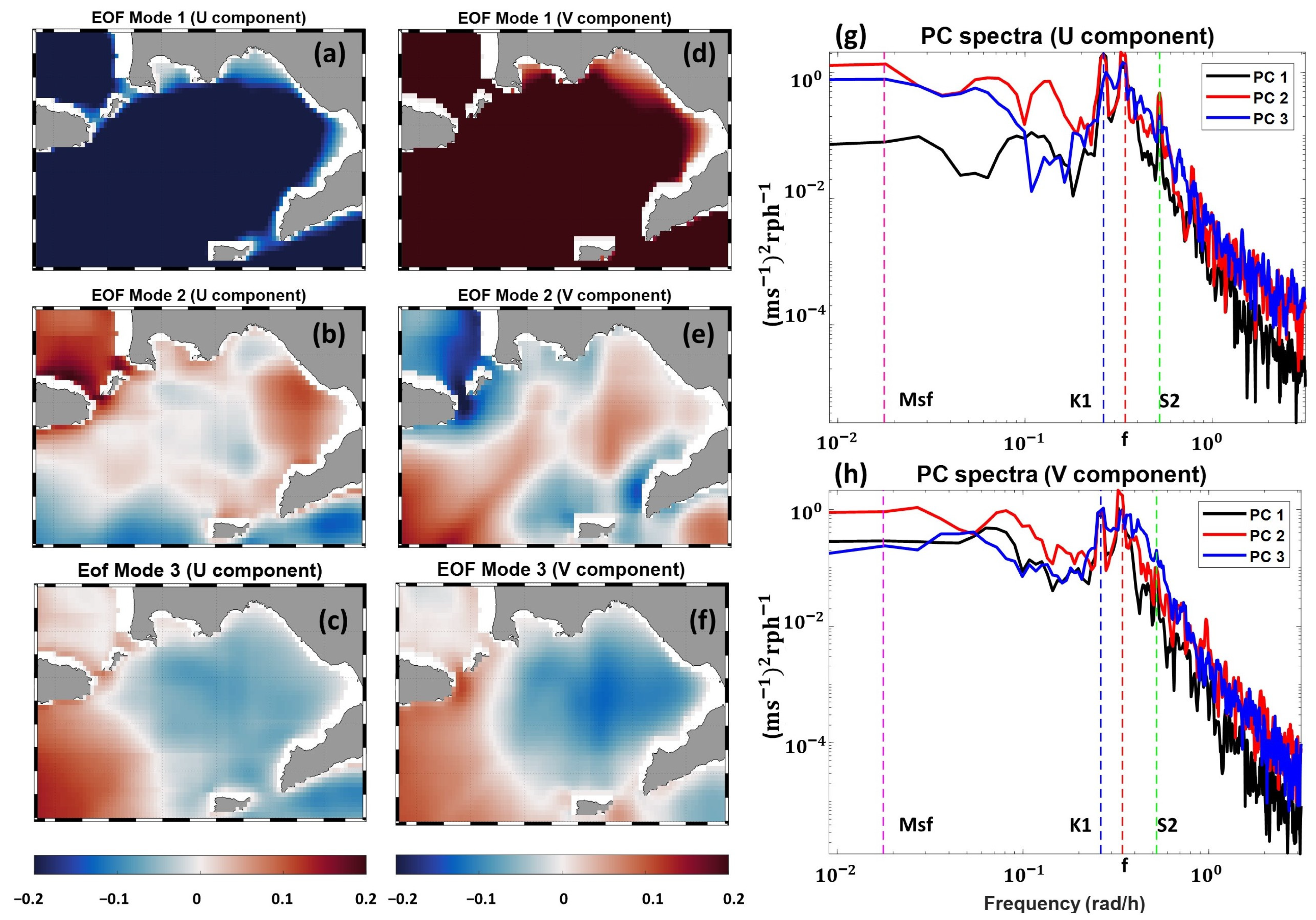
Mode Number	Explained Variance (%) U Component	Cum. Variance (%) U Component	Explained Variance (%) V Component	Cum. Variance (%) V Component
Mode 1	34.9	34.9	22	22
Mode 2	18.5	53.5	20.9	43
Mode 3	10.4	63.8	10.5	53.5
Mode 4	5.6	69.5	7.1	60.7

lists the percentage of variance explained by the first four modes together with the cumulative percentage of variance.

EOF Mode 1 accounted for 34.9% (22%) of the total variance, while 18.5% (20.9%) of the total variance is explained by EOF Mode 2 for the zonal (meridional) component. The first two modes account for 53.5% (43%) of the total variance. Mode 3 and Mode 4 together explain about 16% (17.7%) of the total variance. All four modes explain approximately 69.5% (60.7%) of the current variance, as shown in Table 7. In agreement with North’s rule of thumb [46], only the first four EOF modes (five modes) for the zonal (meridional) component are significant. Here we focused on the first three modes.

The spatial pattern of EOF Mode 1 (black dashed line in Figure 7a,b) suggests northeastward flow for the first 11.90 m depth. Beyond this depth, the flow is southeastward, suggesting a rotation of the flow field. The spectral analysis associated with the first principal component (Figure 7c,d) shows peaks in the diurnal and semidiurnal bands as well as in the inertial band, highlighting the strong influence of the wind on the current field. The presence of inertial motions has to be accounted for the occurrence, as highlighted in Section 3.1, of perturbations in the BN area. In addition, low-frequency contributions are observed around 60 h, 90 h and 165 h for the zonal component and 55 h and 78 h for the meridional component. The spatial pattern of Mode 2 (red dashed line in Figure 7a,b) shows greater spatial variability, with northwesterly rotation and minimum amplitude of the current field at 8.90 m depth. Again, the diurnal peak is clearly shown in the spectral band (Figure 7d–g), but this time no significant peaks emerge in the local inertial frequency. Low-frequency contributions are observed around 60 h, 123 h and 330 h for the zonal component and 42 h and 130 h for the meridional component. The spatial pattern of Mode 3 (blue dashed line in Figure 7a,b) shows strong variability: the amplitudes presented two minima in the water column and the phase changed rapidly at the depths of minimum amplitudes. The spectral analysis performed on the principal component detects a strong contribution in the diurnal band mainly for the zonal component (Figure 7e) and a clear signal in the inertial band, especially in the meridional component (Figure 7h). Low-frequency contributions are observed around 60 h.

3.5. Sea Current Response to Wind Forcing

As the analysis of the rotational spectra and EOF has already shown, the influence of wind is evident in the surface layer of the water column.

Thus, before going into the details of the model data analysis (reported in Section 4), we seek to understand how observed marine dynamics respond to wind forcing and to the water column depth where the wind signal is prominent.

For this purpose, we computed the complex lagged cross-correlation function (Kundu, 1976) between the wind stress and the sea current time series in seven ADCP bins from the surface to the bottom, following a similar approach adopted in [47,48]. The phase angle represents the average veering angle between the two vector time series. As mentioned in Section 2.3, to eliminate tidal and other sub-inertial oscillations, the vector time series were low-pass filtered by applying a digital symmetric low-pass filter (PL33).

Table 8. Lagged vector correlation between low-passed wind stress and low-passed currents. Amplitude and angular offset of lagged correlation between low-passed wind stress and observed low-passed currents.

Bin	Depth (m)	Zero-Lag Corr	Zero-Lag Veering (°)	Lag Max Corr (h)	Max-Lag Corr	Max-Lag Veer (°)
30	1.4	0.8	15.7	1	0.8	14.9
25	3.9	0.3	60.2	10	0.4	49.7
20	6.4	0.1	15.8	17	0.4	44.1
15	8.9	0.05	−75.8	20	0.2	46.5
10	11.4	0.2	−108.7	0	0.2	−108.7
5	13.9	0.2	−96.1	0	0.2	−96.1
1	15.9	0.3	−104.8	0	0.3	−104.8

summarizes, for each ADCP bin, the results of the analysis. A positive angle indicates that wind is rotated positively (counterclockwise) compared to the current. The response to wind stress at the surface was almost immediate since correlation was maximized at 1 h lag with about 15^° veering to the left of the wind stress vector. As pointed out in [49], the wind-driven flow is isotropic in the open sea, but horizontal pressure gradients and the friction acting over the bottom topography could considerably increase the complexity of its behavior [50,51]. As assessed in [52], the response of the surface current could also be anisotropic and asymmetric in our case, as the local effects of topography and the frictional balance with wind are not equivalent in the zonal and meridional directions. The lag of the maximum correlation with the wind stress vector constantly increased along the water column, reaching 20 h at 9 m depth, with currents to the left of the wind stress vector. Below this depth, the veering angles were negative, meaning that currents were pointing to the right of the wind stress vector.

3.6. Comparison between Modeled and Observed Wind Stress

Due to the significance of the local forcing on the structure of the sea current field in the BN, especially in the near-surface layer, we briefly compare the Skyron wind stress data used to force the CROM model with the wind stress recorded by the MEDA B Napoli. This comparison helped us to interpret the potential differences we identify from the outcomes of the modeled hindcasts and of the observed time series.

The Skyron wind stress time series was obtained by spatial averaging of the hourly values over 37 grid points (see Figure 8), and the comparison was performed on the overlapping portion of the time series. The correlations were applied for the hourly original (unfiltered) data, and for the time series after the removal of tides and other sub-inertial oscillations (PL-33 low-pass filtered time series). The 95% confidence bound is 0.08 for the April wind stress dataset and 0.09 for May. The qualitative comparison between the Skyron winds stress and the observed wind stress shows an underestimation of the simulated wind stress compared to the observed one. Overall, the Skyron wind stress is estimated to be about 15% (13% for April and 16% for May) of the observed one. On the other hand, the proximity to the coast of our study area has to be considered, as we expect that local factors strongly affect the meteorological model response. The resulting correlation coefficients are shown in

Table 9. Correlation coefficient between filtered and unfiltered observed and modeled wind stress in April and May 2016.

CC	April (Unfiltered)	April (Filtered)	May (Unfiltered)	May (Filtered)
U	0.64	0.88	0.13	0.27
V	0.51	0.78	0.07	−0.02

. Both vector correlation coefficients were significantly higher for the filtered series, apart from the meridional component in May. However, while the obtained correlation coefficients reveal a strong significant relationship between the model and the observations for the April time series, this is not the case for May, where the correlation is not statistically significant.

The above results suggest that the simulated current field for April was more accurate than that for May since for this last case the response is biased by the poor accuracy of the simulated wind field. In addition, given the lower intensity of the simulated wind stress, we expect a weaker surface simulated current field response compared to the observed ones.

4. Model Data Analysis

4.1. Model Marine Hydrology

The hydrological vertical profiles (T, S and $\mathsf{\rho }$ in a 70 m water column) observed at the LTER-MC sampling site have been compared with those simulated by CROM. The simulated vertical profiles are averaged over 37 grid points in the area defined in Figure 8. Simulation data are provided on 40 sigma levels; thus, to make the measurements comparable, linear interpolation on equidistant zeta levels (vertical resolution of 1 m) was performed. In addition, through the computation of the percentage error (E%), we are able to identify the depth at which we record the maximum difference between the observed and simulated datasets. The sign is kept to highlight the model over/underestimation.

The Taylor diagrams of Figure 8 summarize the statistical features (the Pearson correlation coefficient, the root-mean-square error (RMSE) and the standard deviation) of the modeled (point B in Figure 8) and observed (point A in Figure 8) hydrological dataset. The Pearson correlation coefficient is related to the azimuthal angle (blue contours in Figure 8); the centered RMSE in the simulated data is proportional to the distance from the point on the x-axis identified as “observed” (green contours in Figure 8); the standard deviation of the simulated pattern is proportional to the radial distance from the origin (black contours in Figure 8). It is evident from these diagrams that the distances of model results from the observations are fairly small for T and ρ (this means good agreement between the simulated and observed data), while the salinity shows greater differences between simulated and observed datasets. Regarding the freshwater contributions, as discussed in [53], the lack of data is a recurring problem in the Mediterranean Sea and hampers the study of water resources at the relevant scale [54,55]. Few estimates are available for long-term water discharge into the Mediterranean Sea, which is characterized by a wide range of variability. As far as the water mass exchanges of the Tyrrhenian Sea with the Mediterranean Sea are concerned, please refer to the recent review [6]. Moreover, refer to [56], in which the authors developed a detailed study of the impact of the freshwater inflow from the Volturno river on the coastal circulation. Finally, in [16], the authors studied the role played by wind stress and anomalous freshwater runoff in the formation and evolution of the filaments that originate on the shelf, which transport nutrient-rich, polluted waters directly offshore or into the GN.

Considering these statistical features, and from the analysis of the vertical profiles (Figure 9a–c), we observe that the model is able to reproduce the hydrology along the water column. Overall, the simulated temperature presents values lower than the LTER-MC-measured ones (Figure 9a) for the total survey period. The maximum temperature difference is recorded in June (see

Table 10. Maximum error difference between observed and simulated hydrological data.

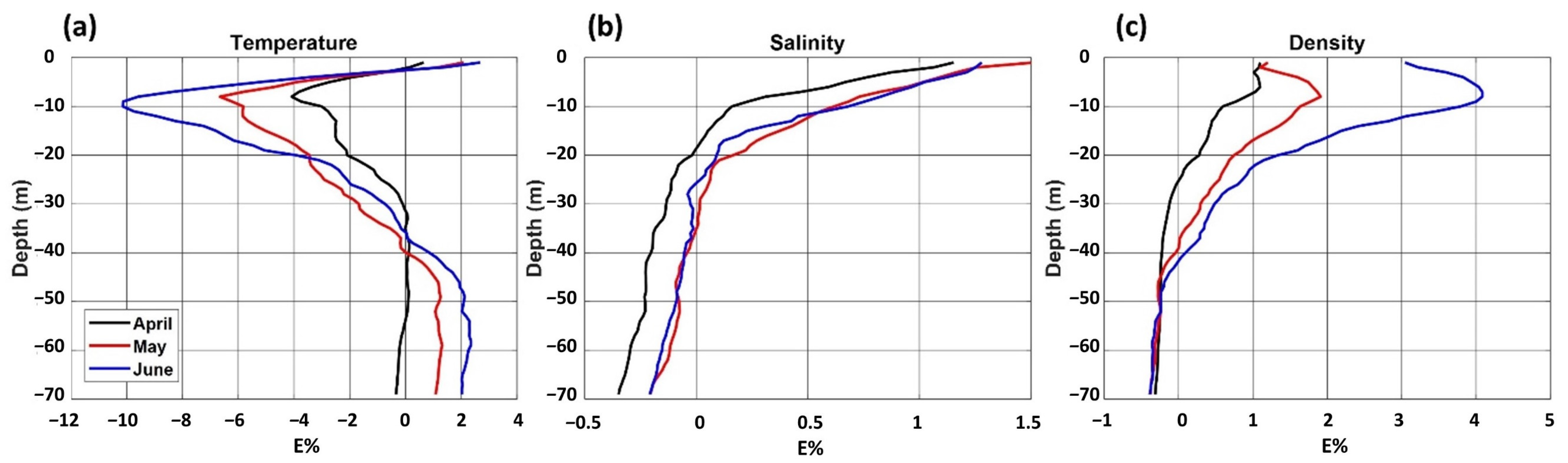
E%	Depth of Max E% (m)	Temperature	Depth of Max E% (m)	Salinity	Depth of Max E% (m)	Density
April	8	−4.08	1	1.15	1	1.09
May	8	−6.65	1	1.51	8	1.90
June	10	−10.13	1	1.27	8	4.08

and Figure 10a) near the 10 m depth. In this case, the model underestimates the temperature value recorded by about 10%.

In the simulated vertical salinity profiles (see dashed line in Figure 9b), there is no stratification, and the observed halocline (in the first 20 m of depth) does not appear. Thus, in the surface layer, the simulated salinity appears slightly higher than that actually observed, while below 20 m depth we observe good agreement between the numerical results and the observations (Figure 9b). In May, we found the maximum difference (Table 10 and Figure 10b) at 1 m depth. The disagreement in the first 20 m is mainly due to the lack of river inputs and possible sources of freshwater discharges from the coast in the numerical simulations. As already highlighted in the comment on the Hovmöller diagrams of Figure 2a, the freshwater inputs at the LTER-MC sampling site reduce the sea surface salinity with the resulting stratification of the water column (Figure 9b).

As a result, the simulated density is in good agreement with observations in the sub-surface layer (below 20 m depth, see Figure 9c) due to the simulated salinity and temperature features described above. The maximum density difference is recorded in June (see Table 10 and Figure 10c) at a depth of about 8 m.

In Figure 11, we compare the monthly mean hydrological parameters observed and simulated in the first 10 m depth and in the remaining 60 m. Following [32], we also evaluate the mixed layer depth (MLD) defined as the thickness of the layer within which the density anomaly interval was ≤0.05 kg m⁻³, both for the observed and simulated dataset. For further methods to estimate the MLD, see [57].

The MLD is one of the most important quantities in the upper ocean because it defines the quasi-homogeneous surface region of density that directly interacts with the atmosphere [58], and therefore the correct reproduction of MLD is essential for several aspects; it is primarily determined by a balance between the turbulent mixing caused by wind stress and heat exchange at the air–sea interface. This region also plays a central role in long-term climate and weather, as well as in the oceanic food chain (for its link with the primary production of phytoplankton biomass), and its seasonal variability is a prime factor in the air–sea exchange [59].

In both cases, we observe (values are shown in

Table 11. MLD observed and simulated by CROM.

Mixed Layer Depth (m)	April	May	June
LTER-MC	2.05	1.57	2.99
CROM	2.14	1.86	1.70

) very low MLD, with observed (simulated) values around 2.05 m (2.14 m) for April, 1.57 m (1.86 m) for May and 2.99 m (1.70 m) for June. Since the MLD computation is based on the density anomaly, it is worth noting that the largest deviation is in June because the maximum difference between the observed and simulated density profiles is found. As pointed out in [60], as the MLD becomes shallower in the spring, phytoplankton photosynthetic rates increase in response to the increasing availability of daily irradiance.

4.2. Mean Surface Current Field

We then proceed with the description of the simulated monthly mean surface current at the basin scale (not shown). Similar features emerge in the three months. Overall, the northwestern Tyrrhenian stream drives an anticyclonic circulation in the GN, with currents entering the basin through the Bocca Piccola opening (between the Sorrento peninsula and the island of Capri) from the Gulf of Salerno and through the Bocca Grande opening (between Capri and the island of Ischia). Near Capri Island, the presence of an anticyclonic structure emerges (which persists also in the months of May and June), influenced by the northwestern Tyrrhenian stream and by the southeastern currents that border Ischia Island, heading towards the interior of the Gulf.

4.3. Basic Statistics of Simulated Surface Current in the BN

We now briefly discuss the statistical results obtained with reference to the simulated spatially averaged surface current dataset in the BN.

Table 12. Basic statistical properties of surface simulated zonal (u) and meridional (v) currents for the April–June period.

	Max (cm/s)	Min (cm/s)	Mean (cm/s)	Median (cm/s)	Std (cm/s)	RMS (cm/s)
April (u)	12.6	−5.9	2.5	2.1	2.8	3.8
May (u)	12.2	−3.6	1.7	1.6	2.4	2.8
June (u)	22.1	−8.5	1.7	1.5	2.6	3.1
April (v)	9.9	−7.8	1.4	1.4	2.3	2.7
May (v)	7.1	−6.2	0.8	1.1	2.1	2.2
June (v)	21.3	−8	1.1	1.2	2.5	2.8

summarizes the basic statistical properties for the hourly time series of the u (east–west) and v (north–south) current components for April, May and June 2016. Here we considered only the SSC field. The absolute value of the u component amplitudes did not exceed 23 cm/s in the east direction and 9 cm/s in the west direction; for the v component, maximum values did not exceed 22 cm/s in the north direction, and maximum values in the south direction were below 9 cm/s. Mean and median values were both low and positive; thus, the time-averaged flow had a northeastward component, in accordance with the observed data. However, the simulated surface current field is weaker than that observed due to the lower modeled wind stress intensity used to force CROM.

4.4. SSC Frequency and Tidal Analysis

Following the approach adopted in Section 3.3, we now provide the results obtained by considering the rotary spectra and harmonic analysis applied to the spatially averaged current field in the BN area (see Figure 8l). Figure 12 shows the main clockwise and counterclockwise spectra of the CROM-simulated surface current field and Skyron wind stress.

Again, the tidal diurnal frequency band (K1, blue vertical dashed line), the tidal semidiurnal frequency band (S2, green vertical dashed line), the local inertial frequency band (f = 0.3432 rad/h, red vertical dashed line) and the low-frequency band (Msf, violet vertical dashed line) are evidenced in the sea current (Figure 12a–c) and wind stress (Figure 12d–f) rotary spectra. The current variance appeared to be larger in the CW (negative) spectrum than the CCW (positive) portion for the diurnal frequency band both for sea surface current and wind stress as highlighted for the observed data, suggesting an anticyclonic rotation of the surface current fields in the area. In this case, a significant signal in the long-term, low-frequency tidal band was also detected in April surface and wind stress spectra. As for the observed dataset, the ellipses for K1 currents in the upper layer are much larger than those for other tidal constituents.

However, some differences appear if we compare these results with those reported in Section 3.4. Firstly, the energy content of the simulated surface current field throughout the investigation period is lower than the observed one. This can be explained by the low intensity of the simulated wind stress and the consequently weaker response of the surface current field. Moreover, although no significant contribution in the inertial frequency band is found in the observed spectra, this is evident in the simulated surface current spectra over the entire investigation period mainly in the clockwise part of the spectrum.

Table 13. Tidal ellipse parameters (major and minor axes, inclination and phase) together with 95% confidence levels (Emaj, Emin, Einc, Epha) for the tidal constituents with SNR greater than 2. (a), (b) and (c) refer to surface current in April, May and June, respectively. (d), (e) and (f) refer to wind stress for April, May and June.

Tide (a)	Freq (cph)	Major (cm/s)	Emaj (cm/s)	Minor (cm/s)	Emin (cm/s)	Inc (°E)	Einc (°E)	Pha	Epha	Snr
MSF	0.0028219	0.9	0.4	0.6	0.3	152.7	45.2	355.4	52.1	4
K1	0.0417807	1.6	0.5	−1	0.3	4.2	23.9	301.9	29.8	12
S2	0.0833333	0.4	0.3	−0.2	0.3	54.9	64.1	278.6	67.8	2.1
(b)
K1	0.0417807	1.2	0.4	−0.8	0.6	170.7	69.2	300.1	56.4	6.3
S2	0.0833333	0.4	0.2	−0.3	0.2	37.7	83	301.8	76.9	2.9
(c)
K1	0.0417807	1.6	0.7	−1.2	0.7	178.2	70.2	213.1	73.6	5
(d)	Freq (cph)	Major (N/m2)	Emaj (N/m2)	Minor (N/m2)	Emin (N/m2)	Inc (°E)	Einc (°E)	Pha	Epha	Snr
MSF	0.0028219	0.011	0.002	0.005	0	29.4	12.9	190.7	13.4	39
K1	0.0417807	0.007	0.003	−0.003	0	37.5	31.6	312.3	33.1	5.6
(e)
S2	0.0833333	0.002	0.001	−0.001	0	55.9	65.2	255	67.2	2.7
(f)
K1	0.04178070	0.005	0.002	−0.002	0	32.7	50.1	52.4	41.1	5.2
S2	0.08333333	0.003	0.001	−0.001	0	39.9	49.4	73.6	42.6	3.6

shows the ellipse parameters for the tidal constituents with SNR greater than 2 for both the simulated surface current field and the wind stress data.

4.5. SSC Skill Score

To understand the ability of the CROM model to simulate coastal dynamics in the very small area defined in Figure 10, whose linear dimension is comparable to the horizontal grid steps, the model skill score (d) proposed in [61] will be analyzed. As stated by Willmot [61], this descriptive statistic reflects the degree to which the observed variate is accurately estimated by the simulated variate. It varies between 0 (complete disagreement) and 1 (perfect agreement). Some authors [62] suggest the inclusion of relative error measures (e.g., this model skill score) and one absolute error measure (e.g., RMSE) to assess the model performance [49].

$$\mathrm{d}=1-\frac{\sum |{\mathrm{X}}_{\mathrm{model} }-{\mathrm{X}}_{\mathrm{obs}}{|}^2}{\sum {(|{\mathrm{X}}_{\mathrm{model}}-{ \overline{\mathrm{X}} }_{\mathrm{obs}}|+\left|{\mathrm{X}}_{\mathrm{obs}}-{ \overline{\mathrm{X}} }_{\mathrm{obs}}\right|)}^2}$$

(3)

Table 14. Model skill score and RMSE between simulated and observed sea surface currents.

(a)	d (u)	RMSE (u)	d (v)	RMSE (v)
April	0.53	6.2 cm/s	0.42	8 cm/s
May	0.38	7.1 cm/s	0.39	8.7 cm/s
June	0.34	7.1 cm/s	0.40	8.7 cm/s
(b)	d (u)	RMSE (u)	d (v)	RMSE (v)
April	0.64	3.5 cm/s	0.50	5.3 cm/s
May	0.51	3.5 cm/s	0.44	5.4 cm/s
June	0.37	3.6 cm/s	0.44	5.4 cm/s

shows the model skill score (d) and the RMSE computed with regard to the unfiltered (panel a) and low-pass filtered (panel b) zonal and meridional components (1 h sampling rate) of the surface current field recorded by the ADCP and simulated by the CROM model in the area defined in Figure 8 for April, May and June 2016.

Table 14 shows that the maximum d for the zonal component occurs in April. In general, there is an overall increase in the skill score and a decrease in RMSE taking into account the low-pass filtered signals. The increase is remarkable for April, where we observe a skill score of 0.64 for the low-pass filtered time series of the zonal component. Considering that, as highlighted in Section 3.6, the Skyron wind stress is more accurate for April than for May, we conclude that the agreement and, on the other hand, the disagreement that emerge from the skill computation definitely depend on the accuracy of the adopted wind. In addition to the differences related to the wind forcing, another fundamental reason for the discrepancy between the model output and the observed dataset has to do with the horizontal resolution. The CROM model, despite its high spatial resolution, cannot satisfactorily simulate the circulation in the small area under investigation, which is, in addition, close to the coasts, so the simulated currents are particularly sensitive to the lateral boundary conditions.

4.6. BN and Basin-Scale EOF Modes

In this section, we will discuss the EOF results by considering the simulated sea current data. First, the analysis will be carried out on the spatially averaged sea current time series in the 37 grid points (shown in Figure 8l) for the first 16 m of depth in order to compare the simulated dynamics in the BN area with those recorded by the ADCP probe. We will then focus on the analysis of the larger-scale features by applying the EOF to the surface current field simulated by CROM over the whole basin.

Regarding the BN, the results of our analysis are presented in Figure 13. Here we show the spatial pattern for the first three EOF modes of the zonal (Figure 13a) and meridional (Figure 13b) components, and the frequency spectra of the associated principal components (Figure 13c–h).

In this case, the EOF Mode 1 accounted for 84.81% (70.98%) of the total variance, while 13.40% (22.49%) of the total variance is explained by EOF Mode 2 for the zonal (meridional component). The first two modes account for 98,21% (93.47%) of the total variance. Mode 3 of the zonal (meridional) component explains only 1.31% (5.67%) of the total variance and is not statistically significant following North’s rule of thumb [46].

The spatial pattern of the EOF Mode 1 (black dashed line in Figure 13) suggests northeastward flow for the whole depth, with greater variability in the near-surface layer. The spectral analysis associated with the first principal component (Figure 13c–f) shows peaks in the diurnal period and a sharp peak in the local inertial band. In this case, the inertial component is far more significant than that in the observed data, becoming the main feature of the spectrum. The spatial pattern of the second mode (red dashed line in Figure 13a,b) shows greater spatial variability, with southwesterly rotation and minimum amplitude of the current field at 8.50 m depth. Again, the inertial peak is clearly shown in the spectral band (Figure 13d–g), but this time no significant peaks emerge in the diurnal and semidiurnal bands. The spatial pattern of Mode 3 (blue dashed line in Figure 13a,b) shows strong variability, according to the observed data: the amplitudes presented two minima in the water column and the phase changed rapidly at the depths of minimum amplitudes. Again, the spectral analysis performed on the principal component detects a strong contribution in the inertial band both for the zonal and meridional components (Figure 13e–h) and also a clear peak in the diurnal band.

Let us now analyze the main three EOF modes of the model-simulated surface current field for April, May and June 2016. In addition, the frequency spectra for the expansion coefficients associated with the first three modes are also reported. Figure 14 shows the spatial pattern for Mode 1 (which alone accounts for 84% of the variance), Mode 2 (which accounts for about 5% of the variance) and Mode 3 (which accounts for about 3% of the variance) for April 2016 both for the zonal (Figure 14a–c) and meridional (Figure 14d–f) components. The flow field for Mode 1, stronger near the Bocca Grande opening, is approximately spatially uniform and directed towards the northwest. On the other hand, Mode 2 shows greater variability, with a northeastward current field near the Bocca Grande opening and a southwestward flow in the inner part of the basin. Mode 3 shows a strong spatial variability, but the basin-scale current field is mainly directed towards the southeast.

The frequency behavior of the expansion coefficient associated with the three principal modes is shown in Figure 14g,h. A sharp, well-defined peak at the local inertial signal was still present in the spectrum for all three modes. Moreover, a clear peak in the diurnal band is also observed, but the contribution around the semidiurnal band is small.

Figure 15 shows the spatial pattern for Mode 1 (which alone accounts for 85% of the variance), Mode 2 (which accounts for about 6% of the variance) and Mode 3 (which accounts for about 2% of the variance) for May 2016 both for the zonal (Figure 15a–c) and meridional (Figure 15d–f) components. As for April, the flow field for Mode 1 is approximately spatially uniform and northwestward. Mode 2 suggests the presence of a large anticyclonic structure in the offshore area of the GN. In contrast, the third mode shows a northwesterly flow dominating the entire gulf. The frequency behavior of the expansion coefficient associated with the three principal components (Figure 15g,h) suggests that the inertial oscillations and the diurnal and semidiurnal tide dominate the energy content of the spectrum.

Figure 16 shows the vector field for Mode 1 (which alone accounts for 88% of the variance), Mode 2 (which accounts for about 3% of the variance) and Mode 3 (which accounts for about 2% of the variance) both for the zonal (Figure 16a–c) and meridional (Figure 16d–f) components for June 2016. Again, the flow field for Mode 1 is approximately spatially uniform and northwestward. The second mode highlights high spatial variability, while Mode 3 suggests the presence of a southwesterly structure in the GN. The frequency behavior of the expansion coefficient associated with the three principal components reveals a clear peak in the diurnal, inertial and semidiurnal frequency bands.

5. Conclusions

This investigation was aimed at understanding the marine dynamics in the GN through an integrated approach that involved the use of current and hydrological data simulated by a high-resolution coastal ocean model (CROM) and measurements acquired at two locations.

The qualitative and basic statistical analysis carried out on the data measured at the LTER-MC sampling site and at MEDA B Naples buoy allowed us to describe the dynamics affecting the BN during the spring period of 2016. Overall, the period was characterized by a stable forcing, apart from occasional events of notable intensity associated with the passage of depressional systems in the area.

The surface current field in the BN, typically directed toward the northeast, is significantly affected by the wind as it responds to it instantaneously and with significant correlation, as evidenced by the complex correlation coefficient analysis of Section 3.5. The surface current field deviates leftward from the wind direction. As assessed in [52], the response of the surface current could also be anisotropic and asymmetric in our case, as the local effects of topography and the frictional balance with wind are not equivalent in the zonal and meridional directions.

To identify the modes of variability and time scales of the flow as well as the periodicity in the local forcing, we used the rotary spectra analysis applied to the surface current field and the wind stress. The outcomes of this analysis again highlight the influence of the wind on the surface layer as suggested by the diurnal and semidiurnal peaks detected both in the wind stress and in the surface current rotary spectra, mainly due to the breeze regime. In addition, the energy content in the surface current rotary spectra is greater in the clockwise spectrum compared to the counterclockwise one, revealing an anticyclonic rotation of the current field in the BN. According to the harmonic analysis, tidal forcing was weak since astronomical tides explained only 19.3% of the wind stress variance for April and 16.2% for May, while explaining about 19.8% (April), 16.2% (May) and 26.1% (June) of the sea surface current, confirming what has been previously reported in the literature [2,4]. Moreover, even though the tides in the GN are mainly semidiurnal, as reported in [4], the diurnal peak dominates in the observed spectrum. However, the diurnal wind stress forcing related to the diurnal sea-breeze regime was found to increase the current variance at the K1 tidal diurnal frequency band [63].

On the other hand, the hydrological data analysis confirms that the study area is affected by lateral advection of freshwater that leads to a decrease in surface salinity, thus enhancing the water column stability, as reported in previous studies (e.g., [32]). In stratified conditions, low-salinity waters float at the surface, thereby enhancing the water column stability and reducing the mixed layer depth. The low mixed layer and developed thermocline (found in both the observed and the modeled hydrological data) of this period limit the current response to wind in the shallower layer of the water column. In addition, this hydrological condition promotes the occurrence of inertial phenomena [2,4,9], which are clearly displayed in the spectra of the simulated current field.

As previously pointed out, the presented results are depictive of the coastal circulation, as the performed analysis is limited by the sparsity of the observed data, the shortness of the study period, the lack of valuable information such as the river inputs and the low wind forcing resolution. Therefore, we are unable to effectively identify the local dynamical pattern (around 2 miles from the coast), as shown by the observed low skill scores. In this sense, the simulated dynamics around the observation site are only indicative. Instead, both the wind resolution and the model resolution are suitable for reproducing basin-scale dynamic features.

More specifically, from the analysis of hydrological and current model data, we are able to define two major causes of discrepancy between the model and observations.

First, the lack of river inputs and potential spill sources within the model set-up produces some mismatch between the observed and modeled hydrological profiles, as reported in Section 4.1. These differences are mainly evident in the simulated vertical salinity profiles where there is no stratification, and the observed halocline (in the first 20 m of depth) does not appear. Thus, in the surface layer, the simulated salinity appears slightly higher than that actually observed, while below 20 m depth we observe good agreement between the numerical results and the observations.

As a result, the simulated density is in good agreement with observations in the sub-surface layer (below 20 m depth) due to the simulated salinity and temperature features described in Section 4.1. Unfortunately, for the investigation period, there are no river flow data available, or measurements that can be used to quantify the freshwater input due to spillage phenomena, and therefore we are unable to verify whether, with a more accurate set-up, the model would be able to better respond from the hydrological point of view, apart from its resolution.

Secondly, given the considerable influence of the local forcing on the surface current field, it is clear that the accuracy of the response of the simulated current field would depend on the accuracy of the wind stress used to force the model. Results of Section 3.6 reveal that the correlation coefficients between the modeled and the observed wind stress in the BN were significantly augmented for the low-pass filtered time series, apart from the meridional component in May. Moreover, while the obtained correlation coefficients reveal a strong significant relationship between the model and the observations for the April time series, this is not the case for May where the correlation is not statistically significant. As revealed by the skill score analysis of Section 4.5, in April, the model accurately simulates the surface current field in the study area, especially if we consider the filtered signals, while in May, the response is biased by the low accuracy of the modeled wind. In addition, as the statistical analysis shown in Section 4.3 suggests, the response of the simulated surface current field is weaker than the observed response, and this is a direct consequence of the low-intensity wind stress used to force the model. The Skyron data used for the evaluation of surface stresses may lack the necessary resolution to describe accurately the nearshore areas, where variations in land topography could strongly affect the winds, leading to an underestimation of the wind speeds. However, for the survey period, it is not possible to force the model with higher-resolution wind data, and on the other hand, given the lack of a basin-scale meteorological observational network, this cannot be done with observed wind data, since they are sampled at a single observational point.

Here it is worth highlighting that the building of a careful monitoring network in the GN, integrated with the results of numerical models, could certainly allow us to better understand the GN basin-scale dynamics.

The frequency analysis reported in Section 4.4, applied to both the simulated wind stress and the simulated surface current field, highlights some common features with the observed spectrum, such as the higher energy content of the clockwise spectrum compared to the counterclockwise one, proof of an anticyclonic motion in the area, and the presence of diurnal and semidiurnal peaks associated with the breeze regime. However, the dominant feature of the simulated current spectrum is the presence of a prominent energy-level peak in the frequency band corresponding to the local inertial frequency, a feature not so evident in the observed spectrum of Section 3.3. This also emerges from the spectra of the expansion coefficient associated with the third principal mode of the basin-scale EOF analysis where a sharp, well-defined peak at the local inertial signal was still present in the CW spectrum. We point out, however, that the inertial component is also detected by the EOF analysis applied to the observed data (reported in Section 3.5), but that it is not as strong as that in model data. In the case of the observed data, the close distance from the coast and the shallow depth of the seabed (with the resulting higher bottom friction) at the MEDA B Napoli location suppress the development of inertial motions by dissipating their energy, as reported in [64]. On the other hand, in the case of the model data, the depth of the chosen grid points is on average greater than the station depth, which means fewer friction phenomena, and this enhances the development of inertial motions.

As assessed in [2,9,17], inertial phenomena in the GN are more evident in the warmer period of the year, when the higher temperatures favor the evolution of a stable thermocline, while during winter, inertial events are by contrast less recurrent.

Moreover, the space-averaged Skyron wind stress time series in the BN area and the observed wind stress time series (not shown) clearly show the presence of a few strong wind stress events (associated with the passage of depressional systems as highlighted in Section 3.1) that break up the limited variability in both directional and wind intensity. Since the inertial currents are excited by impulsive wind stress, given the favorable hydrological features and considering that the breeze regime is not well developed as in the summer period, it is not surprising that the inertial component dominates the basin-scale dynamics during the 2016 spring.

References

- Carrada, G.C.; Hopkins, T.S.; Bonaduce, G.; Ianora, A.; Marino, D.; Modigh, M.; Ribera, D.M.; di Scotto, C.B. Variability in the Hydrographic and Biological Features of the Gulf of Naples. Mar. Ecol. 1980, 1, 105–120. [Google Scholar] [CrossRef]
- Menna, M.; Mercatini, A.; Uttieri, M.; Buonocore, B.; Zambianchi, E. Wintertime Transport Processes in the Gulf of Naples Investigated by HF Radar Measurements of Surface Currents. Nuovo Cim. C 2008, 30, 605–622. [Google Scholar] [CrossRef]
- Uttieri, M.; Cianelli, D.; Nardelli, B.B.; Buonocore, B.; Falco, P.; Colella, S.; Zambianchi, E. Multiplatform Observation of the Surface Circulation in the Gulf of Naples (Southern Tyrrhenian Sea). Ocean Dyn. 2011, 61, 779–796. [Google Scholar] [CrossRef]
- Cianelli, D.; Uttieri, M.; Buonocore, B.; Falco, P.; Zambardino, G.; Zambianchi, E. Dynamics of a Very Special Mediterranean Coastal Area: The Gulf of Naples. In Mediterranean Ecosystems: Dynamics, Management and Conservation; Nova Science Publishers: Hauppauge, NY, USA, 2012; pp. 129–150. ISBN 978-1-61209-146-4. [Google Scholar]
- Cianelli, D.; Falco, P.; Iermano, I.; Mozzillo, P.; Uttieri, M.; Buonocore, B.; Zambardino, G.; Zambianchi, E. Inshore/Offshore Water Exchange in the Gulf of Naples. J. Mar. Syst. 2015, 145, 37–52. [Google Scholar] [CrossRef]
- Iacono, R.; Napolitano, E.; Palma, M.; Sannino, G. The Tyrrhenian Sea Circulation: A Review of Recent Work. Sustainability 2021, 13, 6371. [Google Scholar] [CrossRef]
- Falco, P.; Buonocore, B.; Cianelli, D.; Luca, L.; Alberto, G.; Iermano, I.; Kalampokis, A.; Saviano, S.; Uttieri, M.; Zambardino, G.; et al. Dynamics and Sea State in the Gulf of Naples: Potential Use of High-Frequency Radar Data in an Operational Oceanographic Context. J. Oper. Oceanogr. 2016, 9, s33–s45. [Google Scholar] [CrossRef] [Green Version]
- Krauzig, N.; Falco, P.; Zambianchi, E. Contrasting Surface Warming of a Marginal Basin Due to Large-Scale Climatic Patterns and Local Forcing. Sci. Rep. 2020, 10, 17648. [Google Scholar] [CrossRef]
- Moretti, M.; Spezie, G.; Vultaggio, M. Sub-Inertial Waves Observed in the Gulf of Naples. Rapp. Comm. Int. Mer Medit. 1983, 28, 2. [Google Scholar]
- De Pippo, T.; Donadio, C.; Pennetta, M.; Petrosino, C.; Francesco, T.; Valente, A. Coastal Hazard Assessment and Mapping in Northern Campania, Italy. Geomorphology 2008, 97, 451–466. [Google Scholar] [CrossRef]
- Tornero, V.; Ribera d’Alcalà, M. Contamination by Hazardous Substances in the Gulf of Naples and Nearby Coastal Areas: A Review of Sources, Environmental Levels and Potential Impacts in the MSFD Perspective. Sci. Total Environ. 2014, 466–467, 820–840. [Google Scholar] [CrossRef]
- Mattei, G.; Rizzo, A.; Anfuso, G.; Aucelli, P.P.C.; Gracia, F.J. A Tool for Evaluating the Archaeological Heritage Vulnerability to Coastal Processes: The Case Study of Naples Gulf (Southern Italy). Ocean Coast. Manag. 2019, 179, 104876. [Google Scholar] [CrossRef]
- Gravili, D.; Napolitano, E.; Pierini, S. Barotropic Aspects of the Dynamics of the Gulf of Naples (Tyrrhenian Sea). Cont. Shelf Res. 2001, 21, 455–471. [Google Scholar] [CrossRef]
- Grieco, L.; Tremblay, L.-B.; Zambianchi, E. A Hybrid Approach to Transport Processes in the Gulf of Naples: An Application to Phytoplankton and Zooplankton Population Dynamics. Cont. Shelf Res. 2005, 25, 711–728. [Google Scholar] [CrossRef]
- De Ruggiero, P. A High-Resolution Ocean Circulation Model of the Gulf of Naples and Adjacent Areas. Nuovo Cim. C 2013, 36, 143–150. [Google Scholar]
- Iermano, I.; Liguori, G.; Iudicone, D.; Buongiorno Nardelli, B.; Colella, S.; Zingone, A.; Saggiomo, V.; Ribera d’Alcalà, M. Filament Formation and Evolution in Buoyant Coastal Waters: Observation and Modelling. Prog. Oceanogr. 2012, 106, 118–137. [Google Scholar] [CrossRef]
- De Ruggiero, P.; Ernesto, N.; Iacono, R.; Pierini, S. A High-Resolution Modelling Study of the Circulation along the Campania Coastal System, with a Special Focus on the Gulf of Naples. Cont. Shelf Res. 2016, 122, 85–101. [Google Scholar] [CrossRef]
- de Ruggiero, P.; Esposito, G.; Napolitano, E.; Iacono, R.; Pierini, S.; Zambianchi, E. Modelling the Marine Circulation of the Campania Coastal System (Tyrrhenian Sea) for the Year 2016: Analysis of the Dynamics. J. Mar. Syst. 2020, 210, 103388. [Google Scholar] [CrossRef]
- Montuori, A.; de Ruggiero, P.; Migliaccio, M.; Pierini, S.; Spezie, G. X-Band COSMO-SkyMed Wind Field Retrieval, with Application to Coastal Circulation Modeling. Ocean Sci. 2013, 9, 121–132. [Google Scholar] [CrossRef] [Green Version]
- De Ruggiero, P.; Napolitano, E.; Iacono, R.; Pierini, S.; Spezie, G. A Baroclinic Coastal Trapped Wave Event in the Gulf of Naples (Tyrrhenian Sea). Ocean Dyn. 2018, 68, 1683–1694. [Google Scholar] [CrossRef]
- Sandvik, A.D.; Skagseth, Ø.; Skogen, M.D. Model Validation: Issues Regarding Comparisons of Point Measurements and High-Resolution Modeling Results. Ocean Model. 2016, 106, 68–73. [Google Scholar] [CrossRef]
- Lacava, T.; Ciancia, E. Remote Sensing Applications in Coastal Areas. Sensors 2020, 20, 2673. [Google Scholar] [CrossRef] [PubMed]
- Cianelli, D.; Uttieri, M.; Guida, R.; Menna, M.; Buonocore, B.; Falco, P.; Zambardino, G.; Zambianchi, E. Land-Based Remote Sensing of Coastal Basins: Use of an HF Radar to Investigate Surface Dynamics and Transport Processes in the Gulf of Naples. In Remote Sensing: Techniques, Applications and Technologies; Nova Science Publishers: Hauppauge, NY, USA, 2013; pp. 1–30. ISBN 978-1-62417-140-6. [Google Scholar]
- Saviano, S.; De Leo, F.; Besio, G.; Zambianchi, E.; Uttieri, M. HF Radar Measurements of Surface Waves in the Gulf of Naples (Southeastern Tyrrhenian Sea): Comparison with Hindcast Results at Different Scales. Front. Mar. Sci. 2020, 7, 492. [Google Scholar] [CrossRef]
- Wilkin, J.; Zhang, W.; Cahill, B.; Chant, R. Integrating Coastal Models and Observations for Studies of Ocean Dynamics, Observing Systems and Forecasting. In Operational Oceanography in the 21st Century; Springer: Cham, Switzerland, 2011; pp. 487–512. ISBN 978-94-007-0331-5. [Google Scholar]
- Iermano, I.; Moore, A.M.; Zambianchi, E. Impacts of a 4-Dimensional Variational Data Assimilation in a Coastal Ocean Model of Southern Tyrrhenian Sea. J. Mar. Syst. 2016, 154, 157–171. [Google Scholar] [CrossRef]
- De Mey-Frémaux, P.; Ayoub, N.; Barth, A.; Brewin, B.; Charria, G.; Campuzano, F.; Ciavatta, S.; Cirano, M.; Edwards, C.; Federico, I.; et al. Model-Observations Synergy in the Coastal Ocean. Front. Mar. Sci. 2019, 6, 436. [Google Scholar] [CrossRef] [Green Version]
- Ponte, R.M.; Carson, M.; Cirano, M.; Domingues, C.M.; Jevrejeva, S.; Marcos, M.; Mitchum, G.; van de Wal, R.S.W.; Woodworth, P.L.; Ablain, M.; et al. Towards Comprehensive Observing and Modeling Systems for Monitoring and Predicting Regional to Coastal Sea Level. Front. Mar. Sci. 2019, 6, 437. [Google Scholar] [CrossRef] [Green Version]
- Song, Y.; Haidvogel, D. A Semi-Implicit Ocean Circulation Model Using a Generalized Topography-Following Coordinate System. J. Comput. Phys. 1994, 115, 228–244. [Google Scholar] [CrossRef]
- Iacono, R.; Napolitano, E.; Marullo, S.; Artale, V.; Vetrano, A. Seasonal Variability of the Tyrrhenian Sea Surface Geostrophic Circulation as Assessed by Altimeter Data. J. Phys. Oceanogr. 2013, 43, 1710–1732. [Google Scholar] [CrossRef]
- Zingone, A.; Casotti, R.; Ribera d’Alcala, M.; Scardi, M.; Marino, D. St-Martin’s Summer—The Case of an Autumn Phytoplankton Bloom in the Gulf of Naples (Mediterranean-Sea). J. Plankton Res. 1995, 17, 575–593. [Google Scholar] [CrossRef]
- D’Alcalà, M.R.; Conversano, F.; Corato, F.; Licandro, P.; Mangoni, O.; Marino, D.; Mazzocchi, M.G.; Modigh, M.; Montresor, M.; Nardella, M.; et al. Seasonal Patterns in Plankton Communities in a Pluriannual Time Series at a Coastal Mediterranean Site (Gulf of Naples): An Attempt to Discern Recurrences and Trends. Sci. Mar. 2004, 68, 65–83. [Google Scholar] [CrossRef] [Green Version]
- Mazzocchi, M.G.; Licandro, P.; Dubroca, L.; Di Capua, I.; Saggiomo, V. Zooplankton Associations in a Mediterranean Long-Term Time-Series. J. Plankton Res. 2011, 33, 1163–1181. [Google Scholar] [CrossRef] [Green Version]
- Zingone, A.; Dubroca, L.; Iudicone, D.; Margiotta, F.; Corato, F.; Ribera d’Alcalà, M.; Saggiomo, V.; Sarno, D. Coastal Phytoplankton Do Not Rest in Winter. Estuaries Coasts 2010, 33, 342–361. [Google Scholar] [CrossRef]
- Blumberg, A.F.; Mellor, G.L. A Description of a Three-Dimensional Coastal Ocean Circulation Model. In Three-Dimensional Coastal Ocean Models; American Geophysical Union (AGU): Washington, DC, USA, 1987; pp. 1–16. ISBN 978-1-118-66504-6. [Google Scholar]
- Madec, G. NEMO Ocean Engine; NEMO System Team, Scientific Notes of Climate Modelling Center; Institut Pierre-Simon Laplace (IPSL): Guyancourt, France, 2017; Volume 27, ISSN 1288-1619. [Google Scholar] [CrossRef]
- Oddo, P.; Adani, M.; Pinardi, N.; Fratianni, C.; Tonani, M.; Pettenuzzo, D. A Nested Atlantic-Mediterranean Sea General Circulation Model for Operational Forecasting. Ocean Sci. 2009, 5, 461–473. [Google Scholar] [CrossRef] [Green Version]
- Napolitano, E.; Iacono, R.; Marullo, S. The 2009 Surface and Intermediate Circulation of the Tyrrhenian Sea as Assessed by an Operational Model. In The Mediterranean Sea; American Geophysical Union (AGU): Washington, DC, USA, 2014; pp. 59–74. ISBN 978-1-118-84757-2. [Google Scholar]
- Gonella, J. A Rotary-Component Method for Analysing Meteorological and Oceanographic Vector Time Series. Deep Sea Res. Oceanogr. Abstr. 1972, 19, 833–846. [Google Scholar] [CrossRef]
- Mooers, C.N.K. A Technique for the Cross Spectrum Analysis of Pairs of Complex-Valued Time Series, with Emphasis on Properties of Polarized Components and Rotational Invariants. Deep Sea Res. Oceanogr. Abstr. 1973, 20, 1129–1141. [Google Scholar] [CrossRef]
- Smith, S.D. Wind Stress and Heat Flux over the Ocean in Gale Force Winds. J. Phys. Oceanogr. 1980, 10, 709–726. [Google Scholar] [CrossRef]
- Pawlowicz, R.; Beardsley, B.; Lentz, S. Classical Tidal Harmonic Analysis Including Error Estimates in MATLAB Using T_TIDE. Comput. Geosci. 2002, 28, 929–937. [Google Scholar] [CrossRef]
- Kundu, P.K.; Allen, J.S. Some Three-Dimensional Characteristics of Low-Frequency Current Fluctuations near the Oregon Coast. J. Phys. Oceanogr. 1976, 6, 181–199. [Google Scholar] [CrossRef]
- Ghaffari, P. Acoustic Doppler Current Profiler Observations in the Southern Caspian Sea: Shelf Currents and Flow Field off Feridoonkenar Bay, Iran. Ocean Sci. OS 2010, 6, 737–748. [Google Scholar] [CrossRef] [Green Version]
- Imamura, J.; Takagi, K.; Nagaya, S.; Shimizu, M. Comparison of ADCP Measurements to Kuroshio Current Flow Simulations for Ocean Current Turbines. Proc. Inst. Mech. Eng. Part M J. Eng. Marit. Environ. 2022, 236, 174–184. [Google Scholar] [CrossRef]
- North, G.R.; Bell, T.L.; Cahalan, R.F.; Moeng, F.J. Sampling Errors in the Estimation of Empirical Orthogonal Functions. Mon. Weather Rev. 1982, 110, 699–706. [Google Scholar] [CrossRef]
- Cosoli, S.; Gacic, M.; Mazzoldi, A. Variability of Currents in Front of the Venice Lagoon, Northern Adriatic Sea. Ann. Geophys. 2008, 26, 731–746. [Google Scholar] [CrossRef]
- Cosoli, S.; Gacic, M. Comparison between HF Radar Current Data and Moored ADCP Currentmeter. Nuovo Cimento 2005, 28C, 865–879. [Google Scholar] [CrossRef]
- O’Donncha, F.; Hartnett, M.; Nash, S.; Ren, L.; Ragnoli, E. Characterizing Observed Circulation Patterns within a Bay Using HF Radar and Numerical Model Simulations. J. Mar. Syst. 2015, 142, 96–110. [Google Scholar] [CrossRef]
- Rabinovich, A.B.; Shevchenko, G.V.; Thomson, R.E. Sea Ice and Current Response to the Wind: A Vector Regressional Analysis Approach. J. Atmospheric Ocean. Technol. 2007, 24, 1086–1101. [Google Scholar] [CrossRef]
- Kim, S.Y.; Cornuelle, B.D.; Terrill, E.J. Anisotropic Response of Surface Currents to the Wind in a Coastal Region. J. Phys. Oceanogr. 2009, 39, 1512–1533. [Google Scholar] [CrossRef] [Green Version]
- Kim, S.Y.; Terrill, E.J.; Cornuelle, B.D.; Jones, B.; Washburn, L.; Moline, M.A.; Paduan, J.D.; Garfield, N.; Largier, J.L.; Crawford, G.; et al. Mapping the U.S. West Coast Surface Circulation: A Multiyear Analysis of High-Frequency Radar Observations. J. Geophys. Res. Oceans 2011, 116. [Google Scholar] [CrossRef] [Green Version]
- Bouraoui, F.; Grizzetti, B.; Aloe, A. Estimation of Water Fluxes into the Mediterranean Sea. J. Geophys. Res. Atmospheres 2010, 115. [Google Scholar] [CrossRef]
- Cudennec, C.; Leduc, C.; Koutsoyiannis, D. Dryland Hydrology in Mediterranean Regions—A Review. Hydrol. Sci. J. 2007, 52, 1077–1087. [Google Scholar] [CrossRef]
- Sivapalan, M.; Takeuchi, K.; Franks, S.W.; Gupta, V.K.; Karambiri, H.; Lakshmi, V.; Liang, X.; Mcdonnell, J.J.; Mendiondo, E.M.; O’connell, P.E.; et al. IAHS Decade on Predictions in Ungauged Basins (PUB), 2003–2012: Shaping an Exciting Future for the Hydrological Sciences. Hydrol. Sci. J. 2003, 48, 857–880. [Google Scholar] [CrossRef] [Green Version]
- Sorgente, R.; Di Maio, A.; Pessini, F.; Ribotti, A.; Bonomo, S.; Perilli, A.; Alberico, I.; Lirer, F.; Cascella, A.; Ferraro, L. Impact of Freshwater Inflow From the Volturno River on Coastal Circulation. Front. Mar. Sci. 2020, 7, 293. [Google Scholar] [CrossRef]
- Rivetti, I.; Boero, F.; Fraschetti, S.; Zambianchi, E.; Lionello, P. Anomalies of the Upper Water Column in the Mediterranean Sea. Glob. Planet. Change 2017, 151, 68–79. [Google Scholar] [CrossRef]
- Kara, A.B.; Rochford, P.A.; Hurlburt, H.E. Mixed Layer Depth Variability over the Global Ocean. J. Geophys. Res. Oceans 2003, 108. [Google Scholar] [CrossRef] [Green Version]
- Kantha, L.; Clayson, C. Small Scale Processes in Geophysical Fluid Flows; Elsevier: Amsterdam, The Netherlands, 2000; Volume 67, ISBN 978-0-12-434070-1. [Google Scholar]
- Diaz, B.P.; Knowles, B.; Johns, C.T.; Laber, C.P.; Bondoc, K.G.V.; Haramaty, L.; Natale, F.; Harvey, E.L.; Kramer, S.J.; Bolaños, L.M.; et al. Seasonal Mixed Layer Depth Shapes Phytoplankton Physiology, Viral Production, and Accumulation in the North Atlantic. Nat. Commun. 2021, 12, 6634. [Google Scholar] [CrossRef]
- Willmott, C.J. On the Validation of Models. Phys. Geogr. 1981, 2, 184–194. [Google Scholar] [CrossRef]
- Legates, D.; Mccabe, G. Evaluating the Use Of “Goodness-of-Fit” Measures in Hydrologic and Hydroclimatic Model Validation. Water Resour. Res. 1999, 35, 233–241. [Google Scholar] [CrossRef]
- Rosenfeld, L.K. Diurnal Period Wind Stress and Current Fluctuations over the Continental Shelf off Northern California. J. Geophys. Res. Oceans 1988, 93, 2257–2276. [Google Scholar] [CrossRef]
- Chen, S.; Chen, D.; Xing, J. A Study on Some Basic Features of Inertial Oscillations and Near-Inertial Internal Waves. Ocean Sci. 2017, 13, 829–836. [Google Scholar] [CrossRef]