Research on the Deep Learning Technology in the Hull Form Optimization Problem

Abstract

A high−accuracy objective function evaluation method is crucial in ship hull form optimization. This study proposes a novel approximate ship hull form optimization framework using the deep learning technology, deep belief network algorithm. To illustrate the advantages of using the deep belief network algorithm in the prediction of total resistance, two traditional surrogate models (ELMAN and RBF neural networks) are also employed in this study to predict total resistance for different modified ship models. It can be seen from the results that the deep belief network algorithm is more suitable for forecasting total resistance of a DTMB5512 ship model than the traditional surrogate models. Following this, two design variables are selected to alter the bow geometry of the DTMB5512 ship model. The total resistance for different modified ship hulls is estimated using the deep belief network algorithm. Furthermore, an optimal solution with minimum total resistance in a two−dimensional space is obtained using the particle swarm optimization algorithm. The optimization results indicate that the optimization framework using the deep belief network algorithm can obtain an optimal solution with the smallest total resistance for different ship speeds.

1. Introduction

The ship hull form optimization is one of the most important steps while designing a ship because an appropriate ship hull form is crucial for ensuring good hydrodynamic performance not only in calm water but also in waves. Owing to developments in computer technology, Computational Fluid Dynamics (CFD) method has been widely used in the ship hull form optimization problems. Zha et al. [1] used potential flow theory method to calculate calm water resistance and vertical motion of the David Taylor Model Basin (DTMB) 5512 ship. Accordingly, the NSGA−II algorithm was selected to optimize the entire ship hull form. Qiang et al. [2] used the SHIPFLOW solver to calculate wave-making resistance of the DTMB5415 ship at a ship speed Fr = 0.38 and applied three optimization methods (PSO, NSGA2 and HSRM) to perform the bow geometry optimization. Nazemian and Ghadimi [3] used the STAR−CCM+ software to carry out hydrodynamic performance calculation for a trimaran hull in calm water and in waves and utilized SHERPA method to optimize bow geometry. Zhao et al. [4] used a CFD solver to calculate the resistance of the ocean−going trawlers, and selected NSGA−II and Sobol+ Tsearch methods to optimize bulbous bows of ocean−going trawlers. Ding et al. [5] utilized the SHIPFLOW software to estimate hydrodynamic performance of an ocean liner and, accordingly, selected Sobol and TSearch technology to optimize the ship geometry shape. Hamed [6] applied the STAR−CCM+ software to calculate wake field and resistance of the trimaran ship hull and then used NSGA−III method to carry out the ship hull form optimization.

Although CFD technology is an effective method to assess the hydrodynamic performance of a ship in calm water or in waves, the calculation time increases with an increase in mesh size. Owing to the developments in machine learning framework, many approximate theories have been utilized in the ship hull form optimization problem in order to improve the optimization efficiency. Huang and Yang [7] used NM theory and ITTC 1957 methods to assess the hydrodynamic performance of a Series 60 ship and used RBF model to approximately calculate three hydrodynamic parameters. Solak et al. [8] used the Kriging−based high−fidelity method to approximately optimize a ship geometry to obtain a ship with the smallest viscous resistance. Liu et al. [9] used NMShip−SJTU software to estimate the wave−making resistance of a Wigley ship and selected genetic algorithm to optimize the ship geometry shape with single objective function. Additionally, Zhang et al. [10] used BP neural network to estimate the resistance of an oil tanker, and the optimal bulbous bow geometry shape was obtained by analyzing the characteristics of the influence of design variables on total resistance. Tian et al. [11] used Radial Basis Function (RBF) model to approximate the six parameters (heave, pitch, roll motions and etc.) of the medical semi−submersible platform. Then, the NSGA−II algorithm was used to optimize original ship hull form with nine design variables. Shang and Zhao [12] used two variables to change the geometry shape of a catamaran, and selected Kriging surrogate model to approximate the wave-making resistance. Liu et al. [13] used improved Kriging algorithm to assess the total resistance of a DTMB 5415 ship, and employed genetic algorithm to optimize the bow geometry shape. Moreover, Feng et al. [14] used the STAR−CCM+ software to calculate propulsion efficiency, fluctuating pressure, and pressure−difference force of the original geometry, and employed the SVR approximate method and NSGAII algorithm to carry out the multi−objective optimization. Ouyang et al. [15] also used the SHIPFLOW software and Kriging surrogate model to approximately calculate the wave−making resistance of a Series 60 ship. Wan et al. [16] used fourth−order response surface model to approximately calculate the resistance of a submersible surface ship, and used three different optimization methods (AMGA and NCGA and NSGA−II) to carry out the singe objective optimization.

As can be inferred from above discussion, neural network methods are commonly used methods to predict the hydrodynamic performance parameter of a ship not only in calm water but also in waves. However, with an increasing ship hull form optimization complexity and computational accuracy, the application of traditional surrogate models has a certain limit. Subsequently, numerous improved neural network methods have been presented [8,16,17,18,19,20]. In recent years, with developments in deep learning technology, the Deep Belief Network (DBN) algorithm has been utilized in the data forecast [21,22,23,24] it different research areas, attaining good prediction effect. Therefore, this study will concentrate on the ship hull form optimization research using the DBN surrogate model. In addition, the prediction analysis of the total resistance coefficients is also carried out using different surrogate models to verify the applicability of the DBN algorithm in the ship hull form optimization problem.

The paper consists of the following six sections: the ship hull form optimization problem is shown in Section 2, including the original ship model, optimization algorithm, objective function, design variables, constraints and optimization flowchart. Following this, in Section 3, the objective function evaluation method is listed, including the CFD method and three surrogate models. In addition, the CFD simulation results are also discussed in this section. Next, in Section 4, the prediction effect for different approximate algorithms is compared and discussed. Then, an example of the ship hull form optimization is performed using DBN model in Section 5 for a DTMB 5512 ship model. Finally, the conclusion of this paper and recommendation future work are listed in the end.

2. The Establishment of the Ship Hull form Optimization Framework

The DTMB 5512 ship model is selected as the research object.

Table 1. Geometric parameters.

Main Particulars	Value
Scale factor	1:46.6
Froude number at design speed	0.28
Length Lpp (m)	3.048
Draft D (m)	0.132
Wetted surface area S (m2)	1.371

presents the main dimension for this ship model with a 1:46.6 scale factor. The design speed for this ship model is 1.531 m/s at Fr = 0.28.

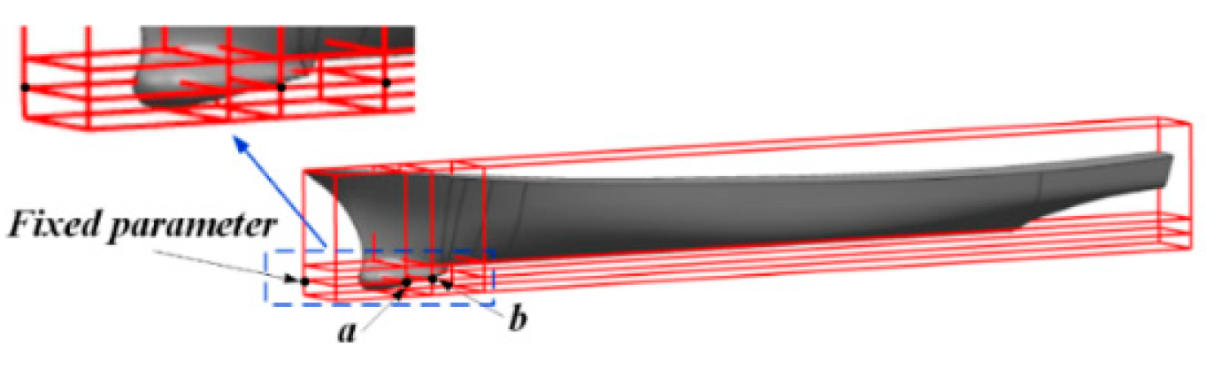
2.1. Define Optimization Problem

The Particle Swarm Optimization (PSO) method is a typical evolutionary algorithm in the global scope. This algorithm can obtain the optimal solution in the global optimization space through continuous iteration calculation. In this study, the PSO algorithm is applied to optimize the bow geometry shape of a DTMB 5512 ship model in calm water with two design variables at design speed to find the global optimal solution. In the iteration calculation, the velocity and position for different particles will be constantly updated by the following formula [25]:

$$v_i\left(j+1\right)=w\ast v_i\left(j\right)+{\mu }_1{\lambda }_1\left[a_i\left(j\right)-x_i\left(j\right)\right]+{\mu }_2{\lambda }_2\left[b_i\left(j\right)-x_i\left(j\right)\right]$$

(1)

$$x_i\left(j+1\right)=x_i\left(j\right)+v_i\left(j+1\right)$$

(2)

where w is inertia coefficient, μ₁ and μ₂ are accelerated constants, λ₁ and λ₂ are the random number from 0 to 1, x_i and v_i are the position and speed for i-th particle, respectively.

The optimization objective is to find a ship with the minimum total resistance at design speed. The total resistance R_T is obtained using the CFD method in Section 3.1. The total resistance coefficient C_T will be utilized for discussion and comparison the calculation results of the prediction and optimization, which is calculated by:

$$C_T=\frac{R_T}{0.5\rho U^{2}S}$$

(3)

where ρ is the fluid density and U is the ship speed.

According to the test method and numerical simulations, Degiuli et al. [26] pointed out that a suitable bulbous bow will decrease ship’s total resistance. Therefore, this study also modifies the sonar dome (bulbous bow) shape of the DTMB 5512 ship model to find an optimal ship hull form with minimum total resistance in calm water. Figure 1 shows the original DTMB 5512 ship model surrounded by the red control lattice. Three parameters are selected to change the ship model shape. One parameter is set as the fixed value, the other two parameters are set as the design variables in the ship hull form optimization. The position of these three parameters can be found in Figure 1. The fixed parameter is moved along the ship’s length direction, which is set as −0.20041 m. Design variables a and b are moved along the ship’s breadth direction. With the change of the bow shape, the displacement of the modified ship models will also be changed. In this study, the range of displacement for the modified ships changes from −1%Δ to 1%Δ (Δ is the displacement of the original ship model). The range of design variables a and b are set as:

0 ≤ a ≤ 0.02 m

(4)

0 ≤ b ≤ 0.02 m

(5)

2.2. Optimization Flowchart

The RANS−VOF algorithm is utilized to calculate the total resistance coefficient of different modified ship model for establishing the different surrogate models. Then, the surrogate models are applied to approximately predict the C_T of the modified ships. Finally, the PSO algorithm is applied to find the optimal ship hull form in the two−dimensional optimization space. Figure 2 shows the approximate optimization flowchart, including four steps:

• The first step is to establish the sample points. The Optimal Latin Hypercube Design (Opt LHD) algorithm is used to obtain a few samples. Then, judge whether the displacement meets the requirements. If the answer is No, change the ship’s draft to meets the constraints. If the answer is Yes, the CFD method is utilized to calculate the total resistance coefficient of modified ship models. Finally, the sample set is applied to train the surrogate model;
• Output several sets of design variables using the PSO algorithm;
• Calculate total resistance coefficient of different modified ship models using the approximate model;
• Change design variables using PSO algorithm, and repeat Steps (2)–(4) until the termination condition is satisfied. Finally, output the optimal solution with minimum total resistance coefficient.

3. Resistance Evaluation Method

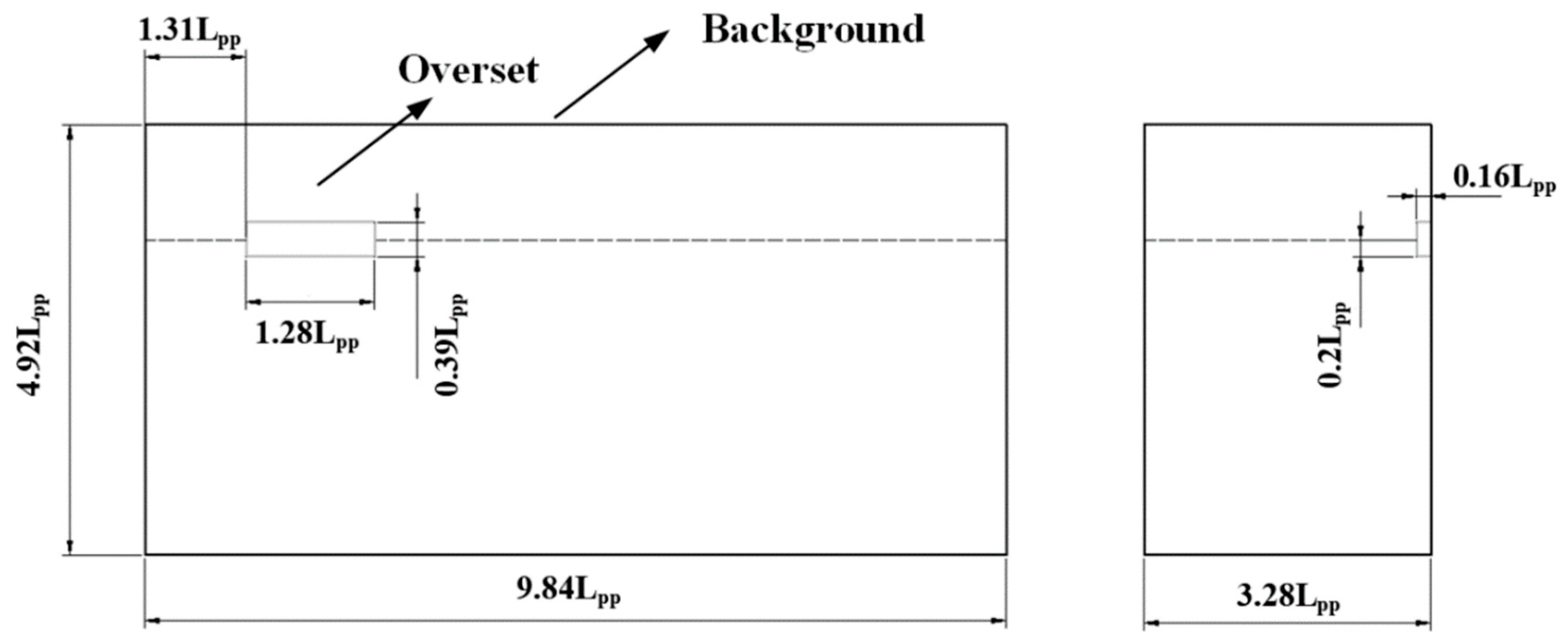
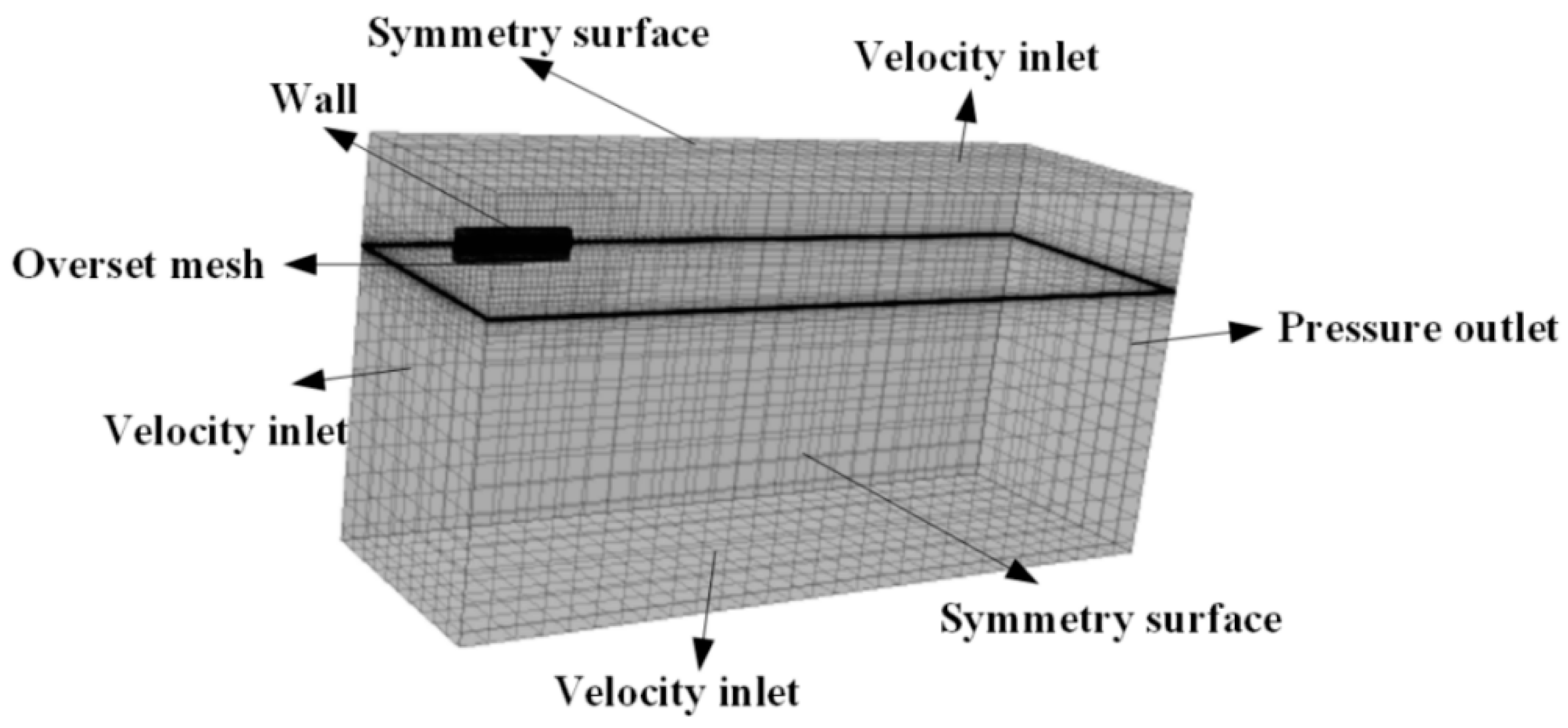
The evaluation method of the objective function is critical for the ship hull form optimization. In this section, the traditional CFD method and three surrogate models are presented.

3.1. CFD Methods

The continuity equation and the RANS equation are utilized as governing equations, as well as the realizable k−ε model throughout all the CFD simulations. The Volume of Fluid (VOF) algorithm is applied to simulate free surface between water and air phases of the CFD numerical tank. The SIMPLE algorithm is utilized to couple velocity and pressure.

The overset mesh is utilized to mesh the whole computational domain, so the background and overset blocks are established. Figure 3 shows the whole CFD numerical tank. The large cuboid is the background block, and the small cuboid is the overset block. The size of background block and overset block can be found in Figure 3.

Figure 4 reveals the boundary conditions and the mesh on the whole CFD numerical tank. The inlet, top and bottom boundaries of the background block are set as velocity inlets. The outlet boundary is set as pressure outlet. The left and the right surfaces of the background block are set as the symmetry surface. The right surface of the overset block is selected as the symmetry surface, and the ship model is set as the wall. The rest boundaries of the overset block are selected as overset mesh boundary. Mesh refining is performed on the free surface to capture the change of water surface flow field, as shown in the Figure 4. Finally, the total mesh size is approximately 1.75 million cells.

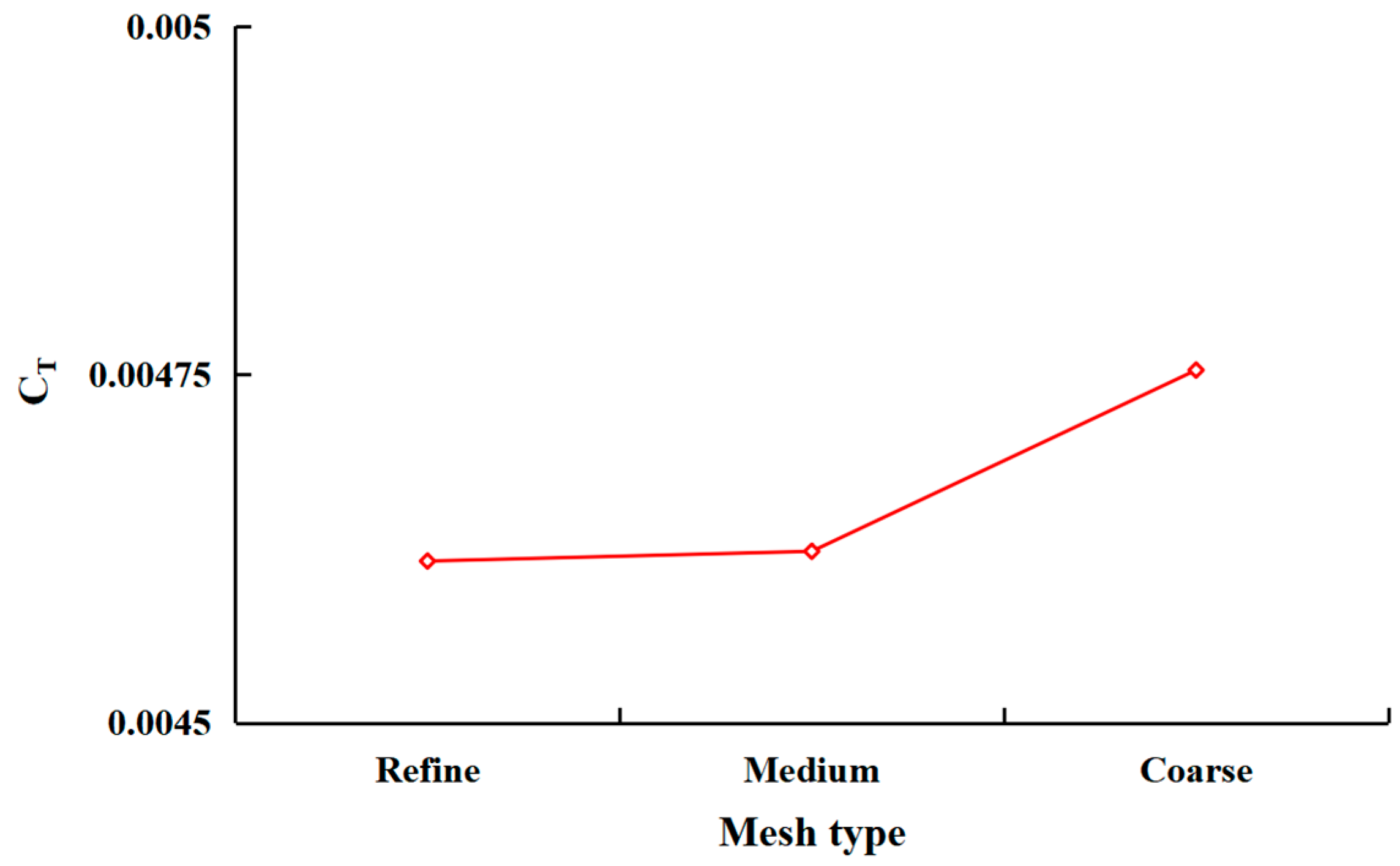
3.1.1. Validation Study for the Mesh Size

The mesh convergence study method in Tezdogan’s literature [27] is used in this study to judge the grid suitability of the current CFD model. The grids refine ratio is set as √2, which is only carried out on the overset block. Figure 5 shows the total resistance coefficients obtained using different mesh size (refine, medium and coarse mesh) by using RANS-VOF technology. The total mesh size is approximately 1.75 million and 1.26 million and 1.02 million cells for refine, medium and coarse mesh, respectively. As can be seen from Figure 5, with the decrease of the cells number, the total resistance coefficient calculated using the CFD method is increased. In addition, the total resistance coefficient has great variation from medium mesh to coarse mesh.

Table 2. The mesh convergence study in calm water.

Evaluation Parameters	Results
Convergence ratio	0.054
Extrapolated value (%)	0.46156
Approximate relative error (%)	0.15165
Extrapolation relative error (%)	0.008631
Convergence index for refine mesh	0.0108%

shows the mesh convergence study results. As can be indicated in the Table 2, the mesh tends to monotonic convergence since the convergence ratio for the present CFD model is 0.054, which is between 0 and 1. The extrapolated value and extrapolation relative error are 0.46156% and 0.008631%, respectively. Therefore, it can be conclusion that the refine mesh can be applied to simulate and calculate the total resistance of a DTMB 5512 ship model. The convergence index for refine mesh is a small uncertainty value, which is equal to 0.0108%.

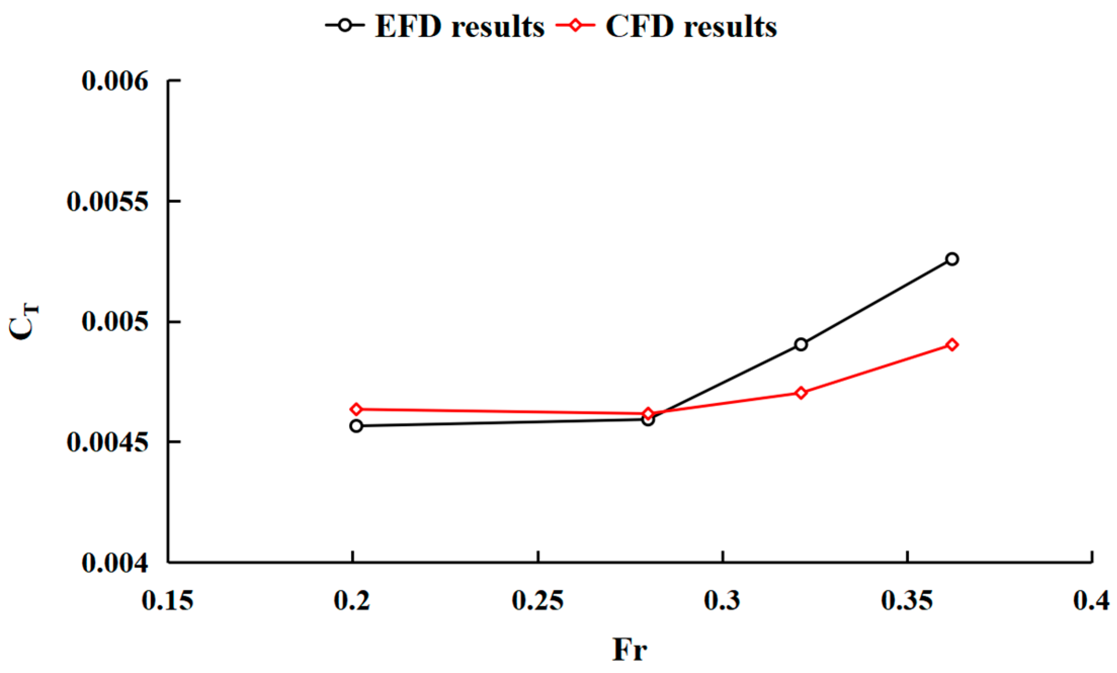
3.1.2. CFD Simulations in Calm Water

Figure 6 shows the total resistance coefficients calculated at different ship speeds between the CFD results and experimental value [28,29,30]. The average absolute error of the total resistance coefficients is approximately 3.22% at different speeds. The error is only 0.52% at design speed. As is indicated in Figure 6, the total resistance coefficients obtained using the present CFD method increased with an increase in ship speed, which agrees with the changes in experimental value. However, the total resistance error gradually increases with an increase in ship speeds. The error is approximately 4.1% at Fr = 0.3214 and 6.8% at Fr = 0.3623. A large error occurs at high speeds is possible because that the trim and sinkage motions of the ship model are not considered in the numerical simulation calculation, since high speed will increase ship motions amplitude. More importantly, this error value is within an acceptable margin. Therefore, the data lead us to the conclusion that the current CFD numerical simulation algorithm can be employed to calculate the total resistance coefficients for a DTMB 5512 ship model at design speed Fr = 0.28 in the following sections.

3.2. Surrogate Models

The surrogate model is an effective method for improving the prediction efficiency of different ship hydrodynamic performance parameters comparing to the CFD method. The following section presents three surrogate models.

3.2.1. ELMAN Surrogate Model

The ELMAN [31] surrogate model is a feedback neural network frequently, including four layers: input, hidden, context and output layers. The structure of this model can be found in Figure 7. Compared with the traditional BP model, the ELMAN surrogate model has a special context layer, which is utilized to save previous output parameter of the hidden layer. This layer can effectively improve the prediction ability of the ELMAN algorithm. The output parameter for hidden layer h( ) and output layer y( ) are [32]:

$$h\left(s\right)=f_1\left(W_1\ast x\left(s-1\right)+W_2\ast h\left(s-1\right)+\psi \right)$$

(6)

$$y\left(s\right)=f_2\left(W_3\ast h\left(s\right)+\delta \right)$$

(7)

where W₁ and W₂ and W₃ are the connection weights, x( ) is the input value in the input layer, ψ and δ are the thresholds.

3.2.2. RBF Surrogate Model

The RBF surrogate model include three layers: input, hidden and output layers. The structure of this surrogate model can be found in Figure 8. The characteristic of this surrogate model is that the hidden layer is a non−linear model, and the output layer is a linear model.

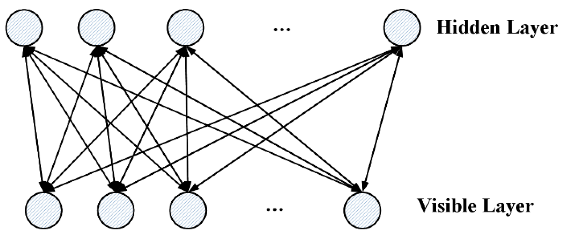
3.2.3. DBN Surrogate Model

The DBN surrogate model [35] is composed mainly of a few Restricted Boltzmann Machines (RBM) models. The structure of the RBM model can be found in Figure 9. In the DBN algorithm, the RBM model is trained one by one to obtain the corresponding parameters. The energy function for the RBM model can be obtained by [24]:

$$E(v,h|\vartheta )=-{\displaystyle \sum }_{i=1}^n{\displaystyle \sum }_{j=1}^m{v}_i{W}_{ij}{h}_j-{\displaystyle \sum }_{i=1}^n{\phi }_i{v}_i-{\displaystyle \sum }_{j=1}^m{\gamma }_j{h}_j$$

(8)

where v and h represent the parameter for visible and hidden layers, respectively. W_ij is the connection weights. φ_i and γ_j are the biases for visible and hidden layers.

The activation probability for hidden and visible layers can be calculated using [36]:

$$P(h_j=1|v,\vartheta )=\sigma \left({\gamma }_j+{\displaystyle \sum }_{i=1}^n{v}_i{W}_{ij}\right)$$

(9)

$$P(v_i=1|h,\vartheta )=\sigma \left({\phi }_i+{\displaystyle \sum }_{j=1}^m{h}_j{W}_{ij}\right)$$

(10)

where σ is the sigmoid function.

Figure 9. The structure of the RBM model [37].

Figure 9. The structure of the RBM model [37].

4. The Accuracy Evaluation for Different Surrogate Models

4.1. Data Preparation

To obtain uniform sample points, the Opt LHD method is employed to establish 200 ship hull samples in a given two−dimensional optimization space. The sample points distribution can be found in Figure 10. In addition, a subset of the sample points is presented in the

Table 3. Sample points and the corresponding C_T value.

No.	Fixed Parameter	Design Variables for Optimization		CT Obtained by CFD Method
		a	b
1	−0.20041	0.01136	0.00101	0.00453852
2	−0.20041	0.01889	0.01568	0.00451944
3	−0.20041	0.01397	0.01759	0.00451129
4	−0.20041	0.00894	0.01518	0.00450957
5	−0.20041	0.01387	0.00352	0.00457766
…	…	…	…	…
196	−0.20041	0.01528	0.01719	0.00451809
197	−0.20041	0.00704	0.01668	0.00451901
198	−0.20041	0.01266	0.00975	0.00451607
199	−0.20041	0.0197	0.01256	0.0045171
200	−0.20041	0.00281	0.01065	0.00453122

, as well as C_T for different modified ship models calculating using the RANS−VOF method.

4.2. Accuracy Evaluation for Different Surrogate Models

The 200 samples in Table 3 are used to train these 3 surrogate models (ELMAN, RBF and DBN algorithms). Another 20 new sample points, obtained using the Opt LHD algorithm, are set as the test samples to verify the calculation accuracy for the different surrogate models. The Root Mean Squared Error (RMSE) and Mean Absolute Error (MAE) and multiple correlation coefficient (R²) are selected to verify the accuracy of the prediction results for different models.

Table 4. A comparison of RMSE and MAE and R² for the total resistance coefficient prediction.

Evaluation Parameters	ELMAN Algorithm	RBF Algorithm	DBN Algorithm
RMSE	0.00115%	0.0012%	0.00093%
MAE	9.96 × 10−6	1.04 × 10−5	6.97 × 10−6
R2	0.7971	0.7508	0.9421

reveals the comparison of different evaluation parameters (RMSE, MAE and R²) for the total resistance coefficient C_T of the modified ship models. As is exhibited in the Table 4, the RMSE and MAE values calculated by using DBN algorithm are the minimum in the three surrogate models. The smaller the RMSE and MAE values of the DBN algorithm demonstrate that the calculation accuracy of the DBN model is high for the total resistance coefficient prediction. The R² value obtained using the DBN algorithm is closer to 1 than that of obtained using the ELMAN and RBF surrogate models. There is not a great deal of difference for the total resistance prediction results (RMSE, MAE and R²) using the ELMAN algorithm and RBF algorithm. The ELMAN algorithm has higher accuracy than RBF algorithm in the current prediction model. In addition, the RMSE value is from 2.03% to 2.21% for different conditions from Miao’s et al. literature [38], while the RMSE value is only 0.0011% for the DBN method. Therefore, it can be deduced that the current prediction accuracy is higher using the DBN method. Figure 11 is the error analysis results of R² by using different surrogate models. It is exhibited in the figure that the data points obtained using the DBN surrogate model are closer to the trend line than the other two surrogate models.

Figure 12 reveals the prediction results of the total resistance coefficient for different modified ship models using ELMAN, RBF and DBN algorithms. As can be indicated in Figure 12, the total resistance coefficient calculated using DBN method is much closer to CFD results than that obtained from the other two surrogate models, especially between the sample points No.1–No.7 and No.18–No.20. Therefore, it can be conclusion that the DBN algorithm are more applicable to approximately predict the total resistance coefficient of the modified DTMB 5512 ship model.

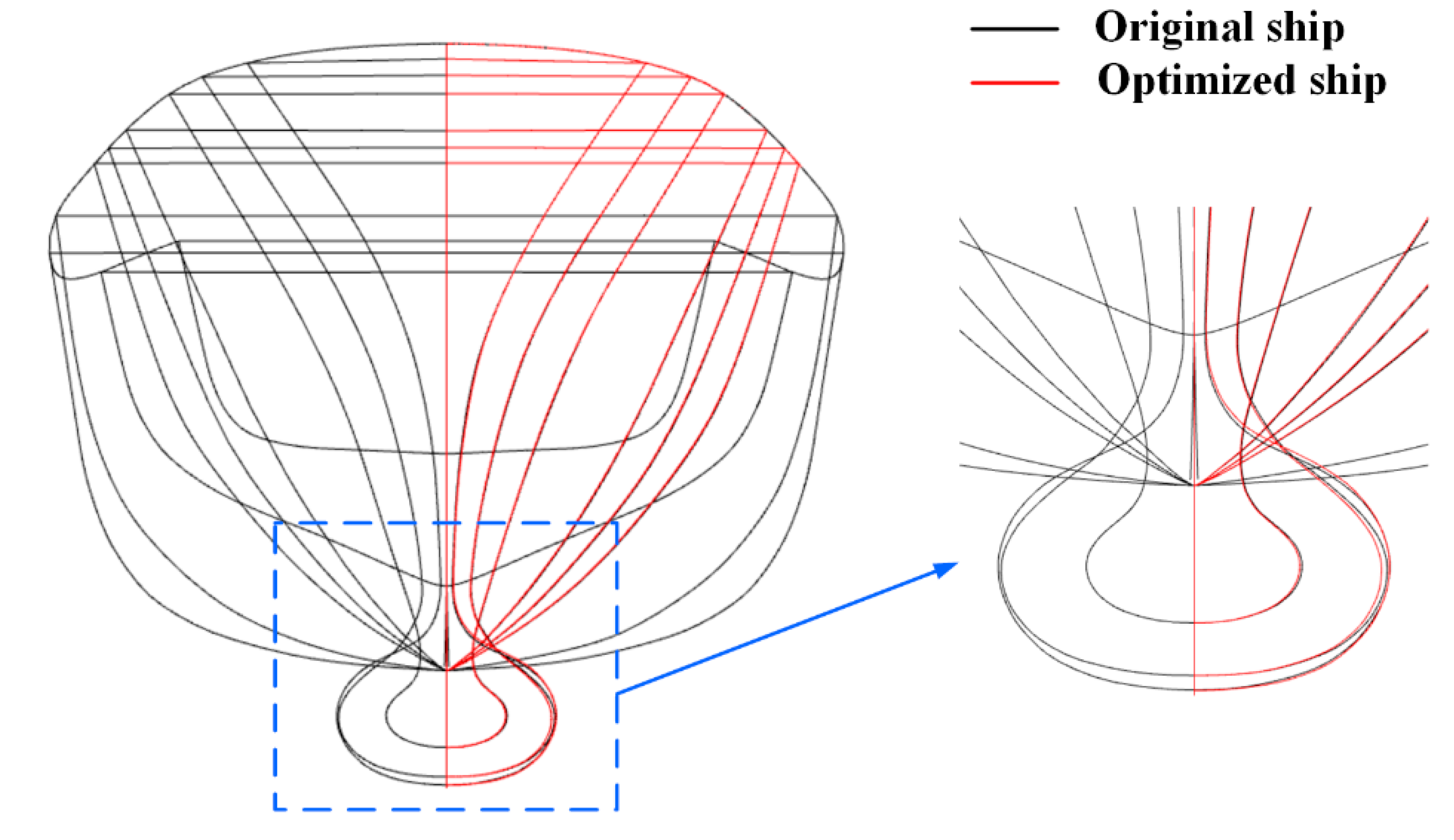
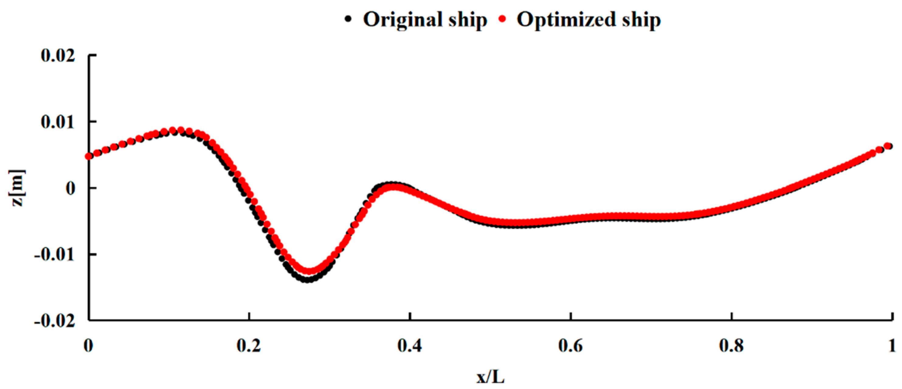
5. The Discussion for the Optimization Results

In this section, the optimization is conducted at design speed Fr = 0.28 (1.531 m/s) using the flowchart in Section 2.2. After the completion of the optimization, the optimized ship model is found with the reduction in total resistance approximately 2.37%. Figure 13 shows the ship model transversal lines for original and optimized ship models. With the change of the hull lines at bow section, the draft of the optimized ship model increases by approximately 0.01% comparing to the original ship model.

Figure 14 is a comparison of the wall shear stress distribution for original and optimized ship models. It is noticeable that the wall shear stress has a greater difference near the sonar dome between original and optimized ship models, and almost have no difference on the second half of the ship model. As is exhibited in Figure 14, the red stress region of the optimized ship model has significantly shrunken with the change of the sonar dome. In addition, the yellow stress region also reduced for the optimized ship model in comparison with the original ship model, which is good for the reduction in the total resistance of the whole ship model.

Figure 15 reveals a comparison of the wave patterns for different ship models. As is indicated in the figure, the shoulder and stern waves of the optimized ship model have significantly shrunken or disappeared compared to the original ship model due to the change of the bow shape. The result in the figure leads us to the conclusion that a suitable ship model shape will generate lower wave patterns and then will reduce the total resistance in calm water. Figure 16 is a comparison of the wave profile along different ship models at y/L = 0.0984 (y is ship’s breadth direction). As can be seen in the figure, the wave amplitude for optimal ship model is lower than that for the original ship model, especially from x/L = 0.2 to x/L = 0.4 (x is ship’s length direction).

Figure 17 is a comparison of total resistance coefficient obtained using for original and optimized ship models at different ship speeds. It is worth mentioning from the figure that the C_T of the optimized ship model has been reduced at all speeds. The maximum resistance reduction of the optimized ship model is occurred at low ship speed. The resistance decreases by approximately 5.83% and 5.18% at Fr = 0.201 and Fr = 0.241, respectively, while with the increase of the ship speed, the resistance reduction effect is weakened. The resistance decreases by approximately 2.37% and 2.47% and 2.02% at the other three ship speeds sequentially. Compared with the original ship model, the average total resistance coefficient C_T of the optimized ship model decreases by 3.57% for five ship speeds. Although the single objective optimization method is used in this study to optimize the DTMB 5512 ship model, the total resistance reduction effect of the optimized ship model is satisfactory not only at design speed but also at the other four ship speeds.

6. Conclusions and Recommendation for Future Work

This paper proposed a new ship hull form optimization method using DBN technology for reducing the total resistance in calm water. First of all, the RANS and VOF methods were utilized to calculate the total resistance of the original DTMB 5512 ship model. The calculation results indicate that the current CFD method can be employed to calculate the total resistance of a DTMB 5512 ship model in calm water, with the average error of 3.22% at four different ship speeds. Then, the CFD method and Opt LHD were integrated to obtain the sample ship models for the sake of training the surrogate models. To verify the calculation accuracy of the DBN algorithm, the common surrogate models (ELMAN and RBF) were also applied in this study to predict the total resistance for different modified DTMB 5512 ship models. The results show that the total resistance prediction results obtained using the DBN method are superior to that obtained using the ELMAN and RBF methods. Following this, an approximate ship hull form optimization is carried out using two design variables. Finally, the optimized ship model has been found. The total resistance of this optimized ship model reduced by approximately 2.37% compared to the original ship model with a draft variation of approximately 0.01% at design speed. The average total resistance of the optimized ship model exhibits a 3.57% decrease over five ship speed setpoints presented in this study.

In this paper, the total resistance of the DTMB 5512 ship calculated using the CFD method has a big error at high speed. Further studies will calculate the total resistance of this ship considering ship motions in calm water to shrink error at high speeds. In addition, only the total resistance of the DTMB 5512 ship model was predicted and compared using different surrogate models. Further studies will consider different surrogate models to forecast other hydrodynamic performance parameters (heave and pitch motions, promotion efficiency of the propeller and so on) of a DTMB 5512 ship model. Moreover, the applicability of the deep belief network technology to predict different hydrodynamic parameters will be discussed in the future.

References

1. Zha, L.; Zhu, R.; Hong, L.; Huang, S. Hull form optimization for reduced calm-water resistance and improved vertical motion performance in irregular head waves. Ocean Eng. 2021, 233, 109208. [Google Scholar] [CrossRef]
2. Qiang, Z.; Feng, B.; Liu, Z.; Chang, H.; Wei, X. Optimization method for hierarchical space reduction method and its application in hull form optimization. Ocean. Eng. 2022, 262, 109208. [Google Scholar] [CrossRef]
3. Nazemian, A.; Ghadimi, P. CFD-based optimization of a displacement trimaran hull for improving its calm water and wavy condition resistance. Appl. Ocean Res. 2021, 113, 102729. [Google Scholar] [CrossRef]
4. Zhao, C.; Wang, W.; Jia, P.; Xie, Y. Marine Design and Research Institute of China optimisation of hull form of ocean-going trawler. Brodogradnja 2021, 72, 33–46. [Google Scholar] [CrossRef]
5. Ding, D.; Yao, R.; Luo, N.; Zhou, Y.; Wang, X.; Yu, L. Lines optimization for a medium cruise ship based on rapidity. Ship Eng. 2022, 44, 1–7. [Google Scholar]
6. Hamed, A. Multi-objective optimization method of trimaran hull form for resistance reduction and propeller intake flow improvement. Ocean Eng. 2021, 244, 110352. [Google Scholar] [CrossRef]
7. Huang, F.; Yang, C. Hull form optimization of a cargo ship for reduced drag. J. Hydrodyn. 2016, 28, 173–183. [Google Scholar] [CrossRef]
8. Solak, H.P. Multi-dimensional surrogate based aft form optimization of ships using high fidelity solvers. Brodogradnja 2020, 71, 85–100. [Google Scholar] [CrossRef]
9. Liu, X.; Zhao, W.; Wan, D. Hull form optimization based on calm-water wave drag with or without generating bulbous bow. Appl. Ocean Res. 2021, 116, 102861. [Google Scholar] [CrossRef]
10. Zhang, W.; Zhou, J.; Yu, B.; Yu, Y. Research on model building for bulbous bow resistance optimization based on BPNN. J. Dalian Univ. Technol. 2021, 61, 160–171. [Google Scholar]
11. Tian, X.; Sun, X.; Liu, G.; Xie, Y.; Chen, Y.; Wang, H. Multi-objective optimization of the hull form for the semi-submersible medical platform. Ocean Eng. 2021, 230, 109038. [Google Scholar] [CrossRef]
12. Shang, Y.; Zhao, L. Optimization of profile and side-hull spacing of wind turbine operation and maintenance catamaran based on radial basis function. China Offshore Platf. 2022, 37, 70–75. [Google Scholar]
13. Liu, X.; Zhao, W.; Wan, D. Multi-fidelity Co-Kriging surrogate model for ship hull form optimization. Ocean Eng. 2021, 243, 110239. [Google Scholar] [CrossRef]
14. Feng, Y.; Chen, Z.; Dai, Y.; Cui, L.; Zhang, Z.; Wang, P. Multi-objective optimization of a bow thruster based on URANS numerical simulations. Ocean Eng. 2022, 247, 110784. [Google Scholar] [CrossRef]
15. Ouyang, X.; Chang, H.; Liu, Z.; Feng, B.; Zhan, C.; Cheng, X. Application of adaptive sampling method in hull form optimization. J. Shanghai Jiaotong Univ. 2022, 56, 937–943. [Google Scholar]
16. Wan, Y.; Hou, Y.; Xiong, Y.; Dong, Z.; Zhang, Y.; Gong, C. Interval optimization design of a submersible surface ship form considering the uncertainty of surrogate model. Ocean Eng. 2022, 263, 112262. [Google Scholar] [CrossRef]
17. de Baar, J.; Roberts, S.; Dwight, R.; Mallol, B. Uncertainty quantification for a sailing yacht hull, using multi-fidelity kriging. Comput. Fluids 2015, 123, 185–201. [Google Scholar] [CrossRef] [Green Version]
18. Hou, Y.; Huang, S.; Liang, X. Ship hull optimization based on PSO training FRBF neural network. J. Harbin Eng. Univ. 2017, 38, 175–180. [Google Scholar]
19. Luo, W.; Guo, X.; Dai, J.; Rao, T. Hull optimization of an underwater vehicle based on dynamic surrogate model. Ocean Eng. 2021, 230, 109050. [Google Scholar] [CrossRef]
20. Wu, G.; Ma, W.; Liu, C.; Wang, S. IOT and cloud computing based parallel implementation of optimized RBF neural network for loader automatic shift control. Comput. Commun. 2020, 158, 95–103. [Google Scholar] [CrossRef]
21. Chu, H.; Wei, J.; Wu, W. Streamflow prediction using LASSO-FCM-DBN approach based on hydro-meteorological condition classification. J. Hydrol. 2019, 580, 124253. [Google Scholar] [CrossRef]
22. Li, Y.; Peng, T.; Hua, L.; Ji, C.; Ma, H.; Nazir, M.S.; Zhang, C. Research and application of an evolutionary deep learning model based on improved grey wolf optimization algorithm and DBN-ELM for AQI prediction. Sustain. Cities Soc. 2022, 87, 104209. [Google Scholar] [CrossRef]
23. Xi, Y.; Zhao, J.; Lin, D.; Yu, L.; Chen, G.; Zhang, J.; Li, B.; Li, F.; Jiang, Y. Transformer evaluation and life prediction method based on DBN and health index. Electron. Device 2022, 45, 878–882. [Google Scholar]
24. Wang, M.; Wang, H.; Wang, J. Wear volume prediction of brake shoes used in heavy freight wagon based on DBN. Comput. Simul. 2022, 39, 134–139. [Google Scholar]
25. Huang, S.; Jiang, L.; Li, Z.; Yang, G.; Song, F. Corona loss prediction of UHV AC transmission line based on DBN neural network optimized by PSO. Electr. Power 2022, 55, 95–102. [Google Scholar]
26. Degiuli, N.; Farkas, A.; Martić, I.; Zeman, I.; Ruggiero, V.; Vasiljević, V.; Vienna Model Basin Ltd. Numerical and experimental assessment of the total resistance of a yacht. Brodogradnja 2021, 72, 61–80. [Google Scholar] [CrossRef]
27. Tezdogan, T.; Incecik, A.; Turan, O. Full-scale unsteady RANS simulations of vertical ship motions in shallow water. Ocean Eng. 2016, 123, 131–145. [Google Scholar] [CrossRef] [Green Version]
28. Gui, L.; Longo, J.; Stern, F. Biases of PIV measurement of turbulent flow and the masked correlation-based interrogation algorithm. Exp. Fluids 2001, 30, 27–35. [Google Scholar] [CrossRef]
29. Gui, L.; Longo, J.; Stern, F. Towing tank PIV measurement system, data and uncertainty assessment for DTMB Model 5512. Exp. Fluids 2001, 31, 336–346. [Google Scholar] [CrossRef]
30. Longo, J.; Stern, F. Uncertainty Assessment for Towing Tank Tests With Example for Surface Combatant DTMB Model 5415. J. Ship Res. 2005, 49, 55–68. [Google Scholar] [CrossRef]
31. Elman, J.L. Finding structure in time. Cogn. Sci. 1990, 14, 179–211. [Google Scholar] [CrossRef]
32. Zhao, D. Prediction model for the height of water flowing fractured zones based on ELMAN neuran network. Shanxi Coal 2022, 42, 8–14. [Google Scholar]
33. Shi, X.H. Some Theoretical Studies of ELMAN Neural Networks and Evolutionary Algorithms and Their Applications; Jilin University Press: Changchun, China, 2006. [Google Scholar]
34. Feng, M.F.; Lu, J.C. Study on short time traffic flow prediction based on RBF neural network optimized by PSO. Comput. Simul. 2010, 27, 323–326. [Google Scholar]
35. Hinton, G.E.; Osindero, S.; Teh, Y.-W. A Fast Learning Algorithm for Deep Belief Nets. Neural Comput. 2006, 18, 1527–1554. [Google Scholar] [CrossRef]
36. Wang, F. Retrieval and Recommendation System of Resources Based on Deep Belief Networks; Beijing University of Posts and Telecommunications Press: Beijing, China, 2015. [Google Scholar]
37. Bengio, Y. Learning deep architectures for AI. Found. Trends® Mach. Learn. 2009, 2, 1–127. [Google Scholar] [CrossRef]
38. Miao, A.; Zhao, M.; Wan, D. CFD-based multi-objective optimization of S60 Catamaran considering demihull shape and separation. Appl. Ocean. Res. 2020, 97, 102071. [Google Scholar] [CrossRef]
Figure 1. Design variables distribution for changing the original ship model.
Jmse 10 01735 g001
Figure 2. Flow chart of the ship hull form optimization loop.
Jmse 10 01735 g002
Figure 3. The dimensions of the CFD numerical tank for two regions.
Jmse 10 01735 g003
Figure 4. The boundary conditions and the mesh on the whole CFD numerical tank.
Jmse 10 01735 g004
Figure 5. The total resistance coefficients CT obtained using different mesh types.
Jmse 10 01735 g005
Figure 6. The total resistance coefficient CT for CFD results and experimental value.
Jmse 10 01735 g006
Figure 7. The structure of the ELMAN surrogate model [33].
Jmse 10 01735 g007
Figure 8. The structure of the RBF surrogate model [34].
Jmse 10 01735 g008
Figure 10. Sample space distribution for two−dimensional space obtained using the Opt LHD algorithm.
Jmse 10 01735 g010
Figure 11. Error analysis for R2 using different surrogate models. (a) Error analysis for R2 using the ELMAN surrogate model. (b) Error analysis for R2 using the RBF surrogate model. (c) Error analysis for R2 using the DBN surrogate model.
Jmse 10 01735 g011
Figure 12. Comparison of the total resistance coefficient CT for different methods. (a) Comparison of the CT for CFD and ELMAN results. (b) Comparison of the CT for CFD and RBF results. (c) Comparison of the CT for CFD and DBN results.
Jmse 10 01735 g012
Figure 13. The body plan of the original and optimized ship models.
Jmse 10 01735 g013
Figure 14. The wall shear stress distribution for different ships.
Jmse 10 01735 g014
Figure 15. The wave patterns for different ship models.
Jmse 10 01735 g015
Figure 16. The profile of the wave profile along different ship models at y/L = 0.0984.
Jmse 10 01735 g016
Figure 17. Total resistance coefficient changes with ship speeds for different ship models.
Jmse 10 01735 g017