Numerical Simulation of Wave Overtopping of an Ecologically Honeycomb-Type Revetment with Rigid Vegetation

Abstract

Traditional concrete revetments can destroy the ecological environment and the water landscape. An increasing number of ecological revetment structures have been applied in coastal, lake, and river regulation projects. It has been found that honeycomb-type revetments display a better performance in the attenuation of wave overtopping when compared to experimental data collected using the Eurotop and Muttray’s formula; recording a 40% decrease in the wave run-up in comparison to the latter. To further investigate the wave run-up and overtopping of the ecologically vegetated honeycomb-type revetment, based on OpenFOAM, an open source computational fluid dynamics software, a three-dimensional numerical wave tank was established. The Discrete Particle Method (DPM) was used to simulate gravel movement, and the flexible plant move boundary model was developed to simulate vegetation. The results of wave run-up calculated by the numerical model and those obtained by the experiments were in good agreement, with errors less than 20%. The modeled results of wave overtopping were within the same order of magnitude as those from the experiments; however, critical limitations were noticed due to effects of plant generalization and grid restrictions imposed by DPM methods. The results showed that wave overtopping increased with increasing wave period and wave height. However, with an increase in the wave overtopping, the influence of the wave period on wave overtopping decreased. The increase in vegetation density effectively reduced wave overtopping. Furthermore, an empirical formula for wave overtopping, considering the effects of vegetation density, was proposed.

1. Introduction

In river and coastal areas, revetments play important roles in defending against floods and waves. Recently, ecological revetments have attracted increased attention. As a new type of ecological revetment, the ecologically vegetated honeycomb-type revetment [1], which combines vegetation with geotextile honeycomb structures, has both good protective properties and the function of restoring the ecological environment. It is significant to the hydrodynamic characteristics and stability of the structure to investigate the wave run-up and overtopping of the vegetated honeycomb-type revetment.

Wave overtopping of revetments has always been of great interest, and many studies have been carried out through theoretical analysis [2,3,4], experiments [5,6,7,8], and numerical models [9,10,11,12]. With the development of computer technology, numerical simulation has become one of the major measures by which to study wave overtopping. The numerical simulation method can choose various numerical models, including nonlinear shallow water (NLSW) equation model, Boussinesq equation model, Navier-Stokes equation model, smoothed particle hydrodynamics (SPH) model, and nonhydrostatic model.

The NLSW equation simplifies the wave-breaking processes and applies them to shallow water, with slower changes in slope and less vertical velocity. Based on the total variation diminishing (TVD) schemes to solve NLSW equation s and the SWASH model, an improved numerical model was separately adopted to simulate wave overtopping on an impermeable mound breakwater [13,14]. The results of the numerical model are compared with the physical model test results, and demonstrate that the model is robust and reliable for the prediction of wave overtopping on sea dikes.

The Boussinesq equation model can describe fluid particle motion, reflects the nonlinear characteristics of wave motion, and has a wider applicability, which can simulate the wave transformation in moderate water depth. McCabe et al. established a semi-implicit shallow water Boussinesq equation model, in which the wave breaking and overtopping of random waves on curved and steep sloping seawalls were considered [15].

Recently, the SPH model, based on the Langrange method and capable of tracking the large deformations of the free surface with good accuracy, has been used to simulate wave overtopping processes. Shao [16] presented an incompressible smoothed particle hydrodynamics (SPH) model to investigate wave overtopping of coastal structures. The computations were validated against experimental and numerical data, and a good agreement was observed.

A nonhydrostatic model can accurately accommodate large gradients and discontinuities in flows with fewer vertical mesh layers. Based on the nonhydrostatic wave model SWASH, Zhang et al. [17] used the equivalent drag method to simulate wave overtopping on a mound breakwater covered by an accropode, and established an empirical formula that considered the equivalent bottom friction coefficient of the accropode blocks.

Most models designed to investigate flow within a porous media are based on Navier-Stokes (NS) equations. When using the NS equations, two different Lagrangian and Eulerian approaches have been followed in the numerical modeling of wave propagation and its interaction with structures [18]. Losada et al. [19,20] established the COBRAS (Cornell breaking waves and structures) model based on the VARANS equations, and used VOF to investigate the functionality of rubble mound breakwaters, with special attention focused on wave overtopping processes. By introducing the Darcy-Forchheimer equation into N–S equation, Li et al. [21] established a numerical model considering the interaction between wave and porous media based on VARANS equations and OpenFOAM, to simulate the wave overtopping over permeable breakwater covered by armor blocks with irregular wave, by accurately describing the geometric shape of the accropodes in the numerical wave tank. Higuera [22,23] found a new solver, IHFOAM, by introducing the VARANS equations into Open-FOAM, then studied the overtopping of oblique random waves over a 3D porous high-mound breakwater at prototype scale.

The abovementioned studies mainly focused on the interaction between traditional revetment and wave, and did not consider the influence of vegetation.

The bottom friction factor is generally used to reflect the plants’ effect on waves in numerical simulations of vegetation dissipation characteristics. According to experimental data, an empirical model applied to the rough bottom friction factor was proposed [24,25]. With the improvements in computer performance, vegetation is considered a solid boundary; generalizing vegetation into certain geometric shapes and directly solving the flow fields with plant boundaries. Based on OpenFOAM, an open source program, a solver, IHFoam, was developed that considers plants as rigid cylinders to solve the flow field and wave forces [26,27]. However, the model has not yet been applied in ecological revetments.

The progress of wave run-up and overtopping on revetments with plant protection is a coupling process of waves, vegetation, gravel, and a honeycomb structure. DPM was first used in the simulation of 3D bed-load sediment motion by Schemeeckle [28], Drake [29], and Mcewan [30], without considering bidirectional coupling. However, the unidirectional function was not enough to describe the motion under water-sediment interaction, so now the coupling of computational fluid dynamics (CFD) and the Discrete Particle Model (DPM) is widely used in the simulation of water-sediment movements [31,32,33,34,35,36]. To reasonably simulate wave run-up and overtopping over honeycomb ecological revetments with rigid vegetation, this study was based on OpenFOAM, an open source computational fluid dynamics software, and combines bidirectional coupling calculations of CFD and DPM. In this study, irregularly shaped gavels were equivalent to spherical particles, vegetation was generalized into rigid cylinders, and a three-dimensional numerical wave tank was established that considers particle movement. Simulations of overtopping over honeycomb revetments with vegetation was carried out, the influence of wave period, wave height, and vegetation density on overtopping were discussed, and an empirical formula of overtopping under the influence of plants was proposed.

2. Numerical Model

A two-phase flow solver with the Discrete Particle Method (DPM) was combined to simulate the fluid-solid interaction, based on OpenFOAM. A three-dimensional numerical wave flume considering particle motion was established, in which plant and honeycomb structures were treated as fixed wall boundaries, and gravel in honeycomb cells was simulated by the DPM.

2.1. Numerical Wave Tank

The continuity equation and momentum equation are:

$$\nabla \cdot U=0$$

(1)

$$\frac{\partial \rho U}{\partial t}+\nabla \cdot (\rho UU)=\nabla \cdot \left(\mu \nabla U\right)+\nabla \mu \cdot {\left(\nabla U\right)}^{\mathrm{T}}+C\kappa \nabla \alpha -\nabla p_{rgh}-gh\nabla \rho$$

(2)

where U is the velocity of the fluid; $\rho$ is the fluid density; $\mu$ is the dynamic viscosity coefficient of the fluid; C is the surface tension coefficient, which is usually taken as 0.07; $\kappa$ is the curvature of the interface; and $\alpha$ is the volume fraction. $p_{rgh}$ is the correction pressure of the fluid;

$$p_{rgh}=p-\rho gh$$

(3)

where $p$ is the total pressure, $g$ is the gravity acceleration, and $h$ is the water depth.

The Reynolds time-averaged RANS equation is used as the basic governing equation of the fluid mathematical model.

The volume of fluid (VOF) method, proposed by Hirt et al., is used to capture free surfaces of numerical wave tank. It is a free surface tracking method commonly used in multiphase flow numerical simulations. The VOF method does not directly track the movement of fluid particles; the basic principle is to determine the position of the free surface by solving a phase fraction based on the ratio of fluid volume to grid cell volume. The value of the phase fraction (α) ranges from 0 to 1:0 means that the unit is completely air, 1 means that the unit is completely liquid, and 0 to 1 means that the unit is a mixture of air and liquid.

In the specific solution process of two-phase flow, gas and liquid are considered as a mixed fluid, and weighted value by phase fraction. The basic physical properties of the mixed fluid can be expressed as follows:

$$\rho =\alpha {\rho }_l+(1-\alpha ){\rho }_a$$

(4)

$$\mu =\alpha {\mu }_l+(1-\alpha ){\mu }_a$$

(5)

where $\rho$ is the density of the mixed fluid; ${\rho }_l$ is the density of the liquid; ${\rho }_a$ is the density of air; $\mu$ is the dynamic viscosity coefficient of the mixed fluid; ${\mu }_l$ is the dynamic viscosity coefficient of the liquid; and ${\mu }_a$ is the dynamic viscosity coefficient of air.

In VOF, the phase fraction needs to satisfy the phase Equation (6), which is a hyperbolic differential equation, and it is difficult to directly solve the boundary conditions on the free surface. In the calculation, by adding an artificial compression term to the left side of Equation (7), the value of this term is 0 in the pure gas phase and the pure liquid phase (i.e., $\alpha =0$ and $\alpha =1$), which is only valid in the gas–liquid mixed phase (i.e., $0\prec \alpha \prec 1$).

$$\frac{\partial \alpha }{\partial t}+\alpha \frac{\partial u_i}{\partial x_i}=0$$

(6)

$$\frac{\partial \alpha }{\partial t}+\alpha \frac{\partial u_i}{\partial x_i}+\alpha \left(1-\alpha \right)\frac{\partial u_i}{\partial x_i}=0$$

(7)

The OpenFOAM solver adopted in this study uses the MULES method to solve the phase fraction to determine the position of the free surface.

2.2. CFD-DPM Coupling Model

A CFD-DPM model was adopted, which consists of the computation of fluid, particles, and fluid-particles coupling. The calculation of fluid was locally based on the volume-averaged Navier–Stokes (VARANS) equation, the particles motion was calculated by solving the rigid translation and rotation equation, and the collision of particles was described based on the soft sphere model proposed by Cundall [37], as based on the DPM. Additionally, a forcing equation was required to close the two-phase equation, since the influence of particles on fluid were considered as point sources without calculating analytically the force on the particles surface by meshing.

2.2.1. The Computation of Fluid Phase and Particle Phase

The VARANS equations were used as the governing equation of fluid, which are shown as:

$$\frac{\partial {\alpha }_f}{\partial t}+\nabla \cdot \left({\alpha }_f{u}_f\right)=0$$

(8)

$$\frac{\partial \left({\alpha }_f{u}_f\right)}{\partial t}+\nabla \cdot \left({\alpha }_f{u}_f{u}_f\right)=-\frac{1}{{\rho }_f}\nabla p+\frac{1}{{\rho }_f}\nabla \cdot \left({\alpha }_f\mathbf{\tau }\right)+{\alpha }_f{f}_{ext}+\frac{1}{{\rho }_f}{\alpha }_f{f}_{pf}$$

(9)

where ${\alpha }_f$ is the volume fraction of fluid, $u_f$ and ${\rho }_f$ are the velocity and density of fluid, respectively; $\tau =\mu \left(\nabla u_f+\nabla u_f{}^T\right)$ is the stress tensors in fluid microelements; $f_{ext}$ is the external forces on fluid, including gravity; and $f_{pf}$ is the mean inherent volume value of fluid-sand force in the control volume units.

The computation of the particles’ translation and rotation is based on Newton’s second law, shown as:

$$m_a\frac{d{U}_a}{dt}=F_{contact,a}+F_{ext,a}$$

(10)

$$I_a\frac{d{\Omega }_a}{dt}=T_{contact,a}+T_{ext,a}$$

(11)

where $U_a$ and ${\Omega }_a$ respectively represent the translational speed and rotational speed of particle a; $F_{contact,a}$ represents the impact force between particle a and surrounding particles; $F_{ext,a}$ represents the external force acting on particle a, such as the force of fluid on the particle, gravity, and lubricating force; $T_{contact,a}$ represents the collision moment between particle a and surrounding particles; and $T_{ext,a}$ represents the external movement acting on the particle a, such as the movement generated by the water flow on the particle.

The impact force generated during the collision of two contacting particles is calculated by the linear spring and buffer model, proposed by Cundall et al. [37]. The impact force on particle a is the join force when it comes into contact with other surrounding particles b, which includes normal force $F_{ab,n}$ and shear force $F_{ab,t}$:

$$F_{contact,a}={\displaystyle \sum _{\forall b\in contactlist}\left(F_{ab,n}+F_{ab,t}\right)}$$

(12)

The normal force $F_{ab,n}$ is computed by using the Hertzian contact theory [38], expressed as:

$$F_{ab,n}=-k_n{\delta }_{ab,n}^{3/2}-{\eta }_n{U}_{ab,n}$$

(13)

where $U_{ab,n}$ is the normal relative velocity between particle a and particle b; $k_n$ is normal spring stiffness coefficient; ${\eta }_n$ is normal viscous dissipation coefficient; ${\mathbf{\delta }}_{ab,n}$ is the normal component of the overlapping displacement between two particles.

The shear force $F_{ab,t}$ is computed considering two different particle contact modes: rolling friction and sliding friction. Elastic collision is used to compute $F_{ab,t}$, as it is static friction between particle a and particle b ($\left|F_{ab,t}\right|\le {\mu }_s\left|F_{ab,n}\right|$); but, as sliding friction between particle a and particle b ($\left|F_{ab,t}\right|>{\mu }_s\left|F_{ab,n}\right|$), the classical Coulomb friction law is used to describe $F_{ab,t}$:

$$F_{ab,t}=\left\{\begin{array}{l}-k_t{\delta }_{ab,t}-{\eta }_t{U}_{ab,t},\left|F_{ab,t}\right|\le {\mu }_s\left|F_{ab,n}\right|\\ -{\mu }_s\left|F_{ab,n}\right|t_{ab},\left|F_{ab,t}\right|>{\mu }_s\left|F_{ab,n}\right|\end{array}\right.$$

(14)

$k_t$ is the shear spring stiffness coefficient, ${\mu }_s$ is sliding friction coefficient, ${\eta }_t$ is viscous dissipation coefficient.

2.2.2. The Coupling of Fluid and Particle

In a DPM model, the force of the particle on fluid $f_{pf}$ and that of the fluid on particle $F_{fp,i}$ are the relationship between force and reactive force within a unit volume (intrinsic average) in the momentum equation:

$$\frac{1}{V_{cell}}{\displaystyle {\int }_{S_{pf}}\left(-p{n}_{pf}+\tau \cdot n_{pf}\right)dS}={\alpha }_f{f}_{pf}=-\frac{{\displaystyle {\sum }_{i=1}^{N_p}{F}_{fp,i}}}{V_{cell}}$$

(15)

where $V_{cell}$ is the volume of computing cell, $S_{pf}$ is the fluid-solid surface area in computing units, ${\alpha }_f$ is fluid volume friction (or porosity), $F_{fp,i}$ is force of fluid on particle $i$ in computing units, $N_p$ is total number of particles in $V_{cell}$.

As an important feature of the vegetated honeycomb-type revetment, the gravel can be simulated by using a DPM model just considering the one-way influence of fluid on particle. However, a DPM model is not enough to describe the particle movement under the fluid-particles interaction. In a CFD-DPM model, with two-way coupling computation, particle stability analysis can be carried out and the scour situation of the surface on vegetated honeycomb-type revetment can be obtained. This is because the gravel movement under waves and the impact of gravel particles can be simulated using CFD-DPM, due to the simplification of gravel to spherical particles. In addition, the particle gradation can be considered in CFD-DPM.

2.3. DPM-VOF Coupling Model

To simulate the wave run-up on the revetment, VOF is added to the CFD-DPM model. Then, an air-fluid-particle interaction model (DPMInterFoam) is established, with the following governing equation:

$$\frac{\partial \left({\alpha }_f{\alpha }_1\right)}{\partial t}+\nabla \cdot \left({\alpha }_f{\alpha }_1{u}_f\right)+\nabla \cdot \left({\alpha }_f{\alpha }_1\left(1-{\alpha }_1\right)u_r\right)=0$$

(16)

where $u_f$ is the velocity of fluid; $u_r$ is the relative velocity, known as the compression velocity, and specifically refers to the velocity difference of two grids closest to the interface; ${\alpha }_f$ is the volume fraction of fluid and air, namely, ${\alpha }_f=\left(V_1+V_2\right)/V_c$; $V_1$ and $V_2$ are the volumes of fluid and air, respectively; $V_c$ is the total volume of grids; and ${\alpha }_1$ is the ratio of fluid volume to total volume of fluid and air. The discrete equations can be expressed as:

$$\frac{\partial \left({\alpha }_1{\alpha }_f\right)}{\partial t}+{{\displaystyle \sum _F\left[\left({\alpha }_f{\alpha }_1\right)u_f\right]}}_F\cdot S_F+{{\displaystyle \sum _F\left[{\alpha }_f{\alpha }_1\left(1-{\alpha }_1\right)u_r\right]}}_F\cdot S_F=0$$

(17)

where $S_F$ represents the area vector of surface $F$, the direction points out of the cell, and F represents the number of faces.

3. Validations

3.1. Brief Introduction of Physical Model Experiment

To validate the accuracy of the numerical model, a physical model test was carried out in the Port and Coastal Engineering Laboratory of Tianjin University. The geometric scale and time scale were chosen as 1:10 and 1:3.6, respectively, according to gravity similarity criterion. The size of the wave tank was 35 m × 1 m × 1 m. In the experiments, the height of the revetment section model was 0.7 m, the slope was 1:3.5, and the length was 2.1 m. The core of the revetment section model was filled with bricks, which were covered by sand. The sand was covered by a layer of geotextile, and the geotextile was covered by a honeycomb of gravel. The section is shown in Figure 1 and Figure 2.

In the study, there were six sets of experiments. The height of the first three sets was 0.1 m, the depth was 0.46 m, and the periods were 1.26 s, 1.58 s, and 1.9 s, respectively. The depth of the last three sets was 0.63 m, which was the experimental set to have overtopping. The above sets were experimental scenarios 1 to 6, which are shown in

Table 1. Experimental conditions.

	Wave Height	Wave Period	Depth	Wave Overtopping
Case 1	Model 0.1 m Prototype 1 m	Model 1.26 s Prototype 4.536 s	Model 0.46 m Protytope 4.6 m	No
Case 2	Model 0.1 m Prototype 1 m	Model 1.58 s Prototype 5.688 s	Model 0.46 m Prototype 4.6 m	No
Case 3	Model 0.1 m Prototype 1 m	Model1.9 s Prototype 6.840 s	Model 0.46 m Prototype 4.6 m	No
Case 4	Model 0.1 m Prototype 1 m	Model 1.26 s Prototype 4.536 s	Model 0.63 m Prototype 6.3 m	Yes
Case 5	Model 0.1 m Prototype 1 m	Model 1.58 s Prototype 5.688 s	Model 0.63 m Prototype 6.3 m	Yes
Case 6	Model 0.1 m Prototype 1 m	Model1.9 s Prototype 6.840 s	Model 0.63 m Prototype 6.3 m	Yes

.

The wave run-up was image-processed from the video captured by a Canon EOS60D camera. The overtopping wave was first collected by the water tank, and then pumped into a 2-L measuring cylinder to measure the volume, taken by the self-priming pump. The water surface process curves and wave parameters were monitored and collected by eight wave height sensors. In the experiment, 200 waves were collected at a frequency of 40 times per second, and the statistical characteristics, such as average wave height and duration, were recorded after the waveform collected by the last sensor was stable. A DS-30 multi-point wave height meter was used in the experiment, and a DJ800 multi-function monitoring system was used for data analysis and statistics. There were errors in the wave height sensor, and probably in the difference of wave height values between that made by the wave maker and that at the toe of revetment. Therefore, calibrations of the wave height sensor and wave maker were made before conducting the experiment to obtain the correct wave height.

3.2. Establishment of Vegetated Honeycomb-Type Revetment Model

In the numerical wave tank, the irregularly shaped gravels were equivalent to spherical particles. In the experiments, the quality of the gravels ranged from 0.003 to 0.006 kilograms, and the density was 2650 kg/m³; therefore, the diameters of the spherical particles ranged from 0.0129 m to 0.0163 m. The honeycomb grilles were treated as solid boundaries due to their impermeable characteristics.

In the DPM method, the size of the minimum mesh needed to be Δx = Δy = Δz = 0.02 m, which was larger than the particle diameter, namely, 0.0129~0.0163 m. After the honeycomb grid was divided, the particles naturally settled. After the particles fell into the honeycomb, the position of the particles in the natural accumulation state were obtained, as shown in Figure 3.

Suaeda was used as the plant in the honeycomb experiment with vegetation. The branch and trunk of the plant were relatively rigid and did deform greatly under the wave conditions used in the experiment. Therefore, the plant was considered to have approximate rigidity. Due to the limitation of grid accuracy, each Suaeda plant could not be accurately depicted in the numerical flume. Referring to previous studies conducted on the problem of wave attenuation due to plants, the plant was equivalent to a simple rigid cylinder [25,26], and the Suaeda plant was determined equivalent to a square column to participate in the calculation of the flow field due to the grid accuracy, which was not high enough to describe the shape of the cylinder.

A single Suaeda plant group was composed of approximately 10–20 branches with different heights, and the base cross-sectional area of each plant was approximately 0.000004 m². In the maximum vegetation density scenario, the density was approximately 1000 plants/m², for a total of approximately 2300 plants. There was a total of 144 honeycomb cancellus, with an average of 18 branches per cancellus. The cross-sectional area of the branches was approximately 0.0092 m². The projected area of plant stems and leaves was more complicated, and it was impossible to accurately calculate the projected area. Considering the influence of branches and leaves, the plants in a cancellus were generalized into a square column, as shown in Figure 3. A square column was chosen with side lengths of 0.018 m, 0.019 m, 0.020 m, 0.021 m, and 0.022 m to establish a model corresponding to the experiment. By comparing the simulation results with the experimental results, the sensitivity analysis was performed on the side length of the square column. The analysis showed that when the side length of the square column was 0.02 m, the simulation results were in the highest agreement with the experimental results.

3.3. Model Verification

Figure 4 shows the process of wave run-up and wave overtopping simulated by the numerical model.

Table 2. Comparison between the run-up height of the experiments and that of the numerical simulation (Unit: m).

	Honeycomb Revetment without Plants			Honeycomb Revetment with Plants
	Experiment	Numerical Simulation	Error	Experiment	Numerical Simulation	Error
Case 1	0.081	0.070	13%	0.079	0.065	18%
Case 2	0.100	0.098	2%	0.087	0.082	5%
Case 3	0.116	0.116	0%	0.093	0.099	6%

shows the climbing height and comparison of the two revetment experiments, and numerical simulation calculations. When the wave height was constant, in both the experiment and the numerical simulation, the climbing height showed an increased trend with increased wave period, and the error between the two decreased with the increased climbing height. The climbing height of the revetment with plants was smaller than that of a gravel revetment.

At the designed high water level of 0.63 m, some sets of waves had overtopping, and the average per width wave overtopping was used to measure the wave overtopping. The specific calculation method used was: Q = V/(B t), where Q is per width average wave overtopping, V is total volume of the wave overtopping, t is time, and B is the width of the top of the revetment.

The comparison between the average per-width average wave overtopping, measured in the experiment, and the average per-width average wave overtopping, calculated in the numerical model, is shown in

Table 3. Comparison between the per-width averaged wave overtopping of the experiments and that of the numerical simulation (Unit: m³/(m·s)).

	Honeycomb Revetment without Plants			Honeycomb Revetment with Plants
	Experiment	Numerical Simulation	Error	Experiment	Numerical Simulation	Error
Case 4	3.37 × 10−4	2.37 × 10−4	29%	2.6 × 10−6	9.3 × 10−6	257%
Case 5	7.88 × 10−4	8.53 × 10−4	8%	1.39 × 10−5	2.18 × 10−5	57%
Case 6	1.45 × 10−3	1.448 × 10−3	0.1%	3.07 × 10−5	4.3 × 10−5	40%

. From the experimental data, it can be concluded that, when compared with the experimental group of gravels, the wave overtopping drastically decreased on the revetment with plants. In the three sets of experiments with plants, due to the influence of plants, the wave overtopping, which was caused by the splashing of water droplets, was very small on the experimental section with a width of 1 m in a one wave period. Due to the generalization of plants, which could not fully reflect the influence of real plants and had limited accuracy due to the limitations of the grid, the results obtained by the numerical model had a significant error in terms of percentage, especially when the wave overtopping was small. However, the values were not much different and were within an order of magnitude, so the numerical model still had a certain degree of accuracy.

In addition, according to the experiment,

Table 4. Comparison between the run-up height of the vegetated honeycomb-type revetment and that calculated using Muttray’s formula. (Unit: m).

$\mathbf{Mean} \mathbf{Incident} \mathbf{Wave} \mathbf{Height} \mathit{H}$ (m)	$\mathbf{Wave} \mathbf{Period} \mathit{T}$ (s)	$\mathbf{Depth} \mathit{d}$ (m)	Plant Density/Height	Experimental Result	Calculation Result of Muttray	Ratio of Difference to Calculation Result
0.06	1.58	0.46	750 plants/m2	5	8.1	38.27%
0.08	1.58	0.46	1000 plants/m2	5.5	10.6	48.11%
0.1	1.58	0.46	0.10 m	7.7	13	40.77%
0.1	1.58	0.46	0.20 m	7.3	13	43.85%

and

Table 5. Comparison between the per-width averaged wave overtopping of the vegetated honeycomb-type revetment and that calculated from Eurotop formula. (Unit: m³/(m·s)).

$\mathbf{Mean} \mathbf{Incident} \mathbf{Wave} \mathbf{Height} \mathit{H}$ (m)	$\mathbf{Wave} \mathbf{Period} \mathit{T}$ (s)	$\mathbf{Depth} \mathit{d}$ (m)	Plant Density/Height	Experimental Result	Calculation Result of Eurotop	Ratio of Difference to Calculation Result
0.1	1.9	0.63	750 plants/m2	2.59 × 10−4	4.42 × 10−4	41.40%
0.1	1.9	0.63	1000 plants/m2	7.41 × 10−5	3.87 × 10−4	80.85%
0.1	1.9	0.63	0.10 m	3.07 × 10−5	3.87 × 10−4	92.07%
0.1	1.9	0.63	0.20 m	1.37 × 10−5	3.87 × 10−4	96.46%

show that, due to the honeycomb-type revetment, the wave overtopping decreased compared with the Eurotop formula, and the wave run-up decreased by around 40% compared with Muttray’s formula. It was found that, due to the honeycomb-type revetment, the wave overtopping decreased compared with the Eurotop formula, and the wave runup decreased by around 40% compared with Muttray formula.

4. Effect of Honeycomb Revetment with a Rigid Plant on Wave Overtopping

4.1. Case Setting

The revetment slope was 1:3.5; the revetment top height was 0.9 m; the revetment width was 1 m; the water depth was 0.8 m; and the height of the honeycomb structure was 0.1 m. The gravel weighed 3 to 6 g, with an irregular geometric shape, and it was replaced by spherical particles with a diameter of 0.0129 m to 0.0163 m. The density of the gravel was 0.6. The total number of honeycombs was approximately 50,000. A pot of Suaeda plants was replaced by a square pillar with a side length of 0.02 m, and the plant heights were uniformly set as 0.2 m. The plant density was artificially set as low density and high density. Low density was considered to be 1 pot of Suaeda per honeycomb cell, which corresponded to a plant density of 500 plants/m² in the experiment, and the degree of stem and leaf cover was 33.25%. High density was considered to be 2 pots of Suaeda per honeycomb cell, and corresponded to a plant density of 1000 plants/m² in the experiment, and the degree of stem and leaf cover was 66.5%. These are shown in Figure 5.

Due to the limitations of the DPM, the grid size must be larger than the particles, and the grid along the water depth direction was taken to be 0.02 m, so the minimum wave height was set to 0.1 m. The grid had difficulty accurately describing the water surface, and wave overtopping did not occur when the wave height was less than 0.1 m. In the calculation case, the water depth was 0.8 m. In the numerical wave flume, if the ratio of wave height to water depth was greater than 1/3, the wave broke during the propagation process, which affected the calculation of the wave overtopping. Therefore, the maximum wave height was set to 0.28 m. The minimum wave period of the wave period was 1.2 s, and the maximum wave period was set to 3.3 s. Therefore, in the calculation of numerical simulation, there were seven types of wave heights, at 0.1 m, 0.12 m, 0.14 m, 0.16 m, 0.18 m, 0.22 m, and 0.28 m; the wave periods were 1.2 s, 1.5 s, 1.9 s, 2.3 s, 2.7. s, 3.0 s, and 3.3 s; plants were considered either low density and high density; and a total of 56 working conditions were calculated. The calculation conditions for low and high density were the same, as shown in

Table 6. Low (high) density group conditions.

	T (s)	H (m)		T (s)	H (m)		T (s)	H (m)
Case 1	1.2	0.1	Case 11	1.9	0.16	Case 21	2.7	0.28
Case 2	1.2	0.12	Case 12	1.9	0.22	Case 22	3.0	0.1
Case 3	1.2	0.14	Case 13	1.9	0.28	Case 23	3.0	0.16
Case 4	1.2	0.16	Case 14	2.3	0.1	Case 24	3.0	0.22
Case 5	1.5	0.1	Case 15	2.3	0.16	Case 25	3.0	0.28
Case 6	1.5	0.12	Case 16	2.3	0.22	Case 26	2.7	0.28
Case 7	1.5	0.14	Case 17	2.3	0.28	Case 27	3.3	0.28
Case 8	1.5	0.16	Case 18	2.7	0.1	Case 28	1.5	0.22
Case 9	1.5	0.18	Case 19	2.7	0.16
Case 10	1.9	0.1	Case 20	2.7	0.22

.

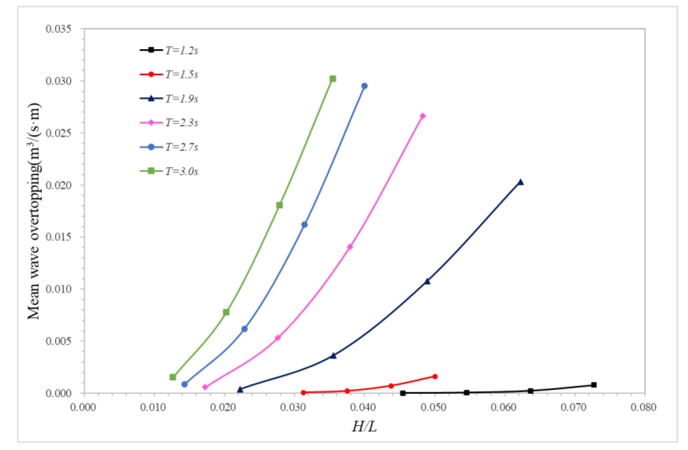
4.2. Effect of Wave Period on the Wave Overtopping

4.2.1. Low Vegetation Density

In the low-density group, wave heights are $H$ = 0.1 m and 0.16 m; the wave periods are $T$ = 1.2 s, 1.5 s, 1.9 s, 2.3 s, 2.7 s, and 3.0 s; and the corresponding wavelength is $L$ = 2.2 m, 3.2 m, 4.5 m, 5.8 m, 7 m, and 7.9 m. As shown in Figure 6, the wave overtopping is generally small when the wave height is $H$ = 0.1 m, and there is essentially no wave overtopping under short wave periods. As the wave period increases, the wave overtopping exponentially increases. When $H$ = 0.16 m, the wave overtopping still increases as the wave period increases, but the growth trend is basically linear, and it can be observed that, as the period increases and the wave overtopping gradually increases, the growth rate of the wave overtopping has a slowing trend.

In the low-density group, the wave height is $H$ = 0.22 m; the wave periods are $T$ = 1.5 s, 1.9 s, 2.3 s, 2.7 s, and 3.0 s; and the corresponding wavelengths are $L$ = 3.2 m, 4.5 m, 5.8 m, 7 m, and 7.9 m. When $T$ = 1.2 s, the wave has broken during the propagation process, and the target wave height cannot be reached at the foot of the revetment. As shown in Figure 6, when $H$ = 0.22 m, the wave overtopping in each group is already relatively large, and although the wave overtopping still increases with the wave period, the growth rate significantly slows down when the period is relatively large.

In the low vegetation density group, the wave height is $H$ = 0.28 m; wave periods are $T$ = 1.9 s, 2.3 s, 2.7 s, 3.0 s, and 3.3 s; and the corresponding wavelengths are $L$ = 3.2 m, 4.5 m, 5.8 m, 7 m, 7.9 m, and 8.8 m. When $T$ = 1.5 s, the wave has broken during propagation, and the target wave height cannot be reached at the foot of the revetment. To ensure that there were enough data points to observe the trend, the case of $T$ = 3.3 s was added. As shown in Figure 6, under the wave height condition, the increasing speed of wave overtopping with increasing wave period significantly slows down. Particularly, when wave overtopping is greater than 0.03 m³/ (s·m), the growth rate significantly slows down.

4.2.2. High Vegetation Density

The high vegetation density corresponds to a vegetation density of 1000 plants/m² in the experiment. Compared with the low vegetation density group, because of the distribution of vegetation, the turbulence in the water was promoted, the water energy was dissipated, and the resistance received during the propagation increased, then the wave was significantly weakened. Therefore, due to the wave dissipation effect of vegetation, not only does the wave overtopping significantly decrease, but the changing trends of the wave overtopping on the revetment and wave period also differ under the same wave height in the high vegetation density group.

When the wave height is $H$ = 0.1 m in the high-density group, the wave periods are $T$ = 1.2 s, 1.5 s, 1.9 s, 2.3 s, 2.7 s, and 3.0 s; and the corresponding wavelengths are $L$ = 2.2 m, 3.2 m, 4.5 m, 5.8 m, 7 m, and 7.9 m. As shown in Figure 7, when the wave height is $H$ = 0.1 m, the wave overtopping still exponentially increases as the wave period increases.

When the wave height is $H$ = 0.16 m in the high-density group, the wave periods are $T$ = 1.2 s, 1.5 s, 1.9 s, 2.3 s, 2.7 s, and 3.0 s; and when the wave height is $H$ = 0.22 m, the wave periods are $T$ = 1.5 s, 1.9 s, 2.3 s, 2.7 s, and 3.0 s. In the low-density group, when $H$ = 0.16 m, the wave overtopping linearly increases with increasing wave overtopping, but when $H$ = 0.22 m, the growth rate of the wave overtopping slows down. However, as shown in Figure 7, in the high-density group, when $H$ = 0.16 m and $H$ = 0.22 m, the wave overtopping still shows a linear increase with an increasing wave period.

In the high-density group, when the wave height is $H$ = 0.28 m, the wave periods are $T$ = 1.9 s, 2.3 s, 2.7 s, 3.0 s, and 3.3 s; and the corresponding wavelengths are $L$ = 2.2 m, 3.2 m, 4.5 m, 5.8 m, 7 m, 7.9 m, and 8.8 m. As shown in Figure 7, after the initial linear growth of the wave overtopping, the growth rate significantly slows down after the wave overtopping exceeds 0.026 m³/(s·m), but wave overtopping does not increase when the wave period increase has not occurred yet.

4.3. Effect of Wave Height on Wave Overtopping

Cases with the same period and different wave heights were selected for analysis. For example, the cases with wave period $T$ = 1.2 s and wave heights $H$ = 0.1 m, 0.12 m, 0.14 m, and 0.16 m, were selected to draw the curve of the wave overtopping changing with the wave height. A total of six curves for the low-density group with $T$ = 1.2 s, 1.5 s, 1.9 s, 2.3 s, 2.7 s, and 3.0 s are plotted in Figure 8.

Figure 8 shows that the wave overtopping exponentially increases as the wave height increases until the wave breaks, with no trend of slowing down. The wave period affects the speed of exponential growth. In the stage when the wave height is small, the growth rate of short-period waves is much lower than that of long-period waves. With the wave height increasing, the growth rate of short-period waves and long-period waves gradually increase.

For the high-density group, the wave overtopping was significantly reduced, but compared with the low-density group, the trend of the wave overtopping with wave height did not change in the high-density group; it still exponentially increased, and the effect of the wave period on the growth rate was also consistent.

4.4. Effect of Vegetation Density on Wave Overtopping

Cases with the same period and wave heights and different vegetation density were selected for analysis. A total of four curves for the decrease percentage of wave overtopping with different vegetation densities are plotted in Figure 9.

Figure 9 shows that, with the vegetation density increasing from 500 plants/m² to 1000 plants/m², wave overtopping over the vegetated honeycomb-type revetment presents a downward trend. The overtopping volume decreases by about 10~70% with the decrease in vegetation density.

4.5. Empirical Formula Fitting of the Wave Overtopping Considering the Effect of Rigid Plants

Overtopping predictions by generic formulas bear significant uncertainties. Based on the simulation results above, a formula was proposed which can directly use a vegetated sloped structure. For traditional sloped structures, based on numerous physical model experiments and field observation results, many scholars both domestically and abroad have proposed empirical formulas [38,39,40,41] in which the influence of vegetations were not directly considered. However, considering wave overtopping on sloped revetments with plants presents a problem with wave overtopping on sloped buildings in nature, the selection of an empirical formula form can refer to the existing function model. A function model, similar to the Eurotop formula, was adopted and nondimensionalization of the wave overtopping, Q*, was carried out, as shown in Equation (18). From the above, when the wave height was constant, there was a certain relationship between wave overtopping and wavelength. Therefore, the relationship between the dimensionless coefficient, Q*, and the dimensionless coefficient, H/L, was investigated, as shown in Figure 10, and the two dimensionless coefficients displayed a good correlation. In a certain wave period, there was a evident relationship between overtopping and wave height. In this case, the top height, R_c, of the revetment was used to nondimensionalize the wave height, so the relationship between the dimensionless coefficient, Q*, and the dimensionless coefficient, H/R_c, was investigated, as shown in Figure 11, and the two dimensionless coefficients also had a good correlation.

$$Q^{*}=\frac{Q}{\sqrt{g{H}_s^3}}$$

(18)

The fitted empirical formula is Equation (19), and the specific form can be determined as Equation (20) by referring to the formula of Eurotop, where C is a parameter related to plant density. The value of this parameter varies with different densities.

$$\mathrm{f}\left(\frac{Q}{g{H}_s^3},\frac{H}{L},\frac{H}{R_c}\right)=0$$

(19)

$$\frac{Q}{\sqrt{g{H}_s^3}}=A\frac{\sqrt{\tan \alpha }}{{\left(H/L\right)}^D}\exp \left[-B{\left(\frac{R_c{\left(H/L\right)}^D}{C\tan \alpha H}\right)}^E\right]$$

(20)

The formula was fitted using Origin. The data of the low (high) density group calculated by numerical simulation were fitted. The fitting result of numerical simulation data is Equation (21):

$$\frac{Q}{\sqrt{g{H}_{}^3}}=0.07\frac{\sqrt{\tan \alpha }}{{\left(H/L\right)}^{0.3}}\exp \left[-0.5{\left(\frac{R_c{\left(H/L\right)}^{0.3}}{0.458\tan \alpha H}\right)}^{2.3}\right]$$

(21)

The calculated value $Q^{\prime }=\frac{Q}{\sqrt{g{H}_{}^3}}$, obtained by the empirical Equation (21), are compared with the numerical simulation result $Q^{*}$, as shown in Figure 12. The oblique line in the figure is an ideal line at 45°. The results show that the calculated value of the wave overtopping obtained by the empirical formula has a good correlation with the numerical simulation result, and the square of the correlation coefficients is R₂ = 0.980, respectively.

5. Conclusions

Based on OpenFOAM, an open source computational fluid dynamics software, this study established a three-dimensional numerical wave tank, considered the movement of particles and rigid plants, and carried out numerical simulation research on wave run-up and wave overtopping of honeycomb revetments with vegetation. The main conclusions were as follows:

(1)

Based on OpenFOAM, the two-phase flow solver was combined with the Discrete Particle Model solver to establish the air-water-particle three-phase interaction model while considering the influence of plants. Several physical model experimental groups of honeycomb ecological revetment with vegetation were selected, and the correctness of the model was verified by comparing the wave run-up height, water level in sensors, and wave overtopping in the physical model test with the numerical simulation results.

(2)

The honeycomb-type ecological revetment model with the protection of plants was used to simulate the wave overtopping process of regular waves on honeycomb revetments, with plants under various wave conditions and different vegetation densities. Through analysis of the numerical simulation results, it was found that with increased wave height and wave period, the overtopping also gradually increased; but, with increased wave overtopping, the influence of the wave period on the overtopping gradually weakened. The increase in vegetation density could only effectively reduce wave overtopping, but does not change the trend of wave overtopping in terms of wave height and wave period.

(3)

Referring to the Eurotop formula, the relationship between Q* and the dimensionless coefficients H/R_c and H/L was established, and the empirical formula for overtopping the honeycomb-type ecological revetment model with plants was fitted according to the numerical modelling results. Parameter C in the formula was related to plant density.

References

1. Phillips, B.M. Design of Streambank Stabilization with Geogrid Reinforced Earth Systems. In Proceedings of the Joint Conference on Water Resource Engineering and Water Resources Planning and Management 2000, Minneapolis, MN, USA, July 30–2 August 2000; pp. 1–10. [Google Scholar]
2. Yuan, S.; Tang, H.; Li, L.; Pan, Y.; Amini, F. Combined wave and surge overtopping erosion failure model of HPTRM levees: Accounting for grass-mat strength. Ocean Eng. 2015, 109, 256–269. [Google Scholar] [CrossRef] [Green Version]
3. Kreyenschulte, M.; Schürenkamp, D.; Bratz, B.; Schüttrumpf, H.; Goseberg, N. Wave Run-Up on Mortar-Grouted Riprap Revetments. Water 2020, 12, 3396. [Google Scholar] [CrossRef]
4. Vieira, F.; Taveira-Pinto, F.; Rosa-Santos, P. Novel time-efficient approach to calibrate VARANS-VOF models for simulation of wave interaction with porous structures using Artificial Neural Networks. Ocean Eng. 2021, 235, 109375. [Google Scholar] [CrossRef]
5. Bakker, P.; Reedijk, B.; Manaois, J.R.; van de Koppel, M.; Muttray, M. Causes for Increased Wave Overtopping on Rubble Mound Breakwaters and Revetments. In Coasts, Marine Structures and Breakwaters 2017: Realising the Potential; Thomas Telford Limited: London, UK, 2018; pp. 1205–1215. [Google Scholar]
6. Schoonees, T.; Kerpen, N.B.; Schlurmann, T. Full-scale experimental study on wave overtopping at stepped revetments. Coast. Eng. 2021, 167, 103887. [Google Scholar] [CrossRef]
7. Capel, A. Wave run-up and overtopping reduction by block revetments with enhanced roughness. Coast. Eng. 2015, 104, 76–92. [Google Scholar] [CrossRef]
8. Warmink, J.J.; van Bergeijk, V.M.; Chen, W.; Van Gent, M.R.; Hulscher, S.J.M. Modelling wave overtopping for grass covers and transitions in dike revetments. Coast. Eng. Proc. 2018, 36, 53. [Google Scholar] [CrossRef] [Green Version]
9. Alcérreca-Huerta, J.C.; Oumeraci, H. Wave-induced pressures in porous bonded revetments. Part I: Pressures on the revetment. Coast. Eng. 2016, 110, 87–101. [Google Scholar] [CrossRef]
10. Cao, D.; Yuan, J.; Chen, H. Towards modelling wave-induced forces on an armour layer unit of rubble mound coastal revetments. Ocean Eng. 2021, 239, 109811. [Google Scholar] [CrossRef]
11. Chen, W.; Warmink, J.J.; Van Gent, M.R.A.; Hulscher, S.J.M.H. Numerical modelling of wave overtopping at dikes using OpenFOAM®. Coast. Eng. 2021, 166, 103890. [Google Scholar] [CrossRef]
12. Yao, Y.; Chen, X.; Xu, C.; Jia, M.; Jiang, C. Numerical modelling of wave transformation and runup over rough fringing reefs using VARANS equations. Appl. Ocean Res. 2022, 118, 102952. [Google Scholar] [CrossRef]
13. Tuan, T.Q.; Oumeraci, H. A numerical model of wave overtopping on seadikes. Coast. Eng. 2010, 57, 757–772. [Google Scholar] [CrossRef]
14. Li, T.; Troch, P.; Rouck, J.D. Wave overtopping over a sea dike. J. Comput. Phys. 2004, 198, 686–726. [Google Scholar] [CrossRef]
15. Mccabe, M.; Stansby, P.K.; Apsley, D.D. Random wave runup and overtopping a steep sea wall: Shallow-water and Boussinesq modelling with generalised breaking and wall impact algorithms validated against laboratory and field measurements. Coast. Eng. 2013, 74, 33–49. [Google Scholar] [CrossRef]
16. Shao, S.; Ji, C.; Graham, D.I.; Reeve, D.E.; James, P.W.; Chadwick, A.J. Simulation of wave overtopping by an incompressible SPH model. Coast. Eng. 2006, 53, 723–725. [Google Scholar] [CrossRef]
17. Zhang, N.; Zhang, Q.; Wang, K.H.; Zou, G.; Li, Y. Numerical Simulation of Wave Overtopping on Breakwater with an Armor Layer of Accropode Using SWASH Model. Water 2020, 12, 386. [Google Scholar] [CrossRef] [Green Version]
18. Losada, I.J.; Lara, J.L.; Jesus, M.D. Modeling the Interaction of Water Waves with Porous Coastal Structures. J. Waterw. Port Coast. Ocean Eng. ASCE 2016, 6, 142. [Google Scholar] [CrossRef]
19. Losada, I.J.; Lara, J.L.; Guanche, R.; Gonzalez-Ondina, J.M. Numerical analysis of wave overtopping of rubble mound breakwaters. Coast. Eng. 2008, 55, 47–62. [Google Scholar] [CrossRef]
20. Lara, J.L.; Garcia, N.; Losada, I.J. RANS modelling applied to random wave interaction with submerged permeable structures. Coast. Eng. 2006, 53, 395–417. [Google Scholar] [CrossRef]
21. Li, J.Y.; Zhang, Q.H.; Lu, Y.J. Numerical Simulation of Random Wave Overtopping of Rubble Mound Breakwater with Armor Units. China Ocean Eng. 2021, 35, 176–185. [Google Scholar] [CrossRef]
22. Higuera, P.; Lara, J.L.; Losada, I.J. Realistic wave generation and active wave absorption for Navier–Stokes models: Application to OpenFOAM. Coast. Eng. 2013, 71, 102–118. [Google Scholar] [CrossRef]
23. Higuera, P.; Lara, J.L.; Losada, I.J. Three-Dimensional Interaction of Waves and Porous Coastal Structures using OpenFOAM. Part II: Applications. Coast. Eng. 2014, 83, 259–270. [Google Scholar] [CrossRef]
24. Augustin, L.N.; Irish, J.L.; Lynett, P. Laboratory and numerical studies of wave damping by emergent and near-emergent wetland vegetation. Coast. Eng. 2009, 56, 332–340. [Google Scholar] [CrossRef]
25. Manca, E.; Cáceres, I.; Alsina, J.M.; Stratigaki, V.; Townend, I. Wave energy and wave-induced flow reduction by full-scale model Posidonia oceanica seagra. Cont. Shelf Res. 2012, 50–51, 100–116. [Google Scholar] [CrossRef]
26. Maza, M.; Lara, J.L.; Losada, I.J. Tsunami wave interaction with mangrove forests: A 3-D numerical approach. Coast. Eng. 2015, 98, 33–54. [Google Scholar] [CrossRef]
27. Maza, M.; Lara, J.L.; Losada, I.J. Solitary wave attenuation by vegetation patches. Adv. Water Resour. 2016, 98, 159–172. [Google Scholar] [CrossRef]
28. Schmeeckle, M.W. The Mechanics of Bedload Sediment Transport; Bell & Howell Information Company: Arbor, MI, USA, 1998. [Google Scholar]
29. Drake, T.G.; Calantoni, J. Discrete particle model for sheet flow sediment transport in the nearshore. J. Geophys. Res. 2001, 106, 859–868. [Google Scholar] [CrossRef]
30. McEwan, I.K.; Heald, J. Discrete Particle Modeling of Entrainment from Flat Uniformly Sized Sediment Beds. J. Hydraul. Eng. 2001, 127, 588–597. [Google Scholar] [CrossRef] [Green Version]
31. Xu, S.L.; Sun, R.; Cai, Y.Q.; Sun, H.l. Study of sedimentation of non-cohesive particles via CFD–DEM simulations. Granul. Matter 2017, 20, 4. [Google Scholar] [CrossRef] [Green Version]
32. Sun, R.; Xiao, H. CFD–DEM simulations of current-induced dune formation and morphological evolution. Adv. Water Resour. 2016, 92, 228–239. [Google Scholar] [CrossRef] [Green Version]
33. Finn, J.R.; Li, M.; Apte, S.V. Particle based modelling and simulation of natural sand dynamics in the wave bottom boundary layer. J. Fluid Mech. 2016, 796, 340–385. [Google Scholar] [CrossRef]
34. Schmeeckle, M.W. Numerical simulation of turbulence and sediment transport of medium sand. J. Geophys. Res. Earth Surf. 2014, 119, 1240–1262. [Google Scholar] [CrossRef]
35. Kafui, K.D.; Thornton, C.; Adams, M.J. Discrete particle-continuum fluid modelling of gas–solid fluidised beds. Chem. Eng. Sci. 2002, 57, 2395–2410. [Google Scholar] [CrossRef]
36. Arolla, S.K.; Desjardins, O. Transport modeling of sedimenting particles in a turbulent pipe flow using Euler-Lagrange large eddy simulation. Int. J. Multiph. Flow 2015, 75, 1–11. [Google Scholar] [CrossRef] [Green Version]
37. Cundall, P.A.; Strack, O. A discrete numerical model for granular assemblies. Géotechnique 2008, 30, 331–336. [Google Scholar] [CrossRef]
38. Crowe, C.T.; Schwarzkopf, J.D.; Sommerfeld, M.; Tsuji, Y. Multiphase Flows with Droplets and Particles; CRC Press: Boca Raton, FL, USA, 2011. [Google Scholar]
39. Goda, Y. Random Seas and Design of Maritime Structures; World Scientific Publishing Co. Pte. Ltd.: Singapore, 1924. [Google Scholar]
40. Code of Hydrology for Harbor and Waterway. 2015, JTS 145-2015. Available online: https://www.nssi.org.cn/nssi/english/88067670.html (accessed on 14 October 2022).
41. Van der Meer, J.W.; Allsop, N.W.H.; Bruce, T.; Rouck, J.D.; Zanuttigh, B. EurOtop: Manual on Wave Overtopping of Sea Defences and Related Sturctures: An Overtopping Manual Largely Based on European Research, but for Worlwide Application. Available online: www.overtopping-manual.com (accessed on 1 June 2022).
Figure 1. Experimental section with Suaeda.
Jmse 10 01615 g001
Figure 2. Schematic diagram of the experimental section.
Jmse 10 01615 g002
Figure 3. Schematic diagram of the model adding generalized plants. (a) Honeycomb-type revetment without gravel and vegetation; (b) Honeycomb-type revetment with rigid vegetation; (c) Honeycomb-type revetment without rigid vegetation.
Jmse 10 01615 g003
Figure 4. The process of wave run-up and wave overtopping simulated by the numerical model.
Jmse 10 01615 g004
Figure 5. Schematic diagram with two vegetation densities. (a) High vegetation density; (b) Low vegetation density.
Jmse 10 01615 g005
Figure 6. Wave overtopping with a certain wave height and different g T 2 / a .
Jmse 10 01615 g006
Figure 7. Wave overtopping with a certain wave height and different g T 2 / a .
Jmse 10 01615 g007
Figure 8. Wave overtopping with a certain wave period and different wave steepness.
Jmse 10 01615 g008
Figure 9. Decrease of wave overtopping with different vegetation densities.
Jmse 10 01615 g009
Figure 10. Relationship between dimensionless parameter Q* and H/L.
Jmse 10 01615 g010
Figure 11. Relationship between dimensionless parameter H/Rc and Q*.
Jmse 10 01615 g011
Figure 12. Comparison between the calculated value of the empirical formula and the numerical simulation result.
Jmse 10 01615 g012