Numerical Modeling of the Impact of Sea Level Rise on Tidal Asymmetry in Hangzhou Bay

Abstract

The tidal asymmetry under the action of sea level rise in Hangzhou Bay. Coastlines dominated by the tide are not only directly affected by the rise of the mean sea level but also by the tidal dynamics. The computational domain of the hydrodynamic model covers the entire Hangzhou Bay and takes into account the feedback between the tidal motion and the erodible bottom. Its main application fields include: the simulation of different sea level rise (SLR) rates, the interaction between tidal duration and skewness and the interaction between tidal range and astronomical tide. The results on tidal asymmetry in Hangzhou Bay is a systematic process consisting of four aspects: Firstly, the tide increase, which is affected by the sea level rise, is between 25% and 50%. Secondly, the value of the sea level rise is about two times the added value of the tidal range, and the tidal range increased to the left side of the tidal wave propagation direction, which accelerated the propagation velocity. Thirdly, the sea level rise amplified the M₂ tidal amplitude and delayed the M₂ tidal phase in the inner bay, which reduced about 50%. Finally, the change of the tidal range caused by tide level had the same magnitude as the change caused by the mean sea level rise. The purpose of this study was to emphasize the importance of the predictions of the response area affected by tidal asymmetry based on the action of the sea level rise in Hangzhou Bay.

1. Introduction

Tidal asymmetry is a phenomenon of tidal wave deformation that results in an unequal duration of the rise and fall of the tidal amplitude. A tidal wave propagates from the open sea to the coast, and the water depth, runoff and other factors reduce the tidal wave energy. This deformation has an important impact on the sediment movement, topographic variation and material migration. On the role of diurnal tides in contributing to tidal asymmetries in areas of predominantly semi-diurnal tide, the M₂ tidal wave in the open sea and the M₄ and M₆ tidal waves generated near the shore are deformed after superposition, presenting an asymmetric form [1,2]. The amplitude ratio (M₄/M₂) is usually used to describe the deformation degree of tidal waves, and the relative phase (2M₂–M₄) is used to describe the asymmetric characteristics [3,4]. Friedrichs [5] used the indicators to quantitatively study the tidal and tidal asymmetry in an estuary. Blanton [6] added the analysis of the M₆ tidal component when studying different types of estuaries. K₁, O₁ and other tidal components replace M₂ and M₄ and other tidal components in the diurnal tide, but the research method in the semidiurnal tide sea area is no longer applicable. Ranasinghe [7] studied the energy transfer between K₁, O₁, M₂ and M₄ tidal components using probability distribution and spectral methods. Elgar [8] and Nidzieko [9] used the “skewness” and “asymmetry” in statistics to study the asymmetry of tides and tidal currents. Song [10] further clarified the calculation method of tidal asymmetry based on Nidzieko’s research and studied the tidal asymmetry of multiple stations around the world. Friedriches and Aubrey proposed to use the amplitude ratio of the M₄ component tide and M₂ component tide and quantitatively calculate the direction of the tidal asymmetry. At the same time, the duration of the flood and ebb tide was used to judge which was dominant [11]. Due to the implications in response to human activities in shallow waters, many scholars have applied this method to the study of the Yangtze River Estuary, Bohai Sea, Yellow Sea and so on [12,13,14,15]. The M₂ and M₄ interaction is the main contributor to asymmetry and also the main reason for tidal asymmetry in Hangzhou Bay.

Sea level rise affects tides on all spatial scales, ranging from the global scale, i.e., oceans [16], to the regional scale, i.e., continental shelves such as the European and Asia continental shelf [17,18,19], and the local scale, i.e., coastal waters such as the German Wadden Sea [20] and estuaries [21,22]. The purpose of our study is bipartite. Firstly, we researched the tidal response to four different SLR scenarios of 0.44, 0.56, 0.68 and 0.77m in 2100. The global mean sea level rise has accelerated since the late 1960s [23], with an average rate of 2.3 (1.6–3.1) mmyr-1 over the period 1971–2018 and increasing to 3.7 (3.2–4.2) mmyr-1 over the period 2006–2018 [24]. It represents a regional projection of the sea level contributions in 2100 relative to 1995–2014 for SSP5-8.5 and SSP1-2.6 [25,26]. Secondly, we analyzed the hydrodynamic feedbacks due to SLR by 2100. Therefore, we compared the effects of SLR variations in Hangzhou Bay to the effects of tidal asymmetry. The results were mainly analyzed in terms of skewness and the maximum tidal range to get the tidal characteristics. What is more, we discuss the aim of the M₄ amplitude and M₂ amplitude, as well as the ratio between both, as these parameters are the most suitable to demonstrate changes on tidal asymmetry in Hangzhou Bay. The focus on tidal asymmetry of the current velocity is largely motivated by its significance in the residual transport of sediment and the morphologic development of Hangzhou Bay; hence, the formation mechanism of tidal asymmetry is discussed in Hangzhou Bay.

The data validity and model setup are briefly described below. What follows in Section 2 is the model validation and analysis methods. The physical processes for applied scenarios (sea level rise) are discussed in Section 3, and the causes of tidal asymmetry are analyzed. Finally, the conclusions are given in Section 4.

2. Methods

2.1. Model Setup and Data Availability

Hangzhou Bay, located on the east coast of China, is a typical wide, shallow and funnel-shaped bay, and the strongest tide-dominated coasts often occur to China’s east. The tidal changes of Hangzhou Bay are complex and influence the East China Sea [27] with the most significant features of strong tidal currents, large tidal ranges and high suspended sediment concentrations [28]. The hydrodynamic model applied in this study was MIKE21, which is a process-oriented numerical model developed by the DHI [29]. The two-dimensional hydrodynamic model solves the shallow water equations on an unstructured grid consisting of triangles [30]. Its unstructured grid has the advantage of realizing an effective spatial resolution in a complex bathymetric environment, because it can adapt to the morphologic structure and allows highly variable model resolutions. Therefore, it is particularly suitable for simulating the tidal dynamic characteristics of Hangzhou Bay. It is important for the simulation of nonlinear hydrodynamic effects in tidally dominated, shallow coastal waters such as Hangzhou Bay [20]. The Hangzhou Bay model employs the Smagorinsky formulation for horizontal eddy viscosity, and the Smagorinsky coefficient Cs is 0.28 [31].

The study area, as shown in Figure 1a, covers Hangzhou Bay, the Yangtze River estuary and Zhoushan Islands. The data used for validating the numerical modeling results of the tide level and tidal currents (current velocity and current direction) were acquired from the measured data collection [32]. The data collected contained tidal dynamics of approximately 57 tidal cycles with 1 h intervals throughout September 2010. The accuracy of the model can be ensured. Details of the 2D numerical model verification included the tidal component, tide level and tidal current [33]. Jiangyin and Cangqian were limited by the flow in the model established, and the open sea is bounded by the tide level. According to the 2020 water table released on 9 December 2021 (http://www.mwr.gov.cn/sj/tjgb/sqnb/), the annual average river discharges in Datong and Cangqian are 28,850 m³/s and 952 m³/s, respectively. The open sea boundaries are specified as time-varying tide levels derive from the hydrodynamic model covering the entire East China Sea and its adjacent seas, whose open boundary is driven by the global tidal model [22]. In this paper, the effectiveness of tidal dynamics for setting up conditions along the open sea boundaries of coastal models is verified. The numerical simulation of the impact of the sea level rise on estuarine dynamics usually uses the control of the tide level and the elevation of the tide level boundary to achieve the sea level rise. This method was applied to the Yangtze River estuary [22]. Sea level rise is introduced by adding a constant value to the water levels at the open boundary of the estuary model in Hangzhou Bay. In this way, shallow water effects on the estuary and its potential changes with the sea level rise are included in the forcing of the regional Hangzhou Bay model. The simulated SLR scenario of the two-dimensional hydrodynamic model located in the northwestern East China Sea is 0.44–0.7 m. Using these projections as input to construct projections of the GMSL change with IPCC AR5 methods predict that the 95th percentile of GMSL change in 2100 only increases by 3–7 cm [26]. This shows that the model in this paper is consistent with that of the scholars in SLR scenarios.

2.2. Model Validation

In the following sections, the validity of the Hangzhou Bay model is analyzed. Figure 2 and Figure 3 show a times series of water levels from model simulations and measurements at twelve different stations within the Hangzhou Bay covering a full spring–neap tidal cycle in September 2010.

The model well captures the propagation of tidal waves throughout Hangzhou Bay during the whole process, including the increasing tidal range towards the head bay and the more stable tidal signal towards the coast. The overall consistency between the simulation and measurement results has been verified.

Table 1. Comparison of the mode and observed M₂ tidal constituent at the stations (see Figure 1 for the positions).

Stations	Amplitude (m)			Phase (°)
	Observed	Model	Error	Observed	Model	Error
LCG	1.59	1.6	−0.01	90.96	89.18	1.78
FX	1.88	1.78	0.1	112.57	111.26	1.31
JSZ	2.06	1.91	0.15	119.81	120.85	−1.04
GP	2.68	2.61	0.07	143.13	141.27	1.86
LHS	1.16	1.16	0	51.71	57.09	−5.38
ZH	0.96	1.1	−0.14	86.87	84.2	2.67
JGJ	1.1	1.14	−0.04	63.02	62.33	0.69
DS	0.93	1	−0.07	73.35	73.69	−0.34

shows a good agreement in both the magnitude and phase, and the error of the outer bay is minimal, with all skill values of the tide levels exceeding 0.94 (

Table 2. Model observation data comparison statistics for the tide velocity.

Station	GP	ZP	T1S	T1N	T2S	T2N	T3S	T3N	T4S	T4N
skill	0.96	0.94	0.93	0.92	0.87	0.99	0.97	0.97	0.82	0.94
	Excellent

). The skill scores (0.82–0.99) for several velocities are slightly less than those for the tide level (Figure 3); however, the model has captured that the model validation case and the model performance can be regarded as excellent. Therefore, this robust model gives us confidence in the SLR effects forecast. Overall, it can be concluded that the model validity is sufficient to correctly determine regional-scale changes of tidal dynamics in response to changes in the sea level. A high verification accuracy ensures precision of the digital model [34].

2.3. Methodology

This section is divided by subheadings. It provides a concise description of the experimental results and their interpretations, as well as the experimental conclusions that can be drawn.

2.3.1. Calculation of Tidal Asymmetry

Following Wu et al. (2018), when the amplitude of the S₂ tide is much smaller than that of the M₂ tide, as in the case of Hangzhou Bay, is the criterion in Equation (1). According to the changes of the tide level in the sea area of time and space, the tidal properties are divided into semidiurnal and diurnal tidal components. The commonly used tidal type discriminant is as follows:

$$F=(H_{K_1}+H_{O_1})/H_{M_2}$$

(1)

where H is the amplitude of the harmonic constituent in the subscripts [35]. For regular semidiurnal tides, F = 0–0.5, for regular semidiurnal tides, F = 0.5–2.0, for irregular diurnal tides, F = 2.0–4.0 and for regular diurnal tides, F > 3.0 [36].

According to the tidal properties of Hangzhou Bay, the maximum possible tidal difference is calculated as follows [37]:

$$H_{max}=2\left(1.29H_{S_2}+1.23H_{M_2}+H_{O_1}+H_{K_1}\right)$$

(2)

The left side of the equation is the maximum possible tidal range. The right side of the equation is where $H$ is the amplitude of the harmonic constituent in the subscripts.

2.3.2. Tidal Skewness

Tidal skewness is a statistical approach based on the calculations of the probability density function of the water level proposed by Nidzieko and further researched by Song [10]. In this method, the most remarkable feature can be determined by the strength and relative contribution of each of combinations in the total tidal asymmetry based on the amplitudes, frequencies and phases of the tidal constituents. Therefore, the tidal skewness analyzed from the combination of two tidal constituents is given [38] in Equation (3) and the contribution to the total tidal skewness by the triad combination of tidal constituents is obtained [39] in Equation (4) as:

$${\beta }_2=\frac{3}{4}{a}_1^2{\omega }_1^2{a}_2{\omega }_2\mathit{sin}(2{\phi }_1-{\phi }_2)/{\left(\frac{1}{2}{\displaystyle \sum }_{i=1}^N{a}_i^2{\omega }_i^2\right)}^{\frac{3}{2}}, 2{\omega }_1={\omega }_2$$

(3)

$${\beta }_3=\frac{3}{2}{a}_1{\omega }_1{a}_2{\omega }_2{a}_3{\omega }_3\mathit{sin}({\phi }_1+{\phi }_2-{\phi }_3)/{\left(\frac{1}{2}{\displaystyle \sum }_{i=1}^N{a}_i^2{\omega }_i^2\right)}^{\frac{3}{2}}, {\omega }_1+{\omega }_2={\omega }_3$$

(4)

where $a_{i }$, ${\omega }_i$ and ${\phi }_i$ are the amplitude, frequency and phase of the tidal constituent, respectively. A positive β₂ means that the rising tidal is dominant, and a negative β₃ means that the falling tidal is dominant. According to Song’s theory, under the condition of second-order nonlinearity, only when the frequency of two tidal components meets $2{\omega }_1={\omega }_2$, the frequency of 2 or 3 tidal components meets ${\omega }_1+{\omega }_2={\omega }_3$, and their interaction can cause tidal asymmetry.

2.3.3. Skill Parameters for Quantifying Model Verification

In-site measured water elevation and the tidal current were both used to model the validation. To evaluate the model, the parameters were used to quantify the differences between the measured data and simulation results and computed as follows:

$$S=1-{\displaystyle \sum }_{i=1}^n{\left(X_m-X_0\right)}^2/{\displaystyle \sum }_{i=1}^n{\left(X_m-\overline{X_0}\right)}^2$$

(5)

where n is the number of variable values, X_m represents the time-varying model results and X₀ and $\overline{X_0}$ are the time-varying values of the observed results and the time mean values, respectively. The performance of the model depends on the value of S, which is classified as excellent (S > 0.65), very good (0.5 < S < 0.65), good (0.2 < S < 0.5) or poor (S < 0.2) [40].

3. Results and Discussion

In this section, the tidal characteristics of the tidal constituents change with the sea level rise, and the influence of skewness on the tidal response in Hangzhou Bay is illustrated. The impacts on the tidal asymmetries by SLR changes at the inner bay and outer bay are elucidated.

3.1. Effects of Tidal Harmonics

3.1.1. Tidal Characteristics

The astronomical tides waves (e.g., M₂) that can generate shallow water and compound constituents (e.g., M₄, M₆ and others) spread to the coast shelves, estuaries and bays. Due to the superposition of these components, the tidal current and water level are distorted from their sinusoidal forms, which give rise to a tidal asymmetry [2]. Observations made in the main inner bay indicate that the model is presently ebb-dominant with regards to both the relatively short duration of the ebb tide and also the shorter ebb velocities. The tidal asymmetry plays a major role in shallow estuaries and tidal creeks [41]. There is also an asymmetric pattern for the tide caused by the deformation of the dominant astronomical tidal constituents [42], M₂ and M₄, due to the nonlinear interaction of tide with the irregular estuarine geometry and the erodible bottom. Therefore, the astronomical tidal constituents are considered to discuss the tidal characteristics.

This section describes the effects of the trumpet-shaped estuary and the rise of the bed elevation applied to the tidal characteristics (

Table 3. Averaged high to low water level ratio (${\overline{H}}_{max}/{\overline{H}}_{min}$) and the mean tide range in the year 2020. The gauge locations are given in Figure 4.

Station	${\overline{\mathit{H}}}_{\mathit{m}\mathit{a}\mathit{x}}$ (m)	${\overline{\mathit{H}}}_{\mathit{m}\mathit{i}\mathit{n}}$ (m)	Mean Tidal Range (m)	${\overline{\mathit{H}}}_{\mathit{m}\mathit{a}\mathit{x}}/{\overline{\mathit{H}}}_{\mathit{m}\mathit{i}\mathit{n}}$ Ratio
H1	3.07	−2.60	5.67	0.67
H5	3.03	−2.56	5.59	0.65
H6	2.59	−2.34	4.93	0.77
H10	2.70	−0.38	3.08	1.50
H11	2.23	−2.18	4.41	0.80
H15	1.89	−0.96	2.85	1.48
H16	1.60	−1.77	3.37	0.83
H20	1.09	−1.18	2.28	0.93

). The area in which the tidal characteristics occur consists of an average high to low water level ratio (${\overline{H}}_{max}/{\overline{H}}_{min}$), and the mean tidal range of Hangzhou Bay quickly rises to the north bank, but the average low water level $\left({\overline{H}}_{min}\right)$ is smaller at the south bank. The mean tidal range irregularities of the bank bottom average 2 to 3 m relief on the western bank (Table 3) but can be over 5 m in localized areas at the head of the northern bank. Then, the average flood to tide water level ratio is as high as 1.4, which shows the flood dominance. Both the northern and western banks of the low water level rise, while the flood tide range decreases. The duration of the flood tide exceeds the duration of the ebb tide, resulting in ebb dominance at Hangzhou Bay.

The M₂ and M₄ interaction was the main contribution to tidal asymmetry. The largest constituent was M₂, followed by K₁, O₁ and S₂. The largest shallow water constituent was MK₃, followed by M₄, MS₄, MN₄ and M₆ [43]. We confirmed the tidal constituents in Hangzhou Bay are mainly dominated by semidiurnal tides (e.g., M₂ and S₂) and diurnal tides (e.g., K₁ and O₁), according to the conclusion by Lafta in the Arabian Gulf. The influence of runoff and the river mouth section shrinks at the head of the Qiantang River Estuary in Hangzhou Bay. It is a much more complicated process of the main tidal constituent within the flood season variations. The amplitude of M₂ slightly decreases from upstream toward downstream. The area in which the main tidal constituents occur consists of the amplitude and phase along the direction from the north bank to the south bank. The amplitude of the four main tidal constituents decreases downstream of the bay along the north bank. The duration of the flood tide varies greatly with the depth and position along the estuary. The phase of the eight tidal gauges decreases along the ebb direction and the duration of the ebb tide exceed the duration of the flood tide. The astronomical tide around Hangzhou Bay is regularly semidiurnal, except near ZH, where it is irregularly semidiurnal. Consequently, the amplitude of the tidal wave transmits from the outer bay to the inner bay, significantly increased by the astronomical tide. The amplitude of the semidiurnal tidal components on the north bank slightly increases and, on the south bank, decreases.

3.1.2. Effects of Skewness

The tidal asymmetry was investigated furtherly by the tidal skewness metrics [43]. Nidzieko proposed that tidal asymmetry be quantified via skewness [38]. In this paper, we extended Nidzieko’s analysis to show the skewness distribution. The skewness of H1–H20 stations in Hangzhou Bay (Figure 4) and their negative values represent the advantage of the ebb tide. The skewness varies greatly with the coastline shape and estuarine water depth, and tidal gauges have the advantage of the flood tide and a different skewness. Firstly, the skewness gradually increases from the north to south bank in the inner bay. The significant dominance of the flood duration (approximately 7 h per tidal cycle) and tidal asymmetry lead to flood dominance in the inner bay, and the skewness gradually decreases from the north to south bank in the outer bay. Considering the coastline and bathymetrics, Benno [20] proposed that the influence of bathymetric varieties has the same magnitude as the influence of the sea level rise, and the tidal response to SLR and the coastline change rise due to the inclinations of the SZP and ZH areas. Flood dominance has an obvious upward trend from the outer bay to the head bay, and the tide advantage gradually weakens from west to east. It was analyzed that the reason is that the shallower coastline and terrain lead to an increase of the skewness, which causes an increase of the skewness from the open sea to the bay. Therefore, the coastline and water depth have the greatest impact on the SLR scenarios.

The skewness of the H1–H20 stations is gradually increased from the outer bay to the inner bay (Figure 5), and the tide asymmetry increases the advantage of the flood tide along the way. In the four SLR scenarios, the skewness of the GP–CX section significantly increases from the north to south bank and the increase of the skewness is as high as 115% at the ZP section (Figure 5a,b). The skewness values sharply become larger, though there was a turning point at the H9 station. The skewness of the JSZ–SZP section significantly decreased from the north to south bank in different SLR scenarios, and the turning point was at H14 (Figure 5c), the skewness increased from the H14 to H15 station in due to the sea level rise (RSLR) and two SLR scenarios (0.44 m SLR and 0.56 m SLR). The overall skewness decreased, in short, by 4% for four SLR scenarios (Figure 5d), and the skewness reached the minimum at the turning point of H18. The tidal calendar time difference of H18 was 0.1 h with regards to the 0.77 m SLR scenario. The study showed that the skewness possesses a decreasing trend that nevertheless increases from west to east in Hangzhou Bay. The skewness values change from decreasing to increasing along the north bank to the south in the outer bay. The SLR scenarios keep up with the trend of the RSLR scenario increased range of 1%~84%. The skewness gradually increases with the rise of the sea level.

3.2. Effects of Tidal Asymmetry

In this section, SLR enlarges the tidal range and accelerates the wave propagation, resulting in an earlier tidal arrival. The influence of SLR on the tidal range in Hangzhou Bay is discussed. The tidal range changes are included by different SLR scenarios (Figure 6). As the sea level rises, the tidal range uniformly increases in the inner and outer bays. The shallow water tidal constituents generated in coastal waters are of great importance to the tidal wave morphology and tidal range. For the SLR scenario by 0.4m, on the one hand, the tidal wave passes from the outer sea to the Zhoushan Islands and then enters Hangzhou Bay. On the other hand, the tidal range gradually increases from the outer reaches to the upper reaches of the bay. The tidal range will be 0.16 m~0.24 m in the LCG–GP section, and the tidal range is as high as 0.96m near AD. In the 0.56 m SLR scenario, most of the sea tidal range will be 0.24m~0.40m in Hangzhou Bay. The tidal range will increase by 0.08m at closer to 33.3%~50%, reaching 0.12~0.2 m from the outer bay to the LCG–ZH section (Figure 6a,b). The tidal range has increased near the GP–CX section by 50%. In the 0.68m SLR scenario, the overall increase of the tidal range values is 0.4m~0.5 and expanded by 25% (Figure 6c), forming a sharp contrast. In the 0.77m SLR scenario, the tidal range will attain 0.4 m~0.5 m in the inner and outer bays. The maximum tidal range appears near AD and GP (Pan et al. 2009), and the increase of the tidal range will be less than the appreciation of the sea level. In a word, the tidal range will increase with the rise of sea level by 25%~50% in the four SLR scenarios (0.44, 0.56, 0.68 and 0.77m), and the appreciation of the sea level will be about twice the increase of the tidal range. The tidal wave still spreads from the outer bay to the head bay. Hence, the tidal range will increase towards the left direction of the tidal wave propagation.

Tidal Components Behavior

LeBlond [44] suggested that the shallow estuaries reach a dominant momentum balance between the pressure gradient force and the bottom friction force, so the importance of the two parameters decides the tidal asymmetry in an estuary. We need to explore the ratio of the tidal amplitude to the mean water depth and the ratio of the intertidal storage volume to that of the main river channel [45,46]. The main effect of the coastline comes from the west to east by the semidiurnal tidal component (e.g., M₂) (

Table 4. The amplitude and phase of the main tidal constituent within the flood season variations at eight tidal gauges (see Figure 4 for the positions).

Station	Amplitude/m				Phase/°				F
	M2	S2	O1	K1	M2	S2	O1	K1
H1	2.57	0.89	0.2	0.35	22.03	89.89	187.31	236.86	0.22
H5	2.55	0.88	0.2	0.35	24.27	91.99	188.31	238.12	0.22
H6	2.26	0.79	0.2	0.35	9.49	74.6	181.55	230.73	0.24
H10	1.43	0.47	0.2	0.25	18.05	82.82	166.12	225.01	0.31
H11	2.03	0.71	0.2	0.34	2.89	66.24	178.1	227.46	0.27
H15	1.42	0.44	0.2	0.28	7.98	69.91	166.5	223.62	0.34
H16	1.59	0.58	0.19	0.32	334.42	31.99	167.93	214.57	0.32
H20	1.03	0.35	0.21	0.32	321.18	13.94	176.34	223.37	0.51

). Thus, the amplitude and phase of the M₂ tidal component are analyzed (Figure 7). In the different SLR scenarios, SLR causes the amplitude of the M₂ tide variation. The amplitude of M₂ in the head bay was concentrated by 0.1~0.4. The M₂ amplitude significantly decreased from GP to LCG with an amplitude variation of 1.2, especially in the RSLR scenario. For the other SLR scenarios, the amplitude variations were about 1.6~1.8. In the middle of the inner bay, it reached the maximum value, and the amplitude gradually decreased in the outer sea downstream. Comparisons of their spatial amplitude changes in different SLR scenarios (Figure 7) showed the amplitude growth increase with the SLR scale; however, the phase decreased by half with the increase of the SLR scale from the inner bay to the outer bay.

Tidal asymmetry has traditionally been quantified by using the relative phase between constituents (e.g., 2φM₂ − φM₄) to indicate the direction of the tidal asymmetry and using the ratio of the constituent amplitudes (e.g., aM₂/aM₄) to reflect the degree of distortion [46]. Therefore, the amplitude ratio can be briefly described as for the analysis and conclusions. The M₄ constituent plays a crucial role in determining the tidal asymmetry. Davies and Lawrence [47] indicated that a nontidal M₄ signal could generate near the surface between the interaction of steady wind stress and the M₂ tide. It is often said that the M₂ and M₄ constituents are the main tide and the main shallow water tide, respectively. The ratio variation of the tidal is analyzed, and the inner bay of the M₂ amplitude gets larger. Firstly, the variations of the tidal constituent vary 1.2 m–2.4 m from the LCG to ZH section, and the enlargement value of the M₂ constituent is 0.6m near the outer bay. Secondly, for the different SLR scenarios, the M₂ amplitude gradually decreases from the head bay to the outer bay, and the transmission of tidal waves speeds up from downstream to the GP–CX section. Finally, because the M₄ constituent is generated by the propagation to the shallow sea, the increase of the M₄ amplitude positively correlates with the increase of the M₂ amplitude.

As for the original sea level (Figure 8a), the ratio of the amplitude continuously decreases about 0.023 from YG to GP and reaches 0.01~0.02 at the ZP–JSZ section. However, it increases to 0.02~0.04 in the most outer bay. The ratio of the north bank is smaller than that of the south bank. In the 0.44 m SLR scenario, the ratio decreases by 0.04 downstream of YG. The ratio of the sea level keeps pace with the original sea level 20km away from GP–CX. The ratio of most seas appears as the minimal value, which occurs in the inner and outer bay at 0.01~0.02. Yet, it increases by 0.01 (Figure 8b) in the outer bay. In the 0.56 m SLR scenario, the ratio from YG to GP is basically consistent with Figure 8b. The ratio of the inner and outer bay is at 0.01~0.02 and reaches the minimal value. The ratio of the tidal waves passed from the open sea to the LCG–ZH section is varied by 0.03~0.04. The tidal waves propagation increases upstream (Figure 8c). Most of the SLR scenarios basically keep up with the 0.56 m SLR scenario, but the ratio decreases by about 0.02 near YG. The tidal wave obviously propagates from the outer bay to the top bay. The propagation interval shifts downstream (Figure 8d). For the 0.77 m SLR scenario (Figure 8e), the tidal wave passes through the head bay to YG. Its ratio integrally increases, and its value is at 0.01~0.02. The lower value in SZP appears the minimum at about 0.005. The results show that the amplitude ratios of the constituents are basically equal. It increases with the increase of the sea level for most of the sea. The propagation range of tidal waves increases, and the change of its value gradually flattens. The tidal waves spread from the outer bay to the head bay in the original sea level, the variation range is much larger than other sea levels, and the ratio near YG is as high as about 1.0. In addition, an adequate foundation combines the terrain characteristics of Hangzhou Bay. The average water depth is about 11m. Shoreward propagating surface gravity waves evolve substantially in shallow water owing to refraction, shoaling, nonlinear interactions and dissipation [48]. The nonlinear dissipation of the seabed friction and tidal waves is weak, so the tidal energy loss in the M₂ tidal current is small, and M₄ tidal current changes slowly. However, the water depth is small in the central section, and the ratio begins to gradually decrease. On the other hand, the distribution of the ratio is different at both sides of Hangzhou Bay. As the Coriolis force plays an important role in the ratio, the influence of the terrain becomes shallower from north to south. The tidal wave acts to the right, and the incident tidal wave is stronger on the north bank and so is the M₂ tidal component energy priors to diminution. However, the M₂ constituent gets weak due to the influence of reflected tidal waves on the south bank. Finally, the result considering the impact of the portion makes the ratio of the north bank significantly greater than that of the south bank.

4. Conclusions

Previous studies have linked the tidal asymmetry of the sea level rise with the water depth, tidal amplitude, tidal channel and intertidal systems [49,50]. This paper simulated a sea level rise of 0.44 m~0.77 m in 2100 and analyzed the tidal asymmetry response to the SLR. Then, we studied the relationship between the sea level value and tidal range, as well as the formation mechanism and characteristics. It can highly predict the tidal changes and influence in Hangzhou Bay.

Based on the results of this study, we drew the following conclusions:

(1)

The main reason for the unequal duration of the rising and falling tides for the variations of the M₂ constituent is that the flood dominance gradually decreases from west to east, and the skewness gradually increases from the outer bay to the head bay.

(2)

The M₂ tidal component plays an important role on the maximum tidal range in Hangzhou Bay. The tidal range increases with the rise of the sea level, but the tidal wave propagates from the outer bay to the head bay. Subsequently, the appreciation of the sea level value will be about twice the increase of the tidal range. The tidal range will increase toward the left direction of the tidal wave propagation and accelerate the propagation speed of the tidal waves.

(3)

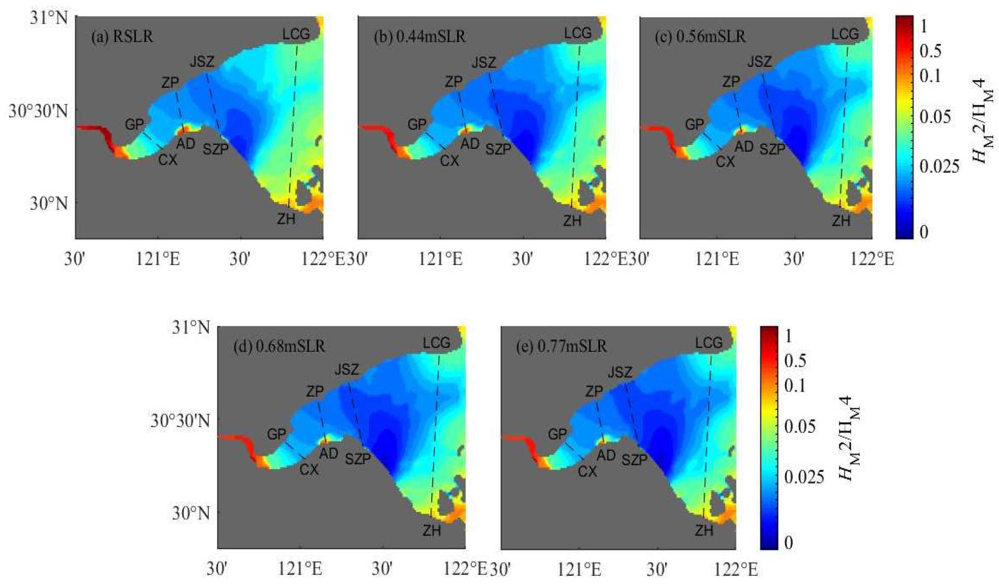
The ratio of the tidal amplitude plays a crucial role in determining the asymmetry. In the different SLR scenarios, the variations of the M₂ amplitude will significantly increase from the inner bay to the outer bay while the changes of the M₂ phase will be reduced by half from the inner bay to the outer bay. The SLR accelerates the propagation speed of the tidal waves, which will lead to the advance and increase the amplitude of M₂. However, the amplitude of M₄ decreases in the head bay. In the original inner and outer bays, the ratio started to increase from the surroundings to the middle area and gradually increased 0.01~0.02, particularly near the SZP area. In the end, the ratio firstly increases, then decreases and, finally, increases from west to east in relation to the topography, seabed friction and nonlinear dissipation of tidal waves. The main influence of the Coriolis force had an impact on the tide wave act toward the right, leading to the ratio of the north bank significantly greater than the south bank.

Our results showed the tidal asymmetry response to SLR in Hangzhou Bay, and a natural shallow basin provided a reliable numerical simulation. Eventually, a depth understanding the actual variety of the tidal response to the sea level rise in a real system has been proposed and thus provides insight into the impacts of the sea level rise, especially on the tidal asymmetry.

References

1. Blanton, J.O.; Francisco, A. Distortion of tidal currents and the lateral transfer of salt in a shallow coastal plain estuary (O estuário do Mira, Portugal). Estuaries 2001, 24, 467–480. [Google Scholar] [CrossRef]
2. Huang, H.; Chen, C.; Blanton, J.O.; Andrade, F.A. A numerical study of tidal asymmetry in Okatee Creek, South Carolina. Estuar. Coast. Shelf Sci. 2008, 78, 190–202. [Google Scholar] [CrossRef]
3. Savenije, H.H.G.; Veling, E.J.M. Relation between tidal damping and wave celerity in estuaries. J. Geophys. Res. Ocean. 2005, 110, C04007. [Google Scholar] [CrossRef] [Green Version]
4. Lu, S.; Tong, C.F.; Lee, D.Y.; Zheng, J.H.; Shen, J.; Zhang, W.; Yan, Y.X. Propagation of tidal waves up in Yangtze Estuary during the dry season. J. Geophys. Res. Ocean. 2015, 120, 6445–6473. [Google Scholar] [CrossRef] [Green Version]
5. Friedrichs, C.T.; Ole, S. Madsen Nonlinear diffusion of the tidal signal in frictionally dominated embayments. J. Geophys. Res. Ocean. 1992, 97, 5637–5650. [Google Scholar] [CrossRef]
6. Blanton, J.O.; Lin, G.; Elston, S.A. Tidal current asymmetry in shallow estuaries and tidal creeks. Cont. Shelf Res. 2002, 22, 1731–1743. [Google Scholar] [CrossRef]
7. Roshanka, R.; Charitha, P. Tidal inlet velocity asymmetry in diurnal regimes. Cont. Shelf Res. 2000, 20, 2347–2366. [Google Scholar] [CrossRef]
8. Elgar, S.; Guza, R.T. Observations of bispectra of shoaling surface gravity waves. J. Fluid Mech. 1985, 161, 425–448. [Google Scholar] [CrossRef]
9. Nidzieko, N.J.; Ralston, D.K. Tidal asymmetry and velocity skew over tidal flats and shallow channels within a macrotidal river delta. J. Geophys. Res. Ocean. 2012, 117, C03001. [Google Scholar] [CrossRef] [Green Version]
10. Song, D.H.; Wang, X.H.; Andrew, E.K.; Bao, X.W. The contribution to tidal asymmetry by different combinations of tidal constituents. J. Geophys. Res. Ocean. 2011, 116, C12007:1–C12007:12. [Google Scholar] [CrossRef]
11. Friedrichs, C.T.; Aubrey, D.G. Non-linear tidal distortion in shallow well-mixed estuaries: A synthesis. Estuar. Coast. Shelf Sci. 1988, 27, 521–545. [Google Scholar] [CrossRef]
12. Su, M.; Yao, P.; Wang, Z.B.; Zhang, C.K.; Stive, M.J.F. Tidal Wave Propagation in the Yellow Sea. J. Coast. Res. 2015, 57, 1550008. [Google Scholar] [CrossRef]
13. Lee, S.B.; Li, M.; Zhang, F. Impact of sea level rise on tidal range in Chesapeake and Delaware Bays. J. Geophys. Res. Ocean. 2017, 122, 3917–3938. [Google Scholar] [CrossRef]
14. Cai, H.Y.; Zhang, X.Y.; Zhang, M.; Guo, L.C.; Liu, F.; Yang, Q.S. Impacts of Three Gorges Dam’s operation on spatial–temporal patterns of tide–river dynamics in the Yangtze River estuary, China. Ocean Sci. 2019, 15, 583–599. [Google Scholar] [CrossRef] [Green Version]
15. Yu, Q.; Pan, H.D.; Gao, Y.Q.; Lv, X.Q. The Impact of the Mesoscale Ocean Variability on the Estimation of Tidal Harmonic Constants Based on Satellite Altimeter Data in the South China Sea. Remote Sens. 2021, 13, 2736. [Google Scholar] [CrossRef]
16. Pickering, M.D.; Horsburgh, K.J.; Blundell, J.R.; Hirschi, J.J.M.; Nicholls, R.J.; Verlaan, M.; Wells, N.C. The impact of future sea-level rise on the global tides. Cont. Shelf Res. 2017, 142, 50–68. [Google Scholar] [CrossRef] [Green Version]
17. Holly, E.; Pelling, J.A.; Mattias, G. Impact of flood defences and sea-level rise on the European Shelf tidal regime. Cont. Shelf Res. 2014, 85, 96–105. [Google Scholar]
18. Hui, F.; Xi, F.; Feng, W.B.; Zhang, W. Sensitivity of tides and tidal components to sea-level-rise in the Radial Sand Ridges. Reg. Stud. Mar. Sci. 2021, 47, 101918. [Google Scholar] [CrossRef]
19. Liang, H.D.; Kuang, C.P.; Maitane, O.; Gu, J.; Song, H.L.; Dong, Z.C. Coastal morphodynamic responses of a mixed-energy and fine-sediment coast to different sea level rise trends. Coast. Eng. 2020, 161, 103767. [Google Scholar] [CrossRef]
20. Benno, W.; Rita, S.; Caroline, R.; Frank, K. Tidal response to sea level rise and bathymetric changes in the German Wadden Sea. Ocean. Dynam. 2020, 70, 1033–1052. [Google Scholar] [CrossRef]
21. Cai, H.; Savenije, H.H.G.; Garel, E.; Zhang, X.; Guo, L.; Zhang, M.; Liu, F.; Yang, Q. Seasonal behaviour of tidal damping and residual water level slope in the Yangtze River estuary: Identifying the critical position and river discharge for maximum tidal damping. Hydrol. Earth. Syst. Sci. 2019, 23, 2779–2794. [Google Scholar] [CrossRef]
22. Chen, W.; Chen, K.; Kuang, C.P.; David, Z.Z.; He, L.L.; Mao, X.D.; Liang, H.D.; Song, H.L. Influence of sea level rise on saline water intrusion in the Yangtze River Estuary, China. Appl. Ocean Res. 2016, 54, 12–25. [Google Scholar] [CrossRef]
23. Fox-Kemper, B.; Hewitt, H.T.; Xiao, C.; Aðalgeirsdóttir, G.; Drijfhout, S.S.; Edwards, T.L.; Golledge, N.R.; Hemer, M.; Kopp, R.E.; Krinner, G.; et al. Ocean, cryosphere and sea level change. In Climate Change 2021: The Physical Science Basis; Cambridge University Press: Cambridge, UK, 2021; in press. [Google Scholar]
24. Allan, R.P.; Arias, P.A.; Berger, S.; Canadell, J.G.; Cassou, C.; Chen, D.; Cherchi, A.; Connors, S.L.; Coppola, E.; Cruz, F.A.; et al. Climate Change 2021: The physical Science Basis. Contribution of Working Group I to the Sixth Assessment Report of the Intergovernmental Panel on Climate Change; Cambridge University Press: Cambridge, UK, 2021; in press. [Google Scholar]
25. Hermans, T.H.J.; Tinker, J.; Palmer, M.D.; Katsman, C.A.; Vermeersen, B.L.A.; Slangen, A.B.A. Improving sea-level projections on the Northwestern European shelf using dynamical downscaling. Clim. Dyn. 2020, 54, 1987–2011. [Google Scholar] [CrossRef] [Green Version]
26. Hermans, T.H.J.; Gregory, J.M.; Palmer, M.D.; Ringer, M.A.; Katsman, C.A.; Slangen, A.B.A. Projecting Global Mean Sea-Level Change Using CMIP6 Models. Geophys. Res. Lett. 2021, 48, e2020GL092064. [Google Scholar] [CrossRef]
27. Du, Y.F.; Wang, D.S.; Zhang, J.C.; Wang, Y.P.; Fan, D.D. Estimation of initial conditions for surface suspended sediment simulations with the adjoint method: A case study in Hangzhou Bay. Cont. Shelf Res. 2021, 227, 104526. [Google Scholar] [CrossRef]
28. Li, Y.D.; Li, X.F. Remote sensing observations and numerical studies of a super typhoon-induced suspended sediment concentration variation in the East China Seat. Ocean Model. 2016, 104, 187–202. [Google Scholar] [CrossRef]
29. Feng, L.; He, J.; Ai, J.G.; Sun, X.; Bian, F.Y.; Zhu, X.D. Evaluation for coastal reclamation feasibility using a comprehensive hydrodynamic framework: A case study in Haizhou Bay. Mar. Pollut. Bull. 2015, 100, 182–190. [Google Scholar] [CrossRef]
30. Casulli, V.; Walters, R.A. An unstructured grid, three-dimensional model based on the shallow water equations. Int. J. Numer. Meth. Fluids 2000, 32, 331–348. [Google Scholar] [CrossRef]
31. Chen, W.B.; Liu, W.C. Modeling investigation of asymmetric tidal mixing and residual circulation in a partially stratified estuary. Environ. Fluid Mech. 2016, 16, 167–191. [Google Scholar] [CrossRef]
32. Ye, T.Y. The Multi-Scale Variations of Suspended Sediment Dynamics in Hangzhou Bay and Its Interaction with Tidal Flat Variations; Zhejiang University: Zhoushan, China, 2019; pp. 48–54, (In Chinese). [Google Scholar] [CrossRef]
33. Cai, H.Y.; Zhang, P.; Garel, E.; Matte, P.; Hu, S.; Liu, F.; Yang, Q.S. A novel approach for the assessment of morphological evolution based on observed water levels in tide-dominated estuaries. Hydrol. Earth. Syst. Sci. 2020, 24, 1871–1889. [Google Scholar] [CrossRef]
34. Li, L.; Ye, T.Y.; He, Z.G.; Xia, Y.Z. A numerical study on the effect of tidal flat’s slope on tidal dynamics in the Xiangshan Bay, China. Acta Oceanol. Sin. 2018, 37, 29–40. [Google Scholar] [CrossRef]
35. Pugh, D.T. Tides, Surges and Mean Sea-Level; John Wiley & Sons: New York, NY, USA, 1987; 472p. [Google Scholar]
36. Wu, R.H.; Jiang, Z.T.; Li, C.Y. Revisiting the tidal dynamics in the complex Zhoushan Archipelago waters: A numerical experimentt. Ocean Model. 2018, 132, 139–156. [Google Scholar] [CrossRef]
37. Yu, M.G. A preliminary discussion on the tidal characteristics of the South China Sea. Acta Oceanol. Sin. 1984, 3, 293–300. (In Chinese) [Google Scholar]
38. Nidzieko, N.J. Tidal asymmetry in estuaries with mixed semidiurnal/diurnal tides. J. Geophys. Res. Earth Surf. 2010, 115, C08006. [Google Scholar] [CrossRef] [Green Version]
39. Blanton, J.O.; Tenore, K.R.; Castillejo, F.; Atkinson, L.P.; Schwing, F.B.; Lavin, A. The relationship of upwelling to mussel production in the rias on the western coast of Spain. J. Mar. Res. 1987, 45, 497–511. [Google Scholar] [CrossRef] [Green Version]
40. Zarzuelo, C.; D’Alpaos, A.; Carniello, L.; López-Ruiz, A.; Díez-Minguito, M.; Ortega-Sánchez, M. Natural and Human-Induced Flow and Sediment Transport within Tidal Creek Networks Influenced by Ocean-Bay Tides. Water 2019, 11, 1493. [Google Scholar] [CrossRef] [Green Version]
41. Bian, C.W.; Jiang, W.S.; Song, D.H. Terrigenous transportation to the Okinawa Trough and the influence of typhoons on suspended sediment concentration. Cont. Shelf Res. 2010, 30, 1189–1199. [Google Scholar] [CrossRef]
42. Chu, D.D.; Niu, H.B.; Wang, Y.P.; Cao, A.Z.; Li, L.; Du, Y.F.; Zhang, J.C. Numerical study on tidal duration asymmetry and shallow-water tides within multiple islands: An example of the Zhoushan Archipelago. Estuar. Coast. Shelf Sci. 2021, 262, 107576. [Google Scholar] [CrossRef]
43. Lafta, A. Investigation of tidal asymmetry in the Shatt Al-Arab river estuary, Northwest of Arabian Gulf. Oceanologia 2022, 64, 376–386. [Google Scholar] [CrossRef]
44. LeBlond, P.H. On tidal propagation in shallow rivers. J. Geophys. Res. Ocean. 1978, 83, 4717–4721. [Google Scholar] [CrossRef]
45. Speer, P.E.; Aubrey, D.G. A study of non-linear tidal propagation in shallow inlet/estuarine systems Part II: Theory. Estuar. Coast. Shelf Sci. 1985, 21, 207–224. [Google Scholar] [CrossRef]
46. Speer, P.E.; Aubrey, D.G.; Friedrichs, C.T. Nonlinear hydrodynamics of shallow tidal inlet/bay systems. Tidal Hydrodyn. 1991, 321, 339. [Google Scholar]
47. Davies, A.M.; Lawrence, J. Modelling the non-linear interaction of wind and tide: Its influence on current profiles. Int. J. Numer. Meth. Fluids 1994, 18, 163–188. [Google Scholar] [CrossRef]
48. Elgar, S.; Herbers, T.H.C.; Guza, R.T. Reflection of ocean surface gravity waves from a natural beach. J. Phys. Oceanogr. 1994, 24, 1503–1511. [Google Scholar] [CrossRef]
49. Guo, L.C.; Xu, F.; Mick, W.; Townend, I.; Wang, Z.B.; He, Q. Morphodynamic adaptation of a tidal basin to centennial sea-level rise: The importance of lateral expansion. Cont. Shelf Res. 2021, 226, 104494. [Google Scholar] [CrossRef]
50. Ma, J.Y.; Guo, D.Q.; Zhan, P.; Hoteit, I. Seasonal M2 Internal Tides in the Arabian Sea. Remote Sens. 2021, 13, 2823. [Google Scholar] [CrossRef]
Figure 1. (a) Location map of the study area showing the large-scale Hangzhou Bay model of three stations of Datong, Jiangyin and Cangqian. (b) Domain of the Hangzhou Bay model showing the depth and location of the tidal gauges for the tide level (black dots) and tidal current (red dots).
Jmse 10 01445 g001
Figure 2. Time series of the hourly tide level records along Hangzhou Bay at the GP (a) and ZP (b) stations during September 2010.
Jmse 10 01445 g002
Figure 3. Comparison of the time series of the tidal velocity (a,c,e,g,i,k,m,o) and direction (b,d,f,h,j,l,n,p) at four tidal gauges of the spring tide (S) and neap tide (N) during September 2010.
Jmse 10 01445 g003
Figure 4. The water depth at the Hangzhou Bay stations (H1–H20) and the point of the distribution of skewness from June to September 2020.
Jmse 10 01445 g004
Figure 5. The point of (Figure 4) the variation of skewness along Hangzhou Bay for different SLR scenarios, SLR-induced skewness changes under (a) H1–H5, (b) H6–10, (c) H11–15 and (d) H16–H20, respectively.
Jmse 10 01445 g005
Figure 6. SLR-induced tidal range changes under (a) 0.44 m SLR, (b) 0.56 m SLR, (c) 0.68 m SLR and (d) 0.77 m SLR, which are calculated by the tidal ranges in different sea level scenarios minus that in the RSLR.
Jmse 10 01445 g006
Figure 7. Differences in the (ad) M2 amplitude and (eh) M2 phase between the SLR scenarios and RSLR scenario.
Jmse 10 01445 g007
Figure 8. The ratio of the H M 2 / H M 4 variations under (a) RSLR, (b) 0.44 m SLR, (c) 0.56 m SLR, (d) 0.68 m SLR and (e) 0.77 m SLR in the Hangzhou Bay model.
Jmse 10 01445 g008