
An Improved Approach to Wave Energy Resource Characterization for Sea States with Multiple Wave Systems

Abstract
:1. Introduction
2. Materials and Methods
2.1. Modeling of Long Time Series Wave Spectra
2.2. Partitioning and Grouping Procedure
2.3. Characteristic Parameters of Wave Energy
- Wave spectra and spectral moments
- 2.
- Significant wave height and wave energy period
- 3.
- Omnidirectional wave energy flux
- 4.
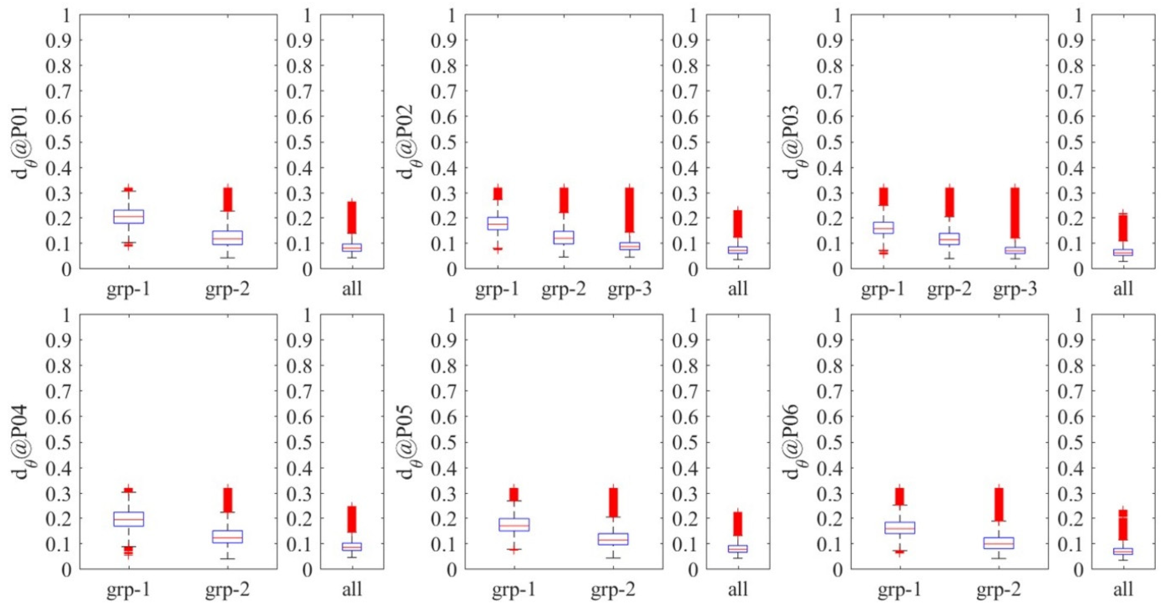
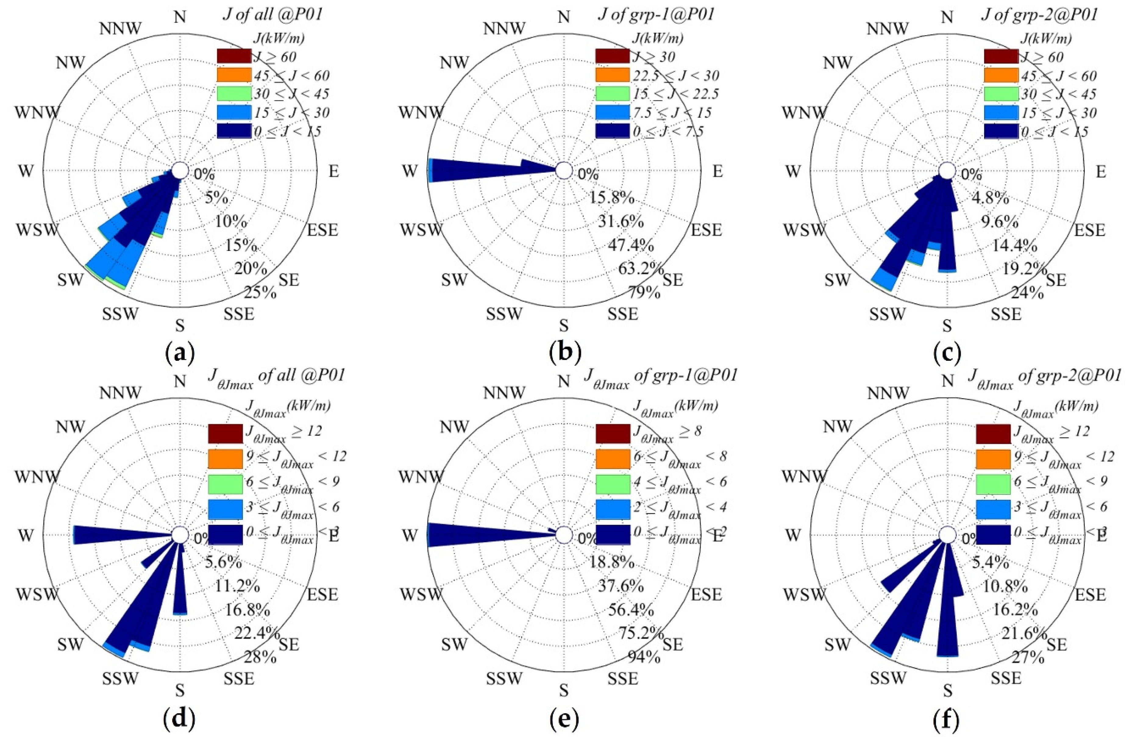
- Directionally resolved wave energy flux
- 5.
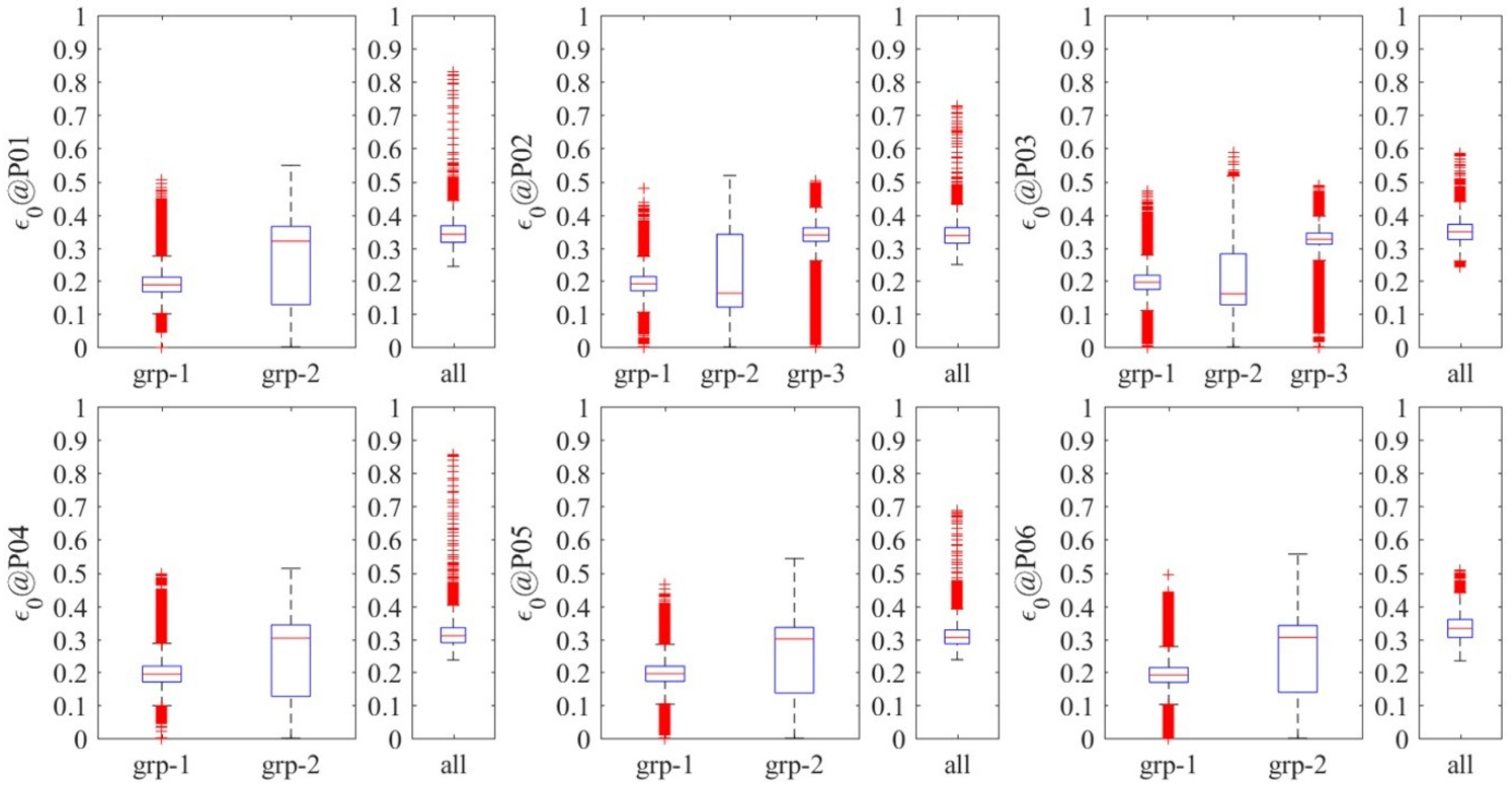
- Spectral width
- 6.
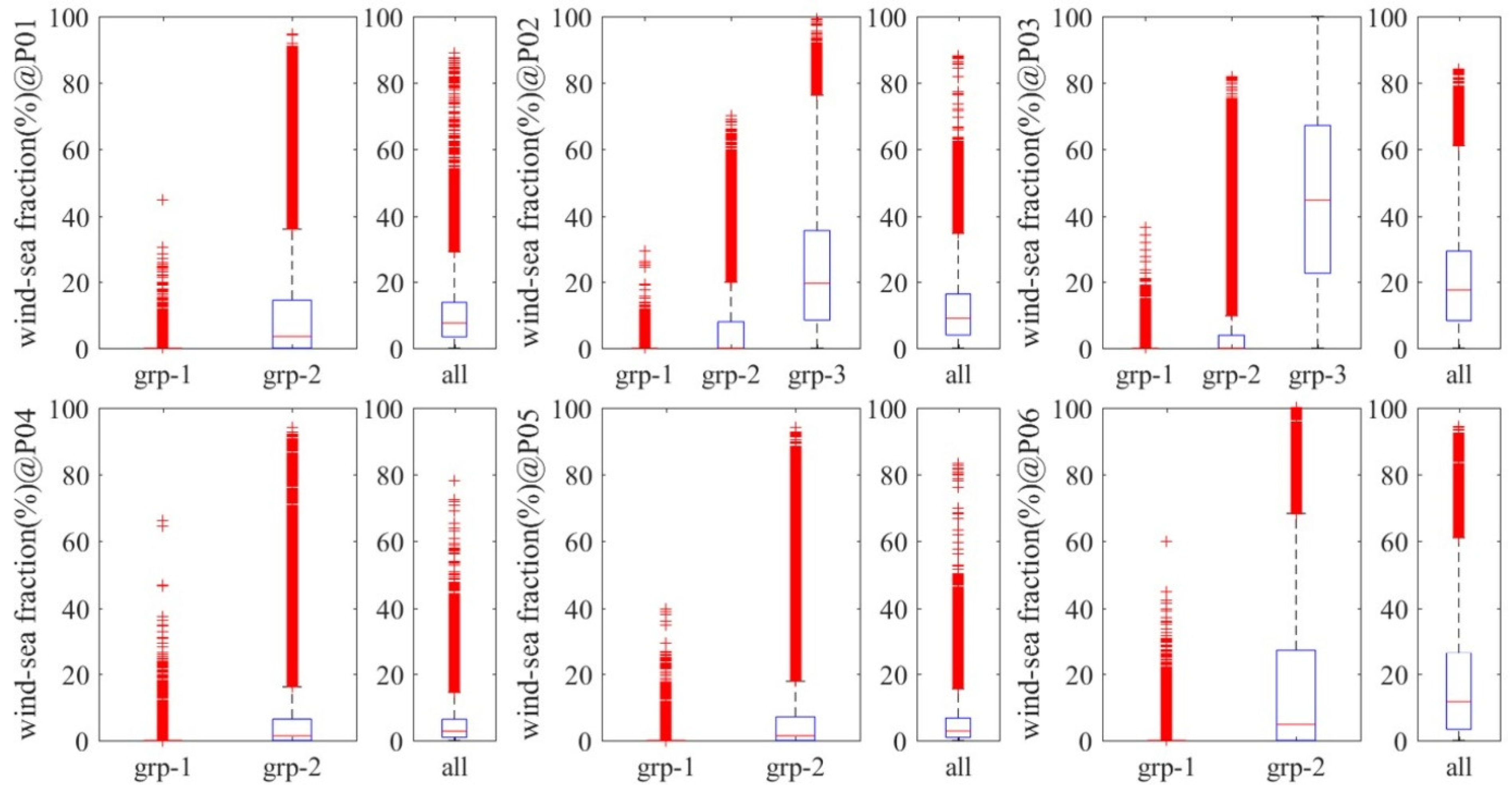
- Wind-sea fraction
3. Results
3.1. Wave System Groups
3.2. Wind Wave and Swell Contributions to Wave Energy
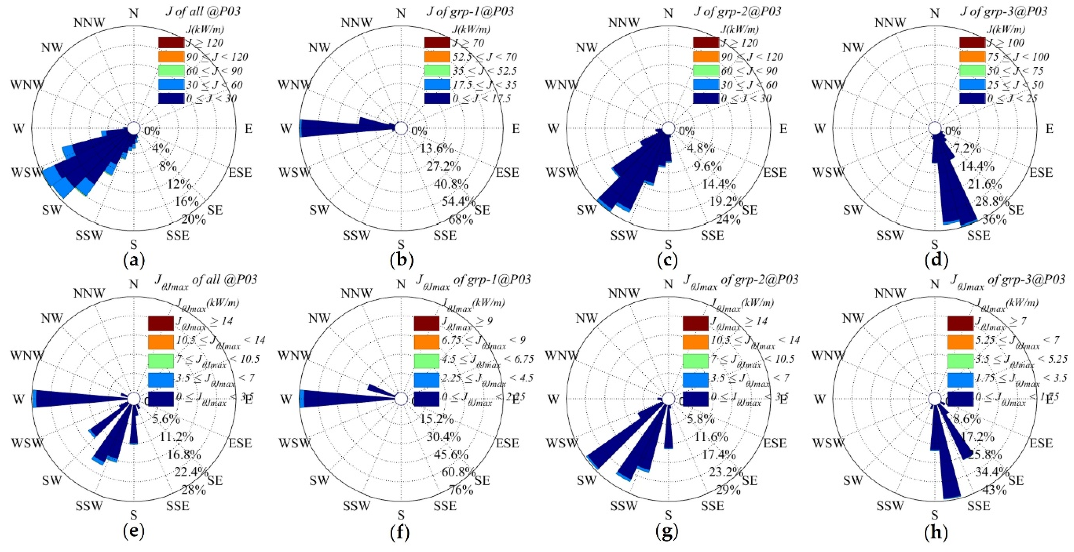
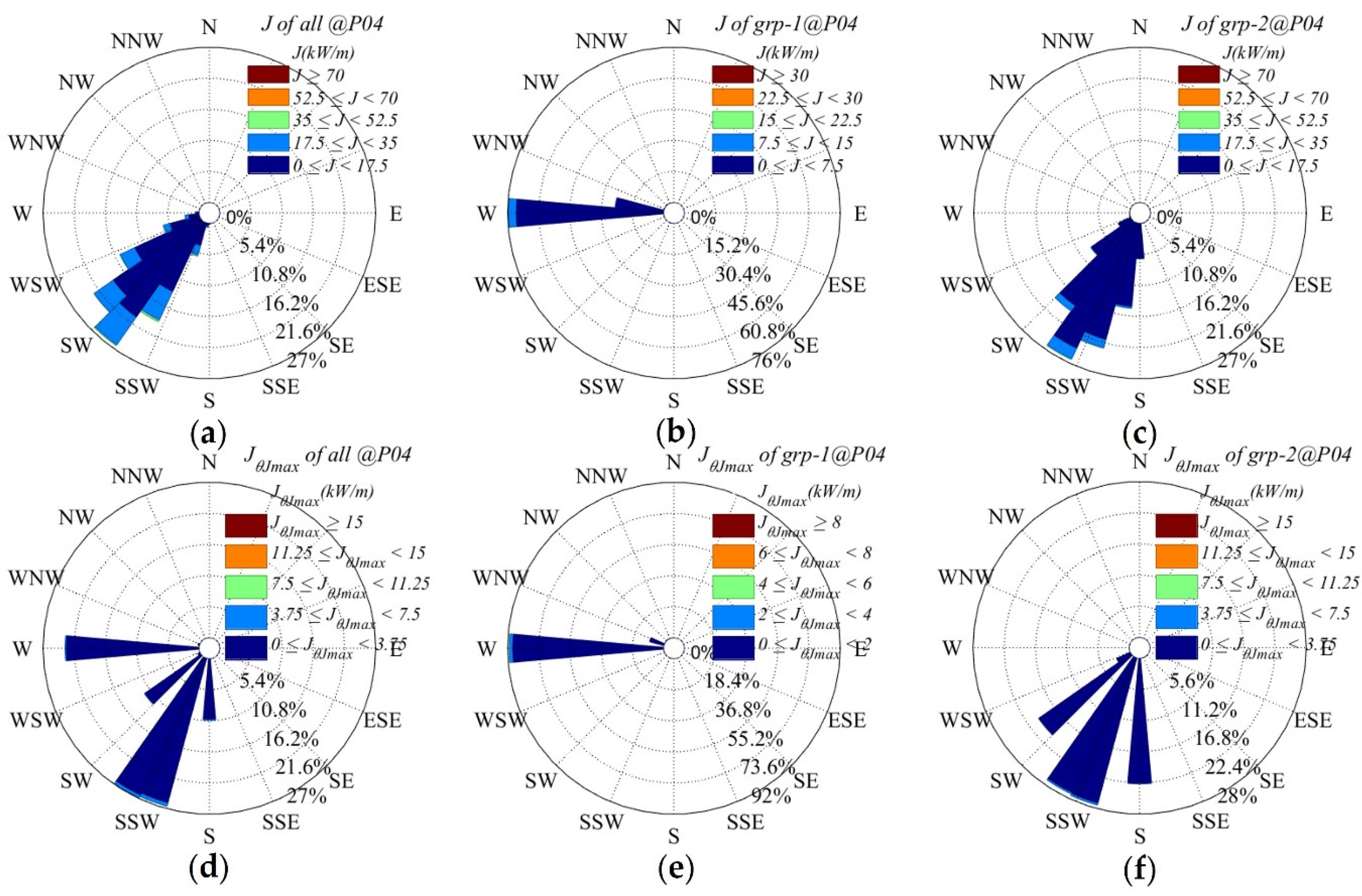
3.3. Directionality
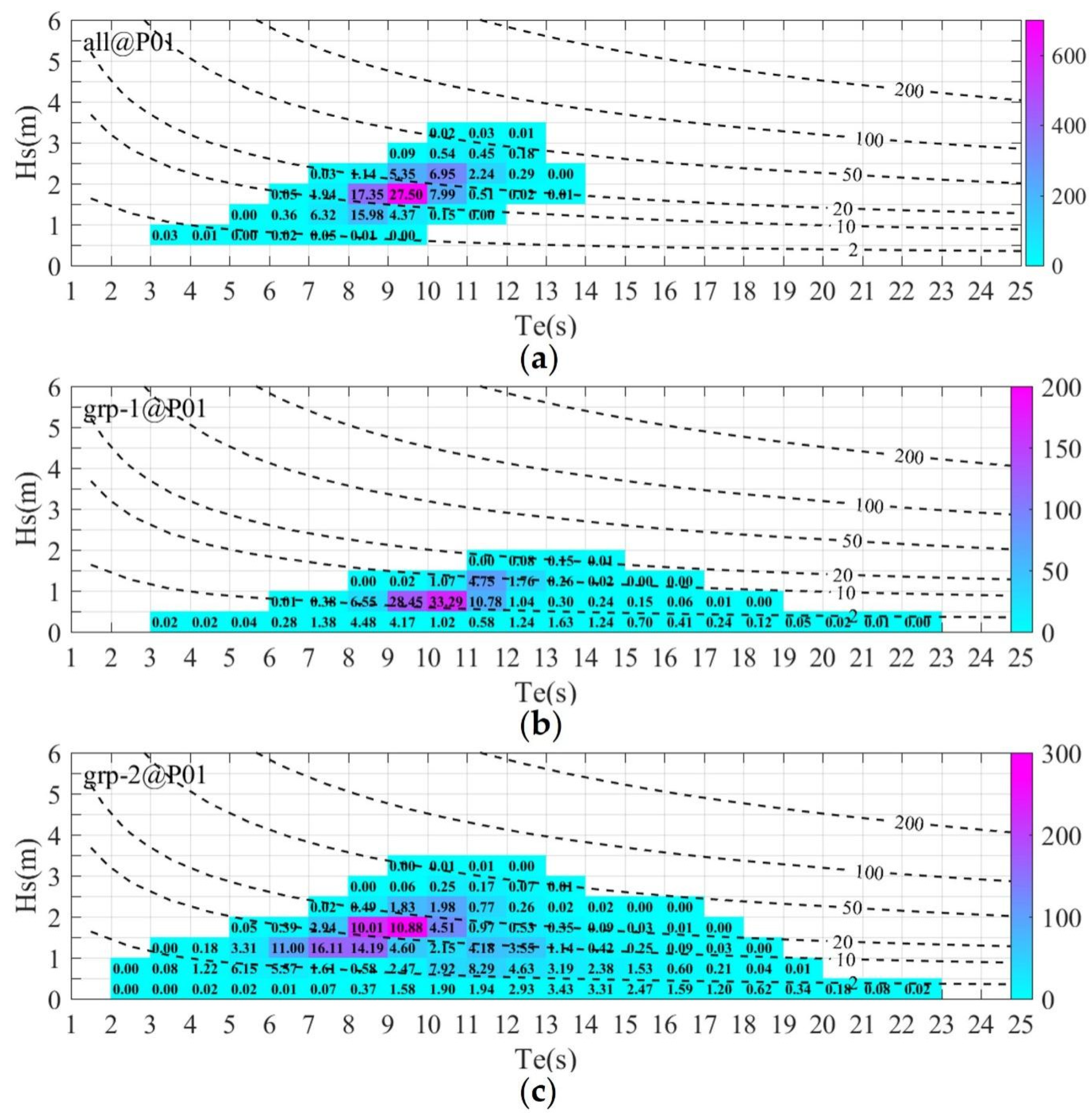
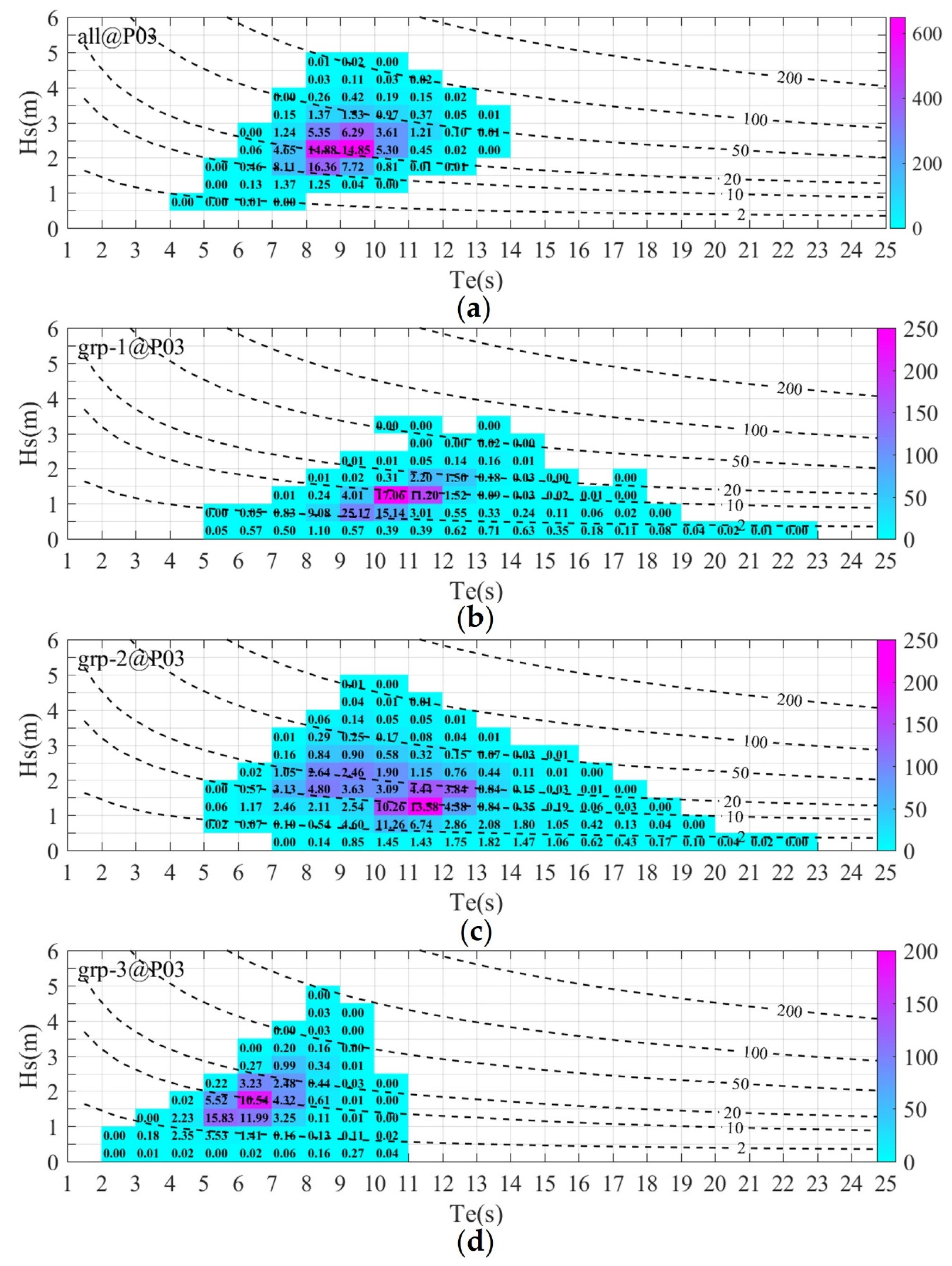
3.4. Wave Conditions
4. Discussion
5. Conclusions
Author Contributions
Funding
Institutional Review Board Statement
Informed Consent Statement
Data Availability Statement
Acknowledgments
Conflicts of Interest
References
- Pelc, R.; Fujita, R.M. Renewable energy from the ocean. Mar. Policy 2002, 26, 471–479. [Google Scholar] [CrossRef]
- Zheng, C.; Pan, J.; Li, J. Assessing the China Sea wind energy and wave energy resources from 1988 to 2009. Ocean Eng. 2013, 65, 39–48. [Google Scholar] [CrossRef]
- Zheng, C.; Shao, L.; Shi, W.; Su, Q.; Lin, G.; Li, X.; Chen, X. An assessment of global ocean wave energy resources over the last 45 a. Acta Oceanol. Sin. 2014, 33, 92–101. [Google Scholar] [CrossRef]
- Kamranzad, B.; Etemad-Shahidi, A.; Chegini, V. Developing an optimum hotspot identifier for wave energy extracting in the northern Persian Gulf. Renew. Energy 2017, 114, 59–71. [Google Scholar] [CrossRef]
- Rusu, E.; Onea, F. Estimation of the wave energy conversion efficiency in the Atlantic Ocean close to the European islands. Renew. Energy 2016, 85, 687–703. [Google Scholar] [CrossRef]
- Silva, D.; Rusu, E.; Soares, C. Evaluation of Various Technologies for Wave Energy Conversion in the Portuguese Nearshore. Energies 2013, 6, 1344–1364. [Google Scholar] [CrossRef]
- Rusu, L.; Onea, F. Assessment of the performances of various wave energy converters along the European continental coasts. Energy 2015, 82, 889–904. [Google Scholar] [CrossRef]
- Rusu, L.; Onea, F. The performance of some state-of-the-art wave energy converters in locations with the worldwide highest wave power. Renew. Sustain. Energy Rev. 2017, 75, 1348–1362. [Google Scholar] [CrossRef]
- Vaquero, A.; Ruiz, F.; Rusu, E. Evaluation of the wave power potential in the northwestern side of the Iberian nearshore. In Developments in Maritime Transportation and Exploitation of Sea Resources; CRC Press: Boca Raton, FL, USA, 2013; pp. 1011–1019. ISBN 9781482233001. [Google Scholar]
- Saulnier, J.-B.; Clément, A.; Falcão, A.F.d.O.; Pontes, T.; Prevosto, M.; Ricci, P. Wave groupiness and spectral bandwidth as relevant parameters for the performance assessment of wave energy converters. Ocean Eng. 2011, 38, 130–147. [Google Scholar] [CrossRef]
- Marquis, L.; Kramer, M.; Frigaard, P. First Power Production figures from the Wave Star Roshage Wave Energy Converter. In Proceedings of the 3rd International Conference on Ocean Energy, Bilbao, Spain, 6 October 2010; pp. 1–5. [Google Scholar]
- Pelamis, World’s First Commercial Wave Energy Project, Agucadoura—Power Technology. Available online: http://www.power-technology.com/projects/pelamis/ (accessed on 17 February 2022).
- Kofoed, J.P.; Frigaard, P.; Friis-Madsen, E.; Sørensen, H.C. Prototype testing of the wave energy converter wave dragon. Renew. Energy 2006, 31, 181–189. [Google Scholar] [CrossRef] [Green Version]
- Babarit, A.; Hals, J.; Muliawan, M.J.; Kurniawan, A.; Moan, T.; Krokstad, J. Numerical benchmarking study of a selection of wave energy converters. Renew. Energy 2012, 41, 44–63. [Google Scholar] [CrossRef]
- Weinstein, A.; Fredrikson, G.; Parks, M.J.; Nielsen, K. AquaBuOY—The offshore wave energy converter numerical modeling and optimization. In Proceedings of the Oceans ’04 MTS/IEEE Techno-Ocean ’04 (IEEE Cat. No.04CH37600), Kobe, Japan, 9–12 November 2004; Volume 4, pp. 1854–1859. [Google Scholar]
- Tavakoli, S.; Babanin, A.V. Wave energy attenuation by drifting and non-drifting floating rigid plates. Ocean Eng. 2021, 226, 108717. [Google Scholar] [CrossRef]
- Patel, R.P.; Nagababu, G.; Kachhwaha, S.S.; Kumar, S.V.A.; Seemanth, M. Combined wind and wave resource assessment and energy extraction along the Indian coast. Renew. Energy 2022, 195, 931–945. [Google Scholar] [CrossRef]
- Orejarena-Rondón, A.F.; Restrepo, J.C.; Correa-Metrio, A.; Orfila, A. Wave energy flux in the Caribbean Sea: Trends and variability. Renew. Energy 2022, 181, 616–629. [Google Scholar] [CrossRef]
- Vieira, F.; Cavalcante, G.; Campos, E.; Taveira-Pinto, F. Wave energy flux variability and trend along the United Arab Emirates coastline based on a 40-year hindcast. Renew. Energy 2020, 160, 1194–1205. [Google Scholar] [CrossRef]
- Ahn, S.; Neary, V.S.; Allahdadi, M.N.; He, R. Nearshore wave energy resource characterization along the East Coast of the United States. Renew. Energy 2021, 172, 1212–1224. [Google Scholar] [CrossRef]
- Rusu, L. A projection of the expected wave power in the Black Sea until the end of the 21st century. Renew. Energy 2020, 160, 136–147. [Google Scholar] [CrossRef]
- Ribal, A.; Babanin, A.V.; Zieger, S.; Liu, Q. A high-resolution wave energy resource assessment of Indonesia. Renew. Energy 2020, 160, 1349–1363. [Google Scholar] [CrossRef]
- Lokuliyana, R.L.K.; Folley, M.; Gunawardane, S.D.G.S.P.; Wickramanayake, P.N. Sri Lankan wave energy resource assessment and characterisation based on IEC standards. Renew. Energy 2020, 162, 1255–1272. [Google Scholar] [CrossRef]
- Jahangir, M.H.; Mazinani, M. Evaluation of the convertible offshore wave energy capacity of the southern strip of the Caspian Sea. Renew. Energy 2020, 152, 331–346. [Google Scholar] [CrossRef]
- IEC Part 101: Wave energy resource assessment and characterization. In Marine Energy—Wave, Tidal and Other Water Current Converters; BSI Standards Limited: London, UK, 2015; ISBN 978 0 580 79774 3.
- Mediavilla, D.G.; Figueroa, D. Assessment, sources and predictability of the swell wave power arriving to Chile. Renew. Energy 2017, 114, 108–119. [Google Scholar] [CrossRef]
- Kerbiriou, M.; Prevosto, M.; Maisondieu, C.; Clement, A.; Babarit, A. Influence of Sea-States Description on Wave Energy Production Assessment. In Proceedings of the 7th European Wave and Tidal Energy Conference, Porto, Portugal, 11–13 September 2007. [Google Scholar]
- Zheng, C. Global oceanic wave energy resource dataset—With the Maritime Silk Road as a case study. Renew. Energy 2021, 169, 843–854. [Google Scholar] [CrossRef]
- Li, N.; García-Medina, G.; Cheung, K.F.; Yang, Z. Wave energy resources assessment for the multi-modal sea state of Hawaii. Renew. Energy 2021, 174, 1036–1055. [Google Scholar] [CrossRef]
- Forristall, G.Z.; Ewans, K.; Olagnon, M.; Prevosto, M. The West Africa Swell Project (WASP). In Proceedings of the ASME 2013 32nd International Conference on Ocean, Offshore and Arctic Engineering, Nantes, France, 9–14 June 2013. [Google Scholar]
- Prevosto, M.; Ewans, K.; Forristall, G.Z.; Olagnon, M. Swell Genesis, Modelling and Measurements in West Africa. In Proceedings of the AMSE 2013 32nd International Conference on Ocean, Offshore and Arctic Engineering, Nantes, France, 9–14 June 2013. [Google Scholar]
- Olagnon, M.; Ewans, K.; Forristall, G.; Prevosto, M. West Africa Swell Spectral Shapes. In Proceedings of the AMSE 2013 32nd International Conference on Ocean, Offshore and Arctic Engineering, Nantes, France, 9–14 June 2013. [Google Scholar]
- Stone, R.G.; Riehl, H. Tropical Meteorology. Geogr. Rev. 1956, 46, 448. [Google Scholar] [CrossRef]
- Byers, H.R.; Landsberg, H.E.; Wexler, H.; Haurwitz, B.; Spilhaus, A.F.; Willett, H.C.; Houghton, H.G. Compendium of Meteorology; Malone, T.F., Ed.; American Meteorological Society: Boston, MA, USA, 1951; ISBN 978-1-940033-70-9. [Google Scholar]
- Booij, N.; Ris, R.C.; Holthuijsen, L.H. A third-generation wave model for coastal regions: 1. Model description and validation. J. Geophys. Res. Oceans 1999, 104, 7649–7666. [Google Scholar] [CrossRef]
- Ris, R.C.; Holthuijsen, L.H.; Booij, N. A third-generation wave model for coastal regions: 2. Verification. J. Geophys. Res. Oceans 1999, 104, 7667–7681. [Google Scholar] [CrossRef]
- Tolman, H.L. The Numerical Model WAVEWATCH; Delft Univ. of Techn.: Delft, The Netherlands, 1989. [Google Scholar]
- Tolman, H.L. A Third-Generation Model for Wind Waves on Slowly Varying, Unsteady, and Inhomogeneous Depths and Currents. J. Phys. Oceanogr. 1991, 21, 782–797. [Google Scholar] [CrossRef]
- Tolman, H.L.; Chalikov, D. Source Terms in a Third-Generation Wind Wave Model. J. Phys. Oceanogr. 1996, 26, 2497–2518. [Google Scholar] [CrossRef]
- Yuan, Y.; Hua, F.; Pan, Z.; Sun, L. LAGDF-WAM numerical wave model—I. basic physical model. Acta Oceanol. Sin. 1991, 10, 483–488. [Google Scholar]
- Yuan, Y.; Hua, F.; Pan, Z.; Sun, L. LAGFD-WAM numerical wave model—II: Characteristics inlaid scheme and its application. Acta Oceanol. Sin. 1992, 11, 13–23. [Google Scholar]
- Yang, Y.; Qiao, F.; Zhao, W.; Teng, Y.; Yuan, Y. MASNUM ocean wave numerical model in spherical coordinates and its application. Acta Oceanol. Sin. 2005, 27, 1–7. [Google Scholar]
- Yuan, Y.; Tung, C.C.; Huang, N.E. Statistical Characteristics of Breaking Waves. In Wave Dynamics and Radio Probing of the Ocean Surface; Springer US: Boston, MA, USA, 1986; pp. 265–272. [Google Scholar]
- Snyder, R.L.; Dobson, F.W.; Elliott, J.A.; Long, R.B. Array measurements of atmospheric pressure fluctuations above surface gravity waves. J. Fluid Mech. 1981, 102, 1–59. [Google Scholar] [CrossRef]
- Hasselmann, S.; Hasselmann, K. Computations and Parameterizations of the Nonlinear Energy Transfer in a Gravity-Wave Specturm. Part II: Parameterizations of the Nonlinear Energy Transfer for Application in Wave Models. J. Phys. Oceanogr. 1985, 15, 1378–1391. [Google Scholar] [CrossRef]
- Hasselmann, S.; Hasselmann, K. Computations and Parameterizations of the Nonlinear Energy Transfer in a Gravity-Wave Spectrum. Part I: A New Method for Efficient Computations of the Exact Nonlinear Transfer Integral. J. Phys. Oceanogr. 1985, 15, 1369–1377. [Google Scholar] [CrossRef]
- Bao, Y.; Song, Z.; Qiao, F. FIO-ESM Version 2.0: Model Description and Evaluation. J. Geophys. Res. Oceans 2020, 125, e2019JC016036. [Google Scholar] [CrossRef]
- Sun, M.; Yin, X.; Yang, Y.; Wu, K. An effective method based on dynamic sampling for data assimilation in a global wave model. Ocean Dyn. 2017, 67, 433–449. [Google Scholar] [CrossRef]
- Jiang, B.; Wei, Y.; Jiang, X.; Wang, H.; Wang, X.; Ding, J.; Zhang, R.; Shi, Y.; Cai, X.; Wu, Y. Assessment of wave energy resource of the Bohai Sea, Yellow Sea and East China Sea based on 10-year numerical hindcast data. In Proceedings of the OCEANS 2016—Shanghai, Shanghai, China, 10–13 April 2016; pp. 1–9. [Google Scholar]
- Jiang, X.; Wang, D.; Gao, D.; Zhang, T. Experiments on exactly computing non-linear energy transfer rate in MASNUM-WAM. Chin. J. Oceanol. Limnol. 2016, 34, 821–834. [Google Scholar] [CrossRef]
- Wang, G.; Zhao, C.; Xu, J.; Qiao, F.; Xia, C. Verification of an operational ocean circulation-surface wave coupled forecasting system for the China’s seas. Acta Oceanol. Sin. 2016, 35, 19–28. [Google Scholar] [CrossRef]
- Qiao, F.; Wang, G.; Khokiattiwong, S.; Akhir, M.F.; Zhu, W.; Xiao, B. China published ocean forecasting system for the 21st-Century Maritime Silk Road on December 10, 2018. Acta Oceanol. Sin. 2019, 38, 1–3. [Google Scholar] [CrossRef]
- Hasselmann, K.; Barnett, T.P.; Bouws, E.; Carlson, H.; Cartwright, D.E.; Eake, K.; Euring, J.A.; Gicnapp, A.; Hasselmann, D.E.; Kruseman, P.; et al. Measurements of wind-wave growth and swell decay during the joint North Sea wave project (JONSWAP). Ergnzungsheft Dtsch. Hydrogr. Z. Reihe 1973, A, 95. [Google Scholar]
- Wessel, P.; Smith, W.H.F. A global, self-consistent, hierarchical, high-resolution shoreline database. J. Geophys. Res. Solid Earth 1996, 101, 8741–8743. [Google Scholar] [CrossRef]
- Vincent, L.; Soille, P. Watersheds in Digital Spaces: An Efficient Algorithm Based on Immersion Simulations. IEEE Trans. Pattern Anal. Mach. Intell. 1991, 13, 583–598. [Google Scholar] [CrossRef]
- Hasselmann, S.; Brüning, C.; Hasselmann, K.; Heimbach, P. An improved algorithm for the retrieval of ocean wave spectra from synthetic aperture radar image spectra. J. Geophys. Res. Oceans 1996, 101, 16615–16629. [Google Scholar] [CrossRef]
- Hanson, J.L.; Phillips, O.M. Automated Analysis of Ocean Surface Directional Wave Spectra. J. Atmos. Ocean. Technol. 2001, 18, 277–293. [Google Scholar] [CrossRef]
- Young, I.R.; Glowacki, T.J. Assimilation of altimeter wave height data into a spectral wave model using statistical interpolation. Ocean Eng. 1996, 23, 667–689. [Google Scholar] [CrossRef]
- Voorrips, A.C.; Makin, V.K.; Hasselmann, S. Assimilation of wave spectra from pitch-and-roll buoys in a North Sea wave model. J. Geophys. Res. Oceans 1997, 102, 5829–5849. [Google Scholar] [CrossRef]
- Devaliere, E.-M.; Hanson, J.L.; Luettich, R. Spatial Tracking of Numerical Wave Model Output Using a Spiral Search Algorithm. In Proceedings of the 2009 WRI World Congress on Computer Science and Information Engineering, Los Angeles, CA, USA, 31 March–2 April 2009; pp. 404–408. [Google Scholar]
- Portilla-Yandún, J.; Salazar, A.; Cavaleri, L. Climate patterns derived from ocean wave spectra. Geophys. Res. Lett. 2016, 43, 11–736. [Google Scholar] [CrossRef]
- Portilla-Yandún, J.; Cavaleri, L.; Van Vledder, G.P. Wave spectra partitioning and long term statistical distribution. Ocean Model. 2015, 96, 148–160. [Google Scholar] [CrossRef]
- Portilla-Yandún, J.; Barbariol, F.; Benetazzo, A.; Cavaleri, L. On the statistical analysis of ocean wave directional spectra. Ocean Eng. 2019, 189, 106361. [Google Scholar] [CrossRef]
- WAVEWATCH-III.v6.07 Release. Available online: https://github.com/NOAA-EMC/WW3/releases/tag/6.07 (accessed on 21 September 2022).
- Hanson, J.L.; Jensen, R.E. Wave system diagnostics for numerical wave models. In Proceedings of the 8 th International Workshop on Wave Hindcasting and Forecasting, Oahu, HI, USA, 11–14 November 2004. [Google Scholar]
- Hanson, J.L.; Tracy, B.A.; Tolman, H.L.; Scott, R.D. Pacific Hindcast Performance of Three Numerical Wave Models. J. Atmos. Ocean. Technol. 2009, 26, 1614–1633. [Google Scholar] [CrossRef]
- Tracy, B.; Devaliere, E.; Hanson, J.; Nicolini, T.; Tolman, H. Wind Sea and Swell Delineation for Numerical Wave Modeling. In Proceedings of the 10th International Workshop on Wave Hindcasting and Forecasting Coastal Hazard Symposium, Oahu, HI, USA, 11–16 November 2007; p. 12. [Google Scholar]
- The WAVEWATCH III R Development Group. User Manual and System Documentation of WAVEWATCH III R Version 5.16; NOAA/NCEP: College Park, MD, USA, 2016. [Google Scholar]
- Langford, E. Quartiles in Elementary Statistics. J. Stat. Educ. 2006, 14. [Google Scholar] [CrossRef]
- Nelson, L.S. Evaluating Overlapping Confidence Intervals. J. Qual. Technol. 1989, 21, 140–141. [Google Scholar] [CrossRef]
- Radford, P.J.; Velleman, P.F.; Hoaglin, D.C. Applications, Basics, and Computing of Exploratory Data Analysis. Biometrics 1983, 39, 815. [Google Scholar] [CrossRef]
- Mcgill, R.; Tukey, J.W.; Larsen, W.A. Variations of Box Plots. Am. Stat. 1978, 32, 12–16. [Google Scholar]
- Liwen Bianji. Available online: https://www.liwenbianji.cn (accessed on 21 September 2022).


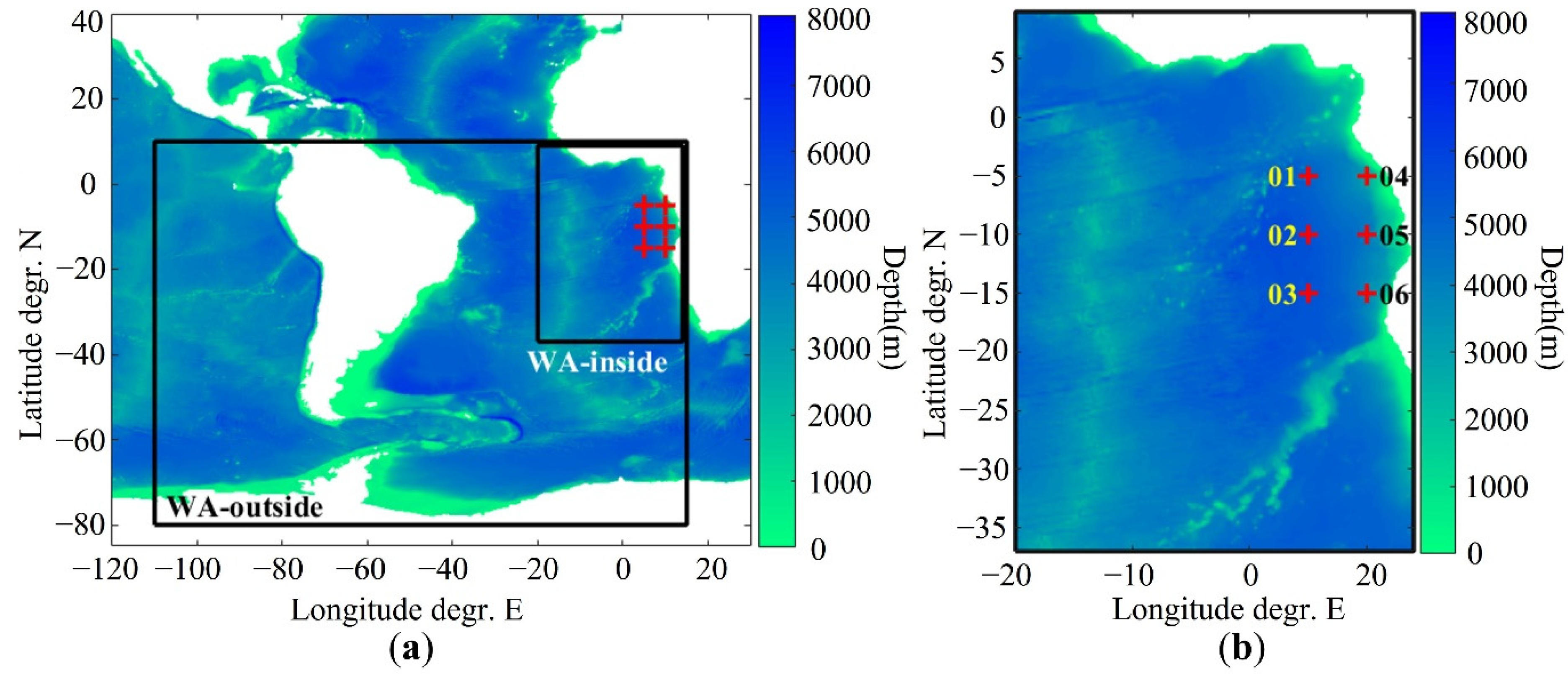
| SiteID | Latitude (°N) | Longitude (°N) | Depth (m) |
|---|---|---|---|
| P01 | −5 | 5 | 4949 |
| P02 | −10 | 5 | 5423 |
| P03 | −15 | 5 | 5488 |
| P04 | −5 | 10 | 2929 |
| P05 | −10 | 10 | 4294 |
| P06 | −15 | 10 | 3798 |
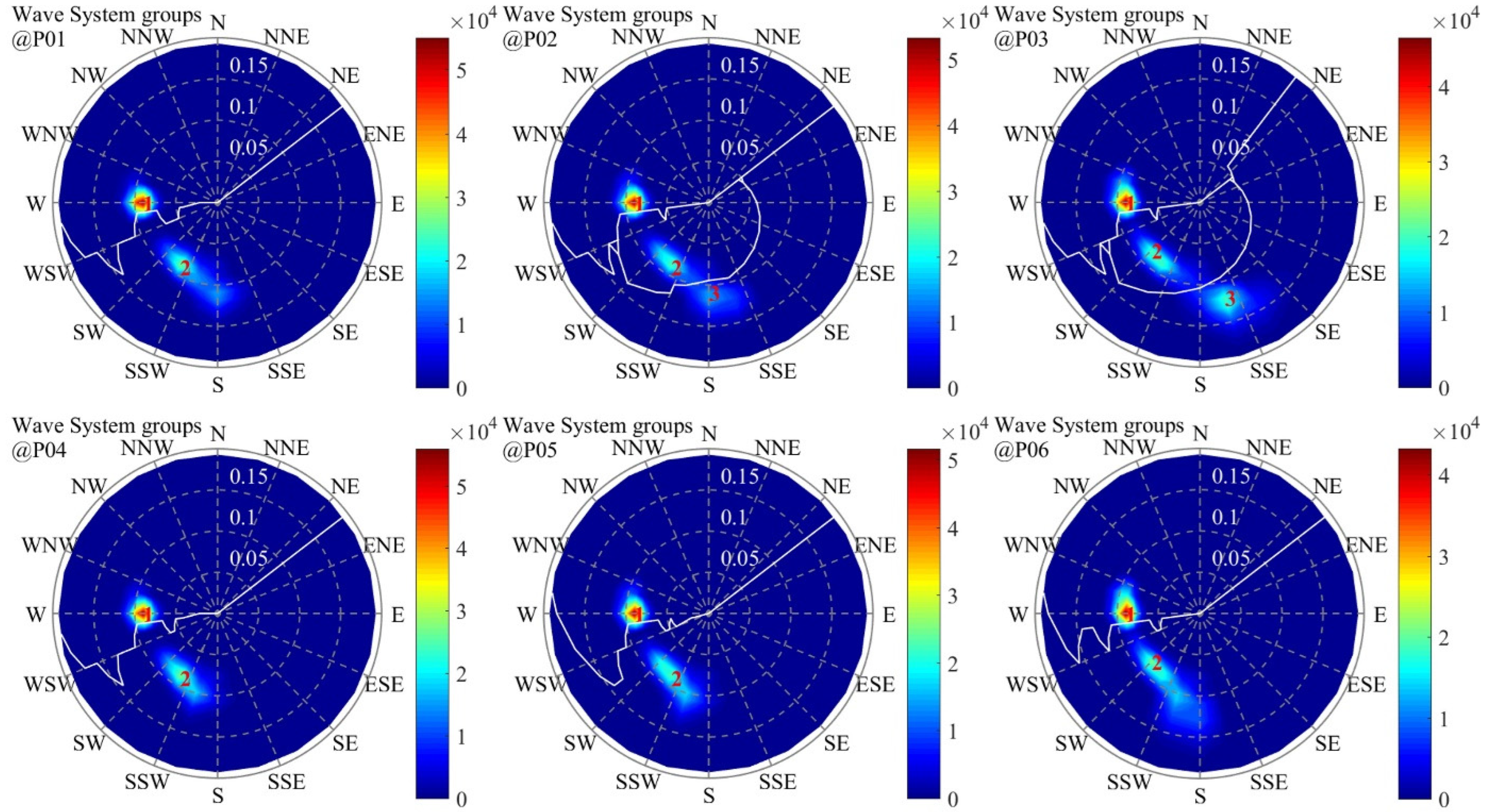
| SiteID | Accumulated J Contained in Each Group (Yearly Averaged, MW/m) | Number of Systems Occurring in Each Group (Yearly Averaged) | ||||
|---|---|---|---|---|---|---|
| grp-1 | grp-2 | grp-3 | grp-1 | grp-2 | grp-3 | |
| P01 | 25.32 | 96.95 | - | 9382.85 | 14,593.35 | - |
| P02 | 34.74 | 91.98 | 27.11 | 9188.55 | 10,459.90 | 4748.95 |
| P03 | 45.05 | 106.36 | 47.53 | 8743.70 | 10,557.35 | 6256.60 |
| P04 | 29.48 | 93.40 | - | 9437.35 | 13,300.50 | - |
| P05 | 38.36 | 113.40 | - | 9089.20 | 13,194.15 | - |
| P06 | 46.91 | 154.80 | - | 8543.30 | 13,927.95 | - |
Publisher’s Note: MDPI stays neutral with regard to jurisdictional claims in published maps and institutional affiliations. |
© 2022 by the authors. Licensee MDPI, Basel, Switzerland. This article is an open access article distributed under the terms and conditions of the Creative Commons Attribution (CC BY) license (https://creativecommons.org/licenses/by/4.0/).
Share and Cite
Jiang, X.; Gao, D.; Hua, F.; Yang, Y.; Wang, Z. An Improved Approach to Wave Energy Resource Characterization for Sea States with Multiple Wave Systems. J. Mar. Sci. Eng. 2022, 10, 1362. https://doi.org/10.3390/jmse10101362
Jiang X, Gao D, Hua F, Yang Y, Wang Z. An Improved Approach to Wave Energy Resource Characterization for Sea States with Multiple Wave Systems. Journal of Marine Science and Engineering. 2022; 10(10):1362. https://doi.org/10.3390/jmse10101362
Chicago/Turabian StyleJiang, Xingjie, Dalu Gao, Feng Hua, Yongzeng Yang, and Zeyu Wang. 2022. "An Improved Approach to Wave Energy Resource Characterization for Sea States with Multiple Wave Systems" Journal of Marine Science and Engineering 10, no. 10: 1362. https://doi.org/10.3390/jmse10101362