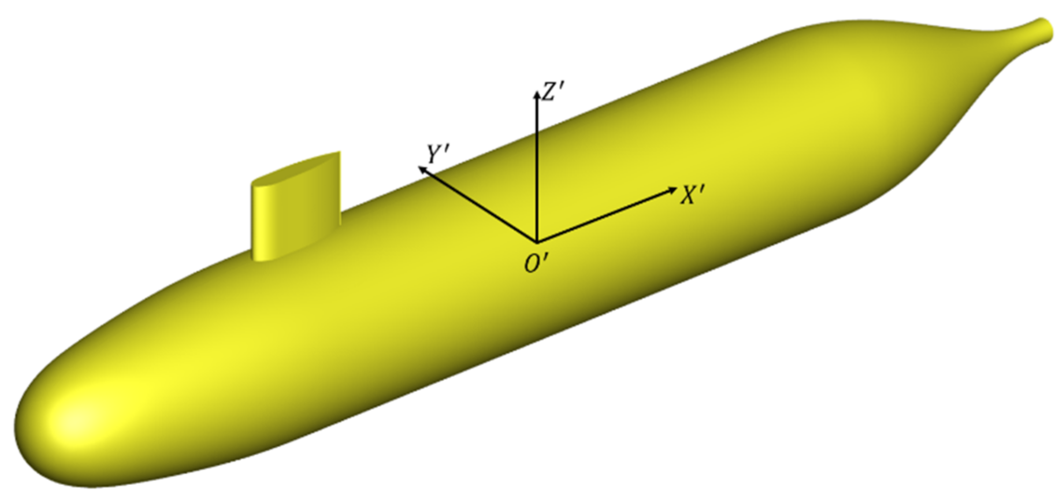
Figure 1.
Geometry of the SUBOFF model with the fairwater.
Figure 1.
Geometry of the SUBOFF model with the fairwater.
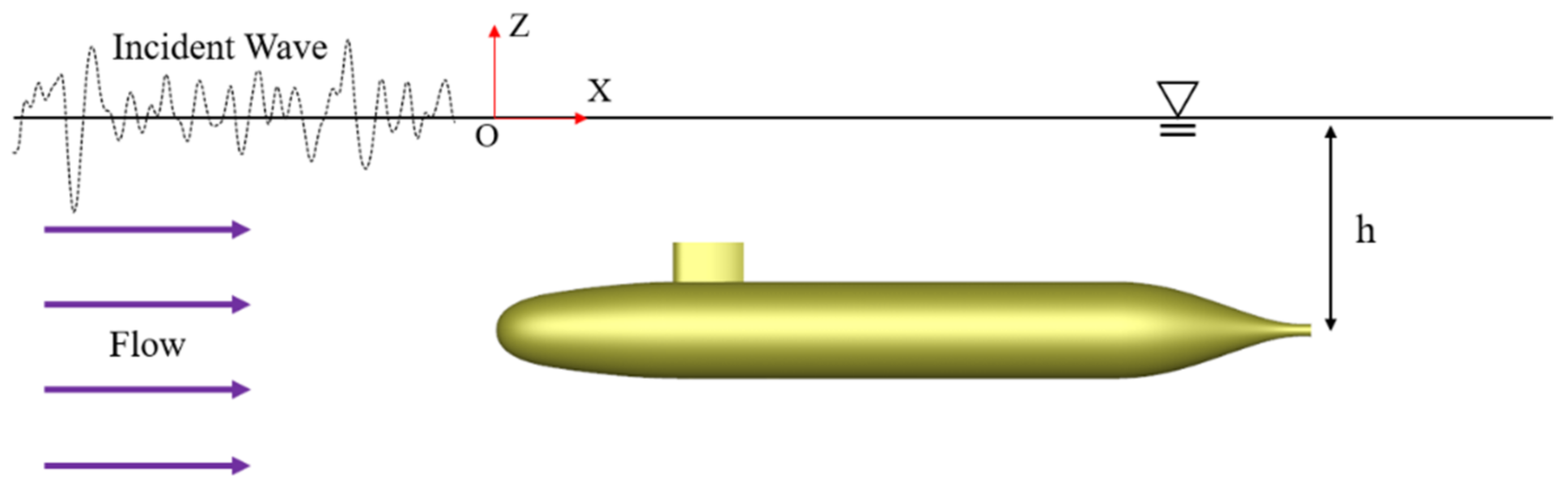
Figure 2.
General view of the simulation conditions.
Figure 2.
General view of the simulation conditions.
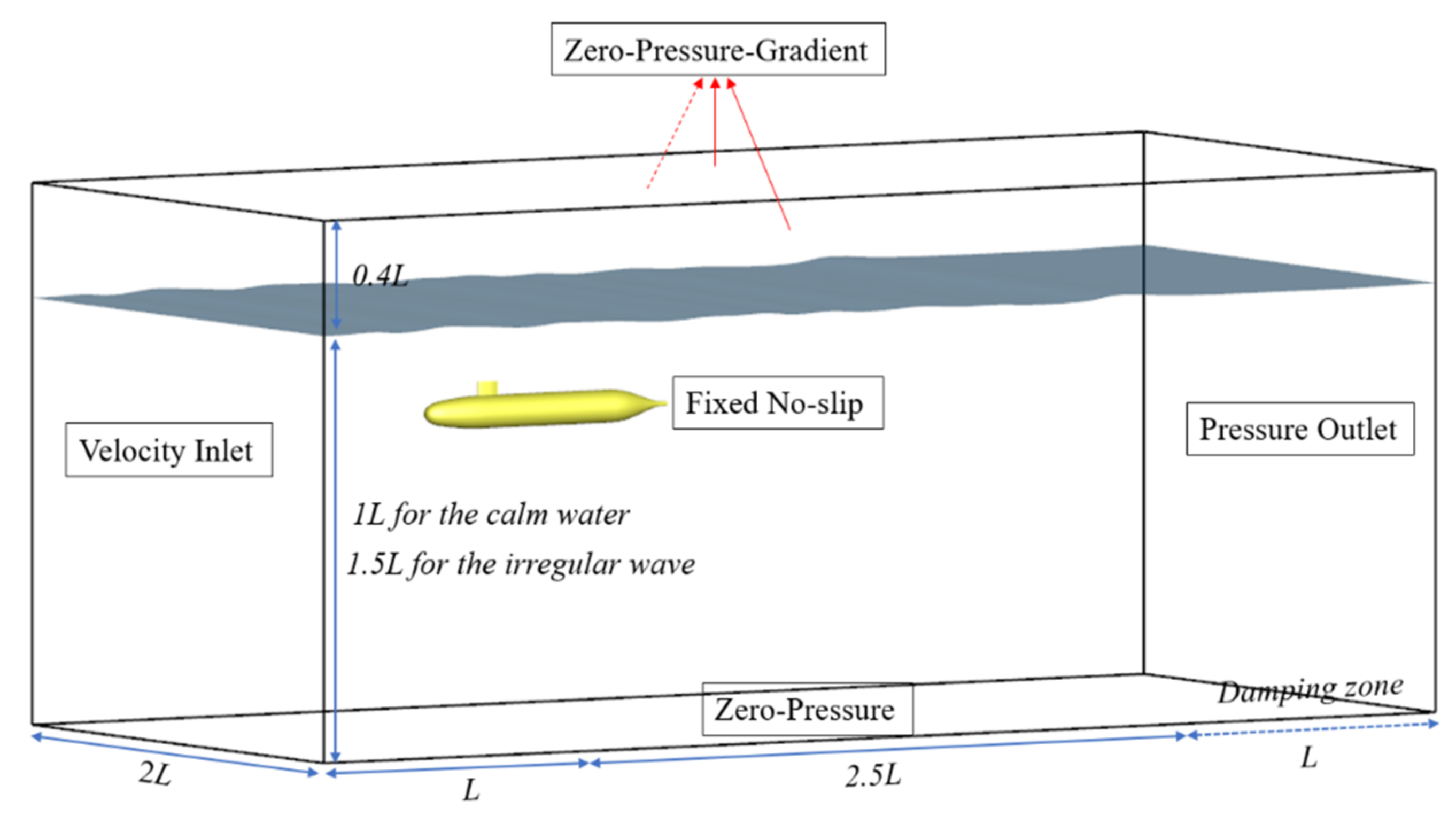
Figure 3.
Computational domain and boundary conditions of the model.
Figure 3.
Computational domain and boundary conditions of the model.
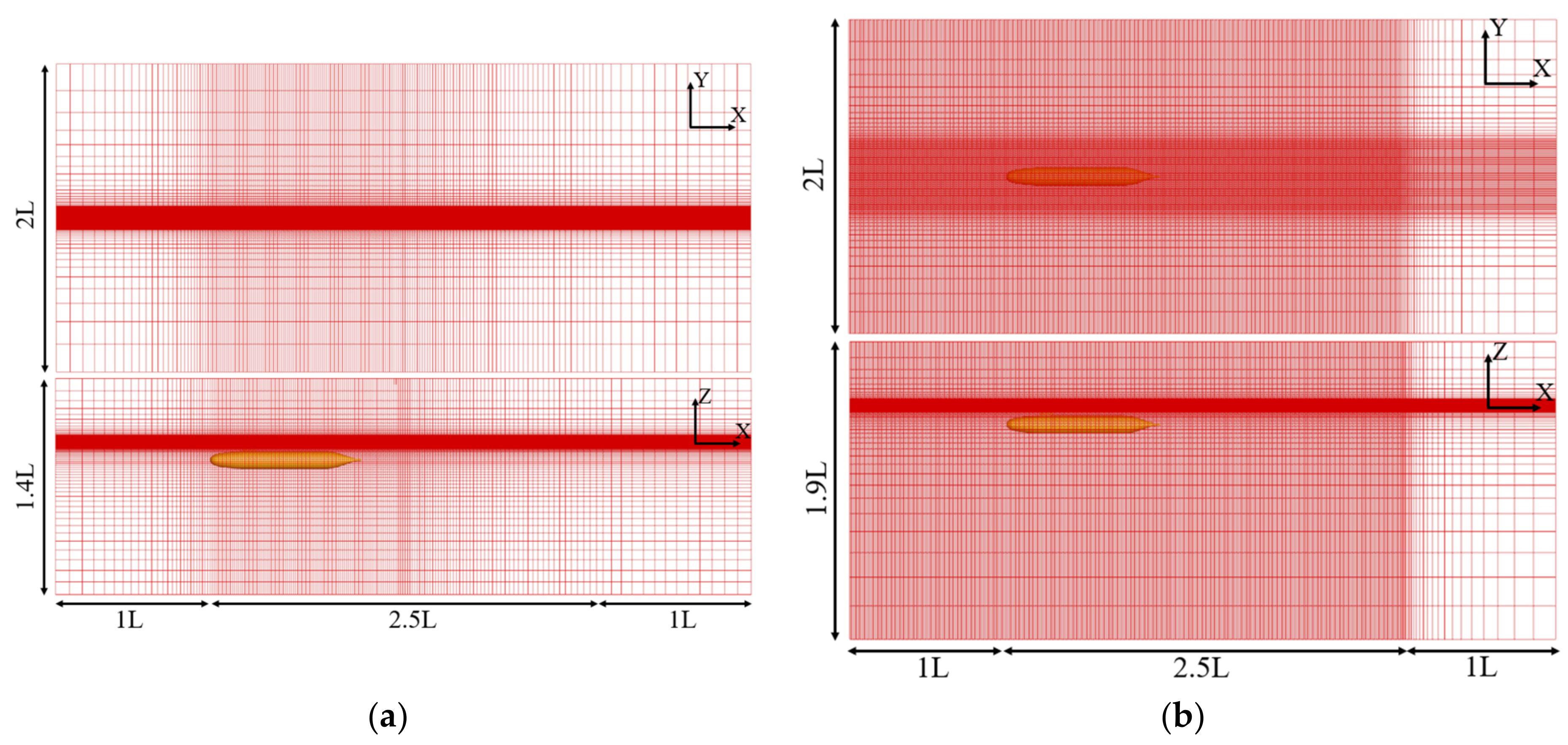
Figure 4.
Background grids for calm water and irregular waves conditions: (a) calm water; (b) irregular waves.
Figure 4.
Background grids for calm water and irregular waves conditions: (a) calm water; (b) irregular waves.
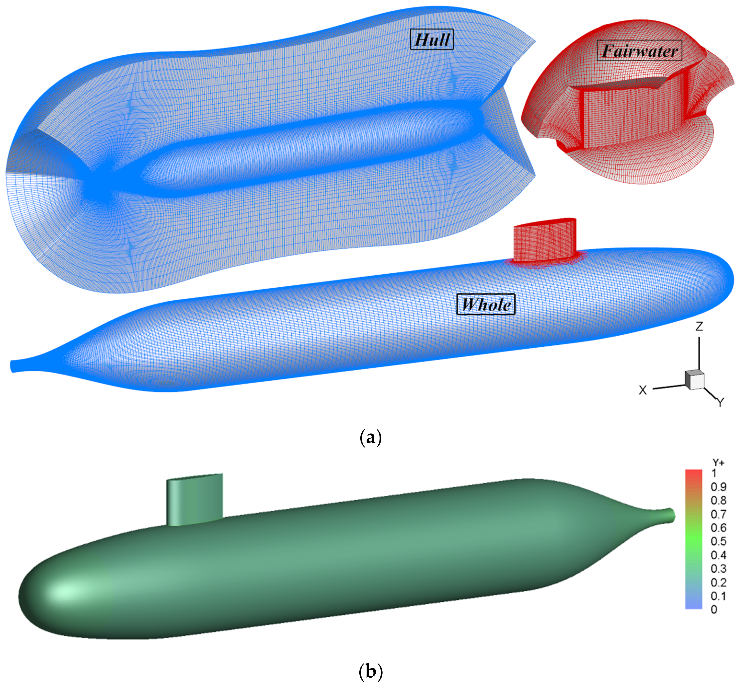
Figure 5.
The hull grids and appendage grids and the wall Y+ on the model surface: (a) hull and appendage grids; (b) Y+ on the model surface.
Figure 5.
The hull grids and appendage grids and the wall Y+ on the model surface: (a) hull and appendage grids; (b) Y+ on the model surface.
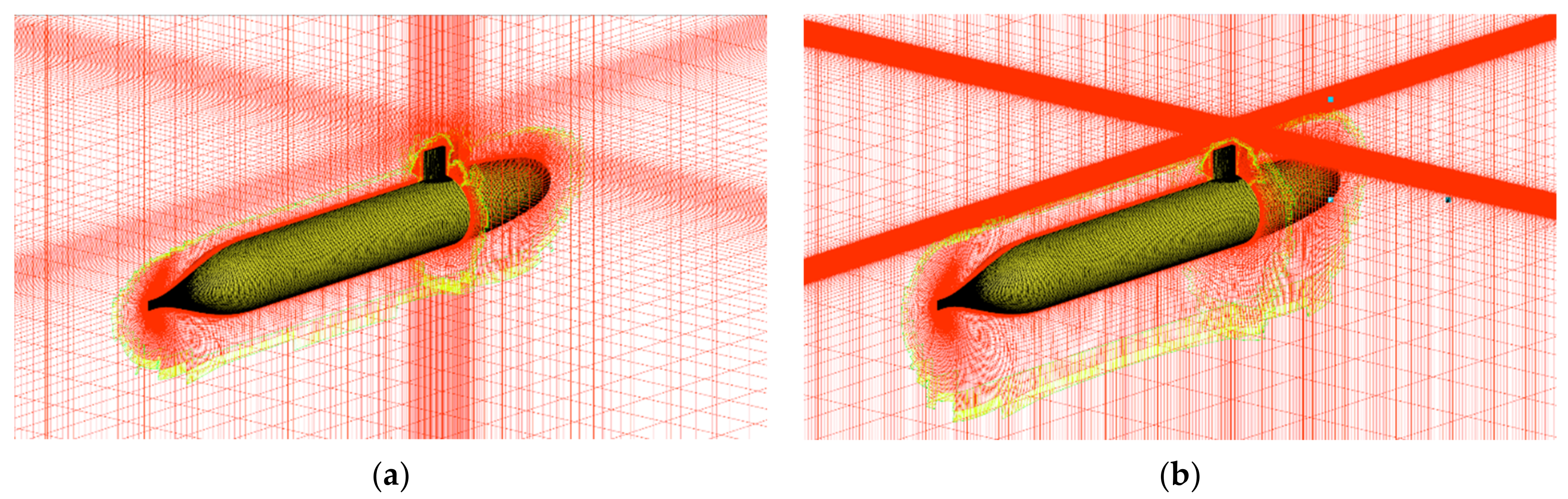
Figure 6.
Grid around the model after overset for calm water and irregular waves conditions: (a) calm water; (b) irregular waves.
Figure 6.
Grid around the model after overset for calm water and irregular waves conditions: (a) calm water; (b) irregular waves.
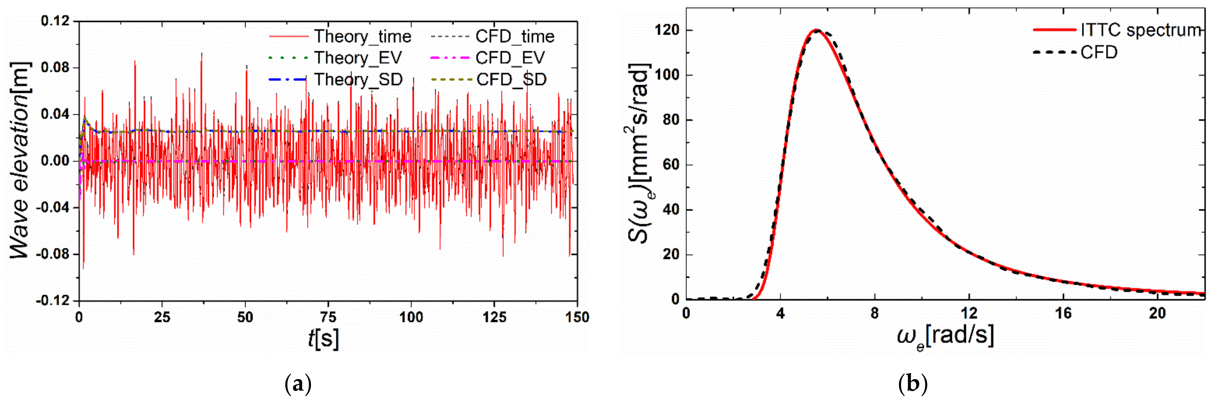
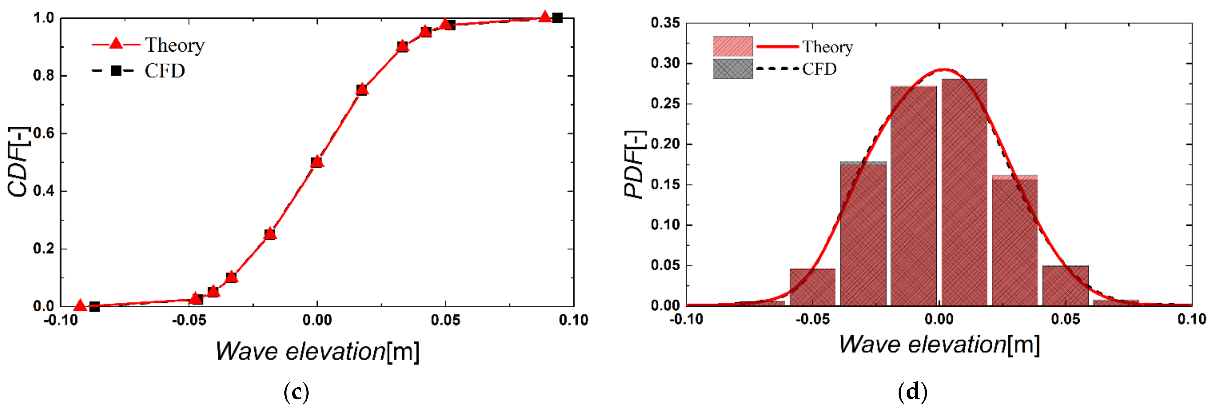
Figure 7.
Comparison between the CFD results and the theoretical values for the generation of long-crested waves: (a) time histories; (b) wave spectrum; (c) CDF; (d) PDF.
Figure 7.
Comparison between the CFD results and the theoretical values for the generation of long-crested waves: (a) time histories; (b) wave spectrum; (c) CDF; (d) PDF.
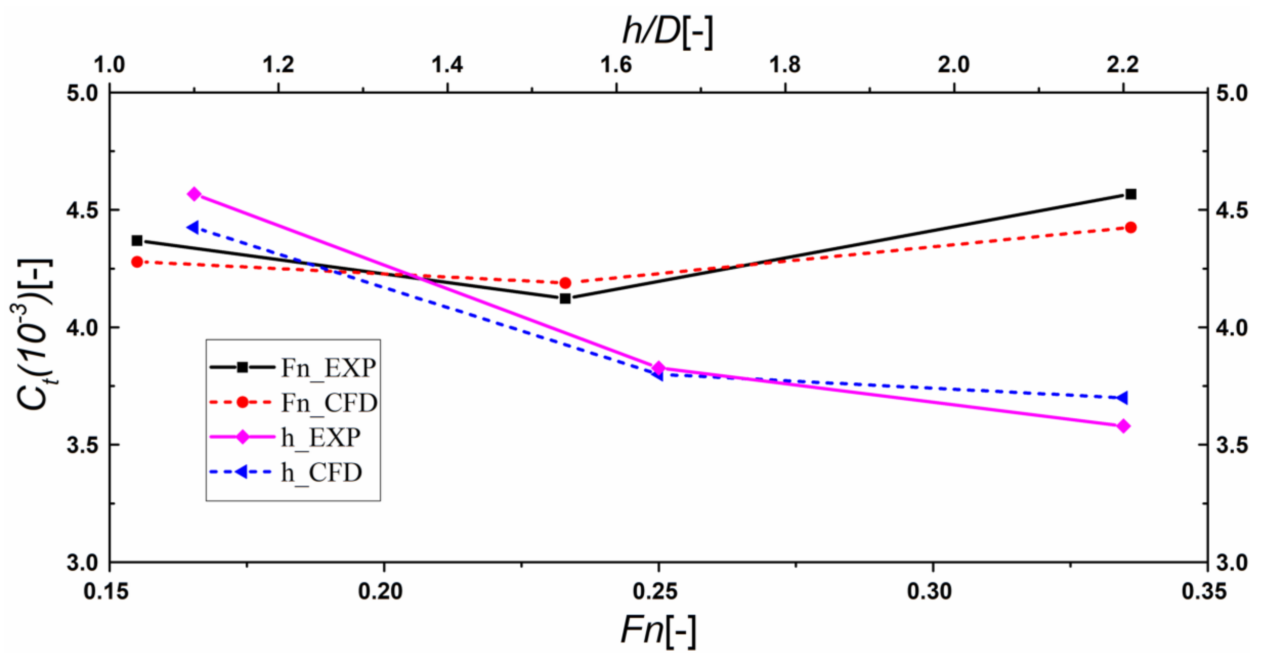
Figure 8.
Comparison between CFD and EFD for the total resistance coefficient of a submarine sailing near calm water with different velocities and submerged depths.
Figure 8.
Comparison between CFD and EFD for the total resistance coefficient of a submarine sailing near calm water with different velocities and submerged depths.
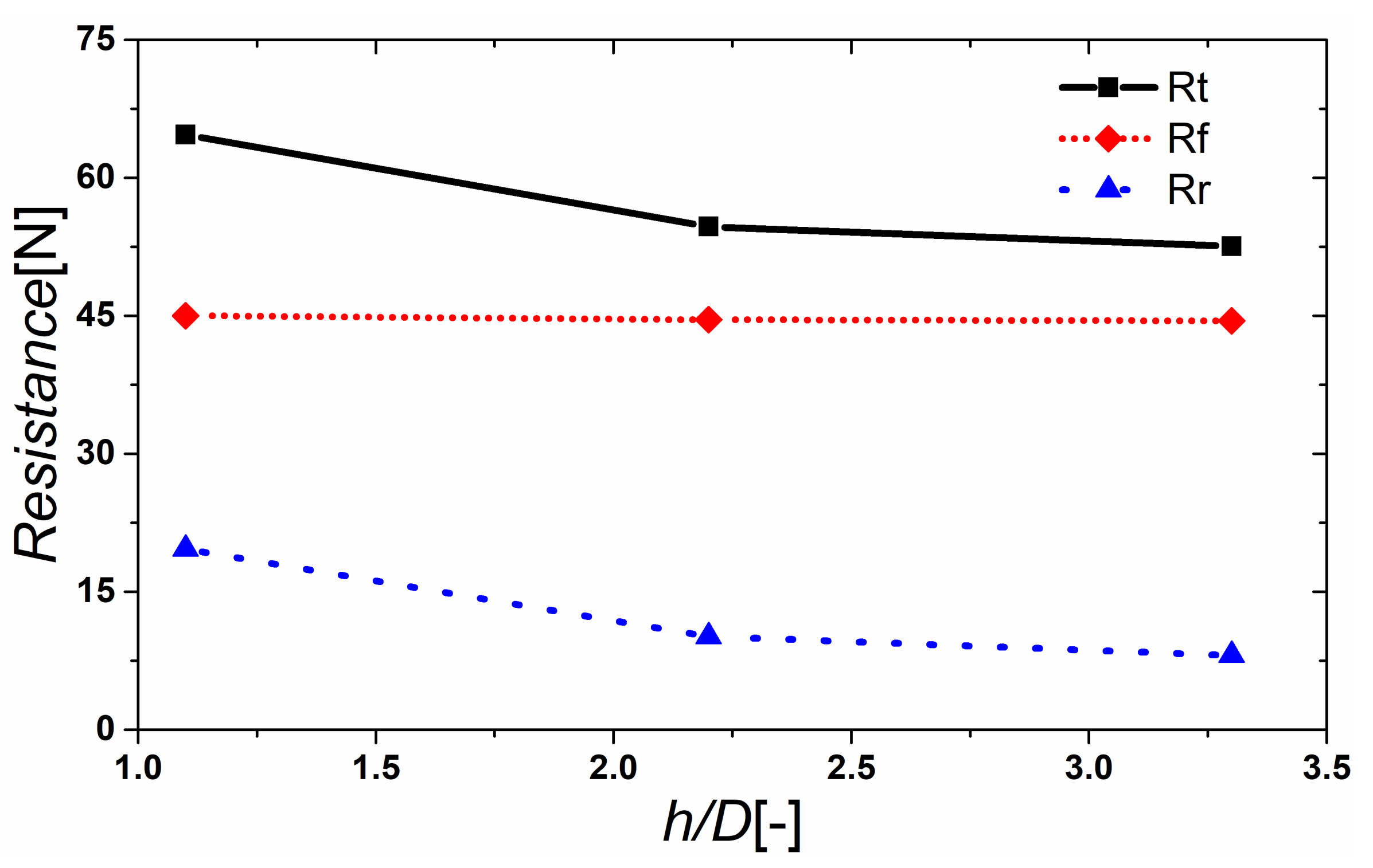
Figure 9.
The resistance of the model sailing near the free surface in calm water at different submerged depths.
Figure 9.
The resistance of the model sailing near the free surface in calm water at different submerged depths.
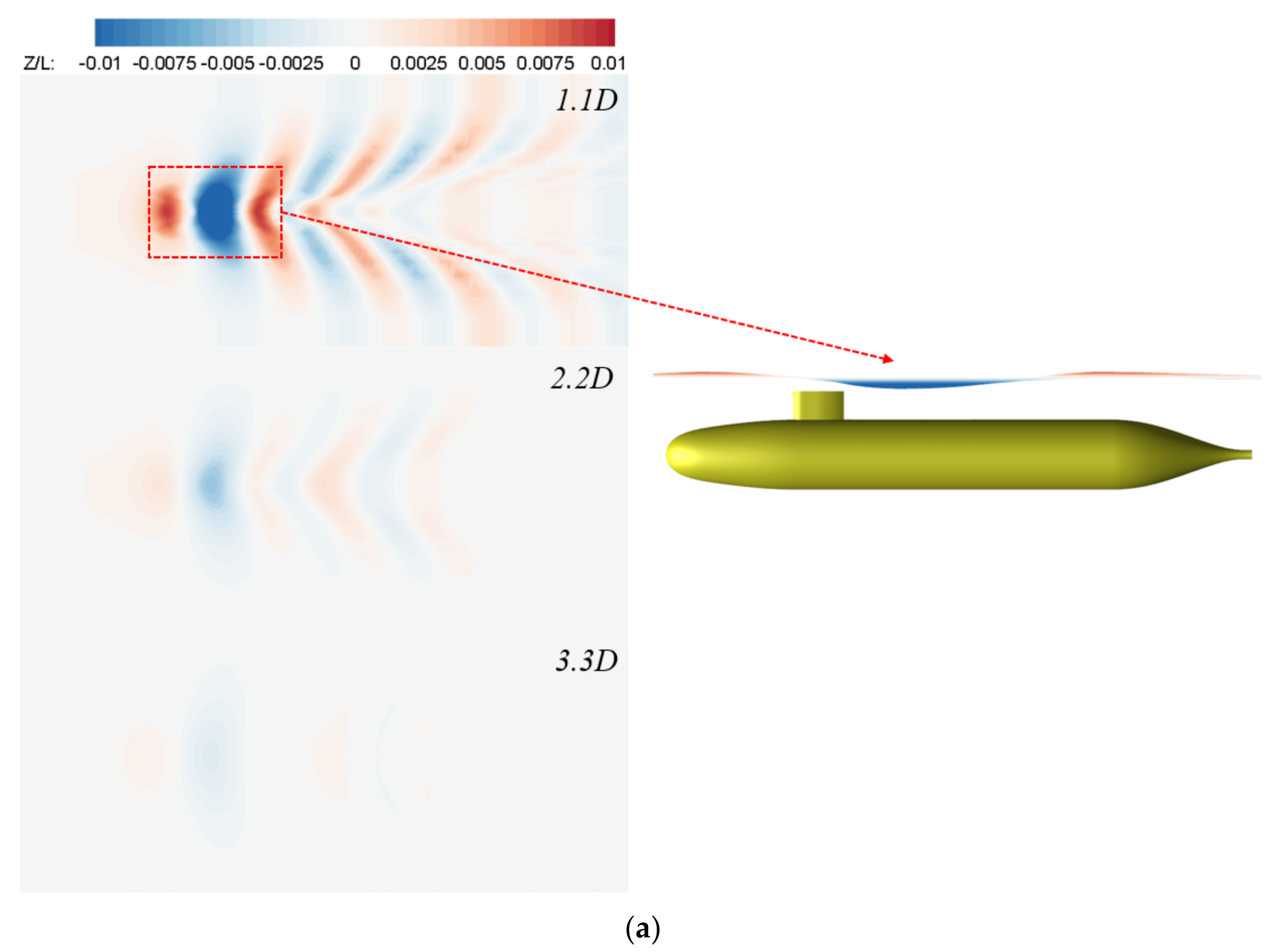
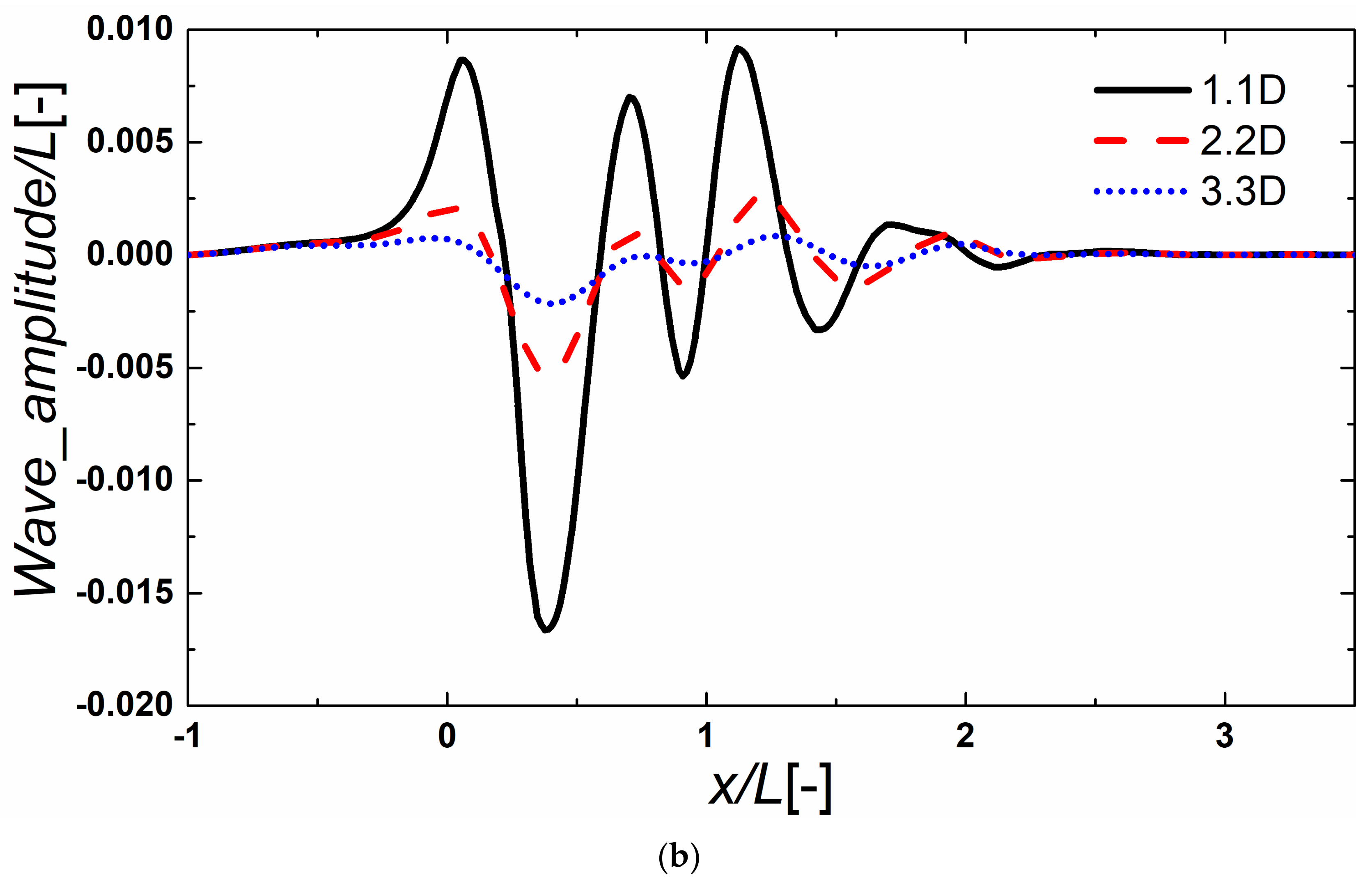
Figure 10.
The free surface at different submerged depths: (a) wave pattern; (b) wave amplitude.
Figure 10.
The free surface at different submerged depths: (a) wave pattern; (b) wave amplitude.
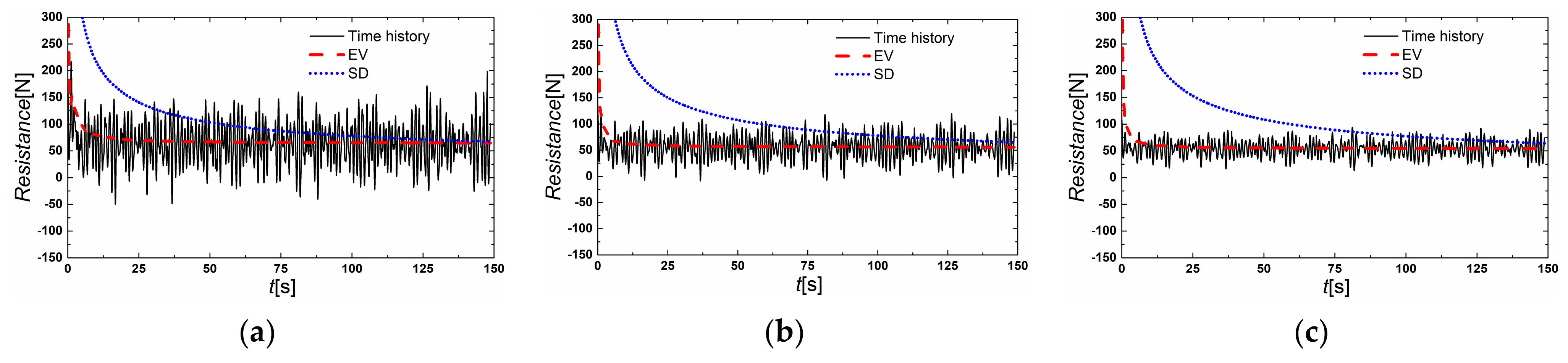
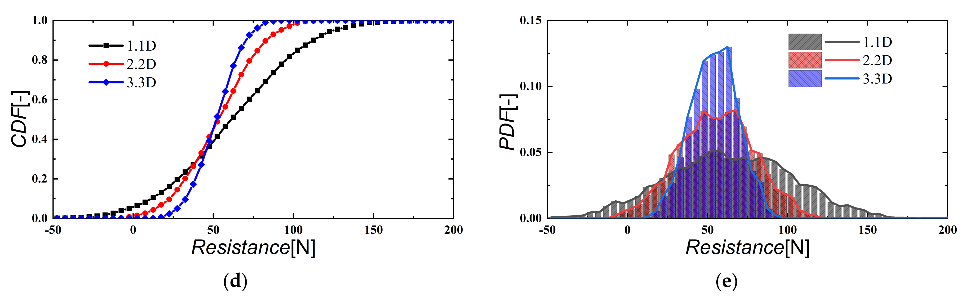
Figure 11.
The resistance of the model sailing near the free surface with irregular waves at different submerged depths: (a) 1.1D; (b) 2.2D; (c) 3.3D; (d) CDF; (e) PDF.
Figure 11.
The resistance of the model sailing near the free surface with irregular waves at different submerged depths: (a) 1.1D; (b) 2.2D; (c) 3.3D; (d) CDF; (e) PDF.
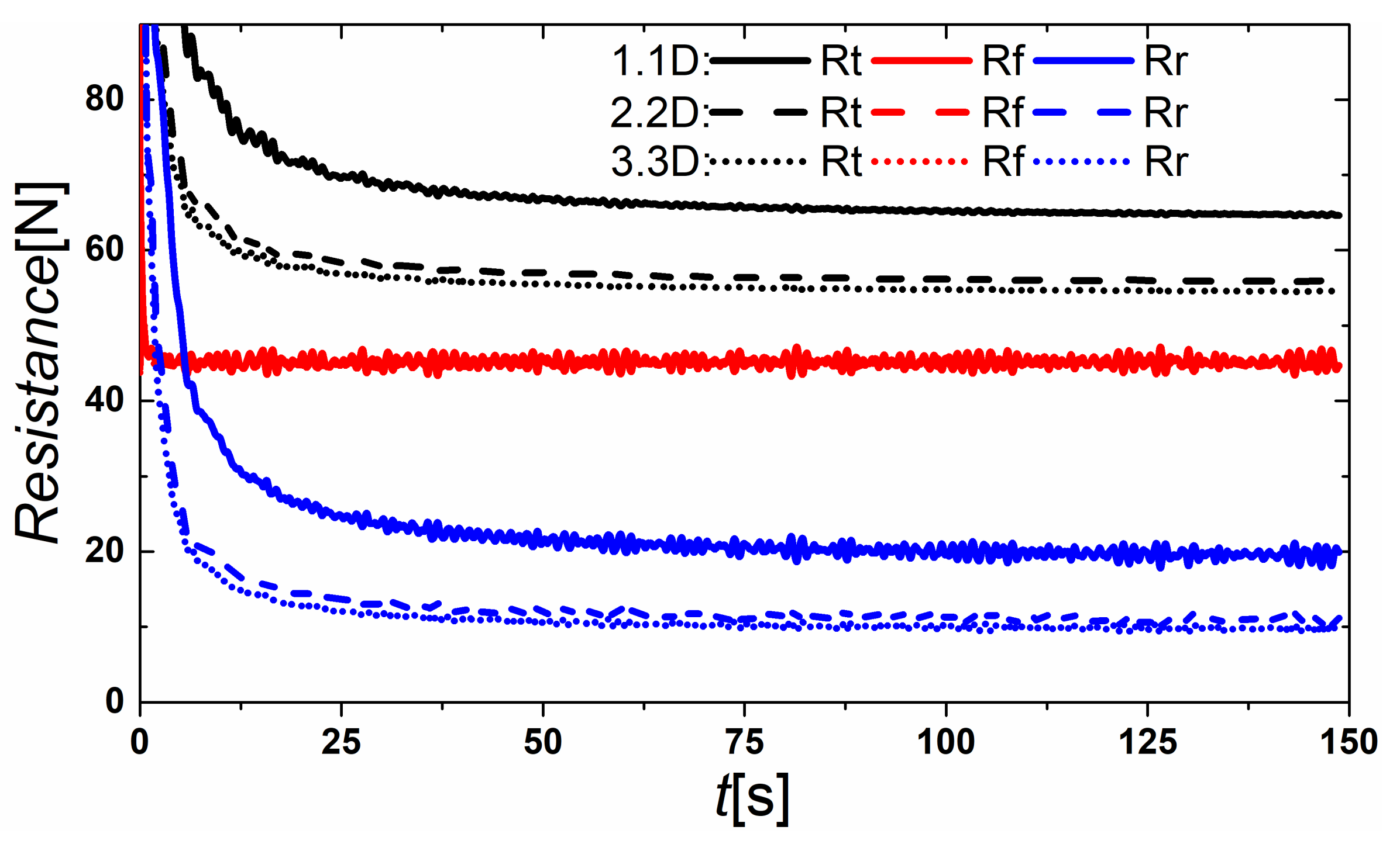
Figure 12.
The EV of different resistance components for the model sailing near the free surface with irregular waves at different submerged depths.
Figure 12.
The EV of different resistance components for the model sailing near the free surface with irregular waves at different submerged depths.
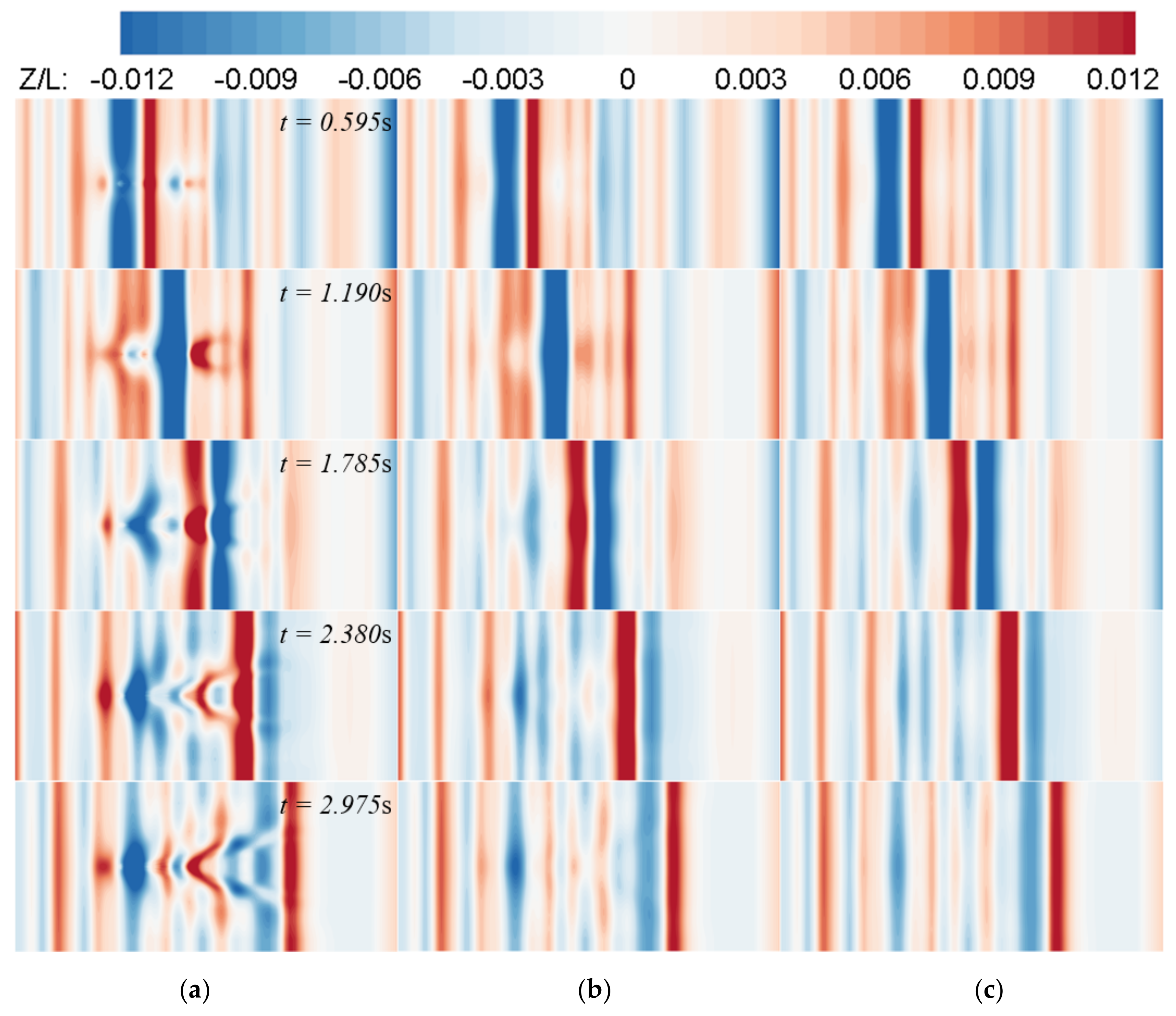
Figure 13.
The snapshot of the wave pattern in the very beginning of the solution times: (a) 1.1D; (b) 2.2D; (c) 3.3D.
Figure 13.
The snapshot of the wave pattern in the very beginning of the solution times: (a) 1.1D; (b) 2.2D; (c) 3.3D.
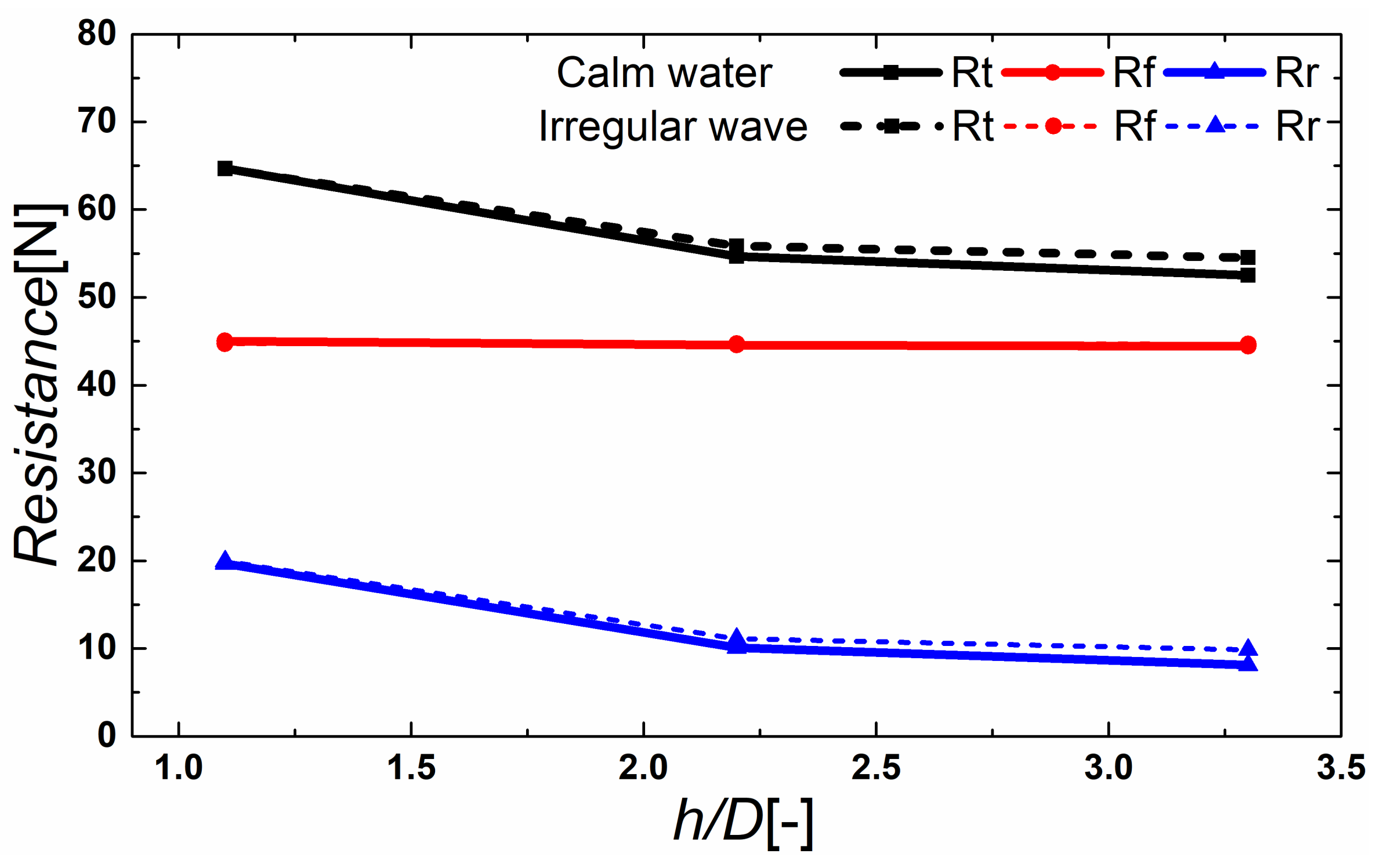
Figure 14.
The comparison of the total resistance between calm water and the EV of irregular wave conditions at different submerged depths.
Figure 14.
The comparison of the total resistance between calm water and the EV of irregular wave conditions at different submerged depths.
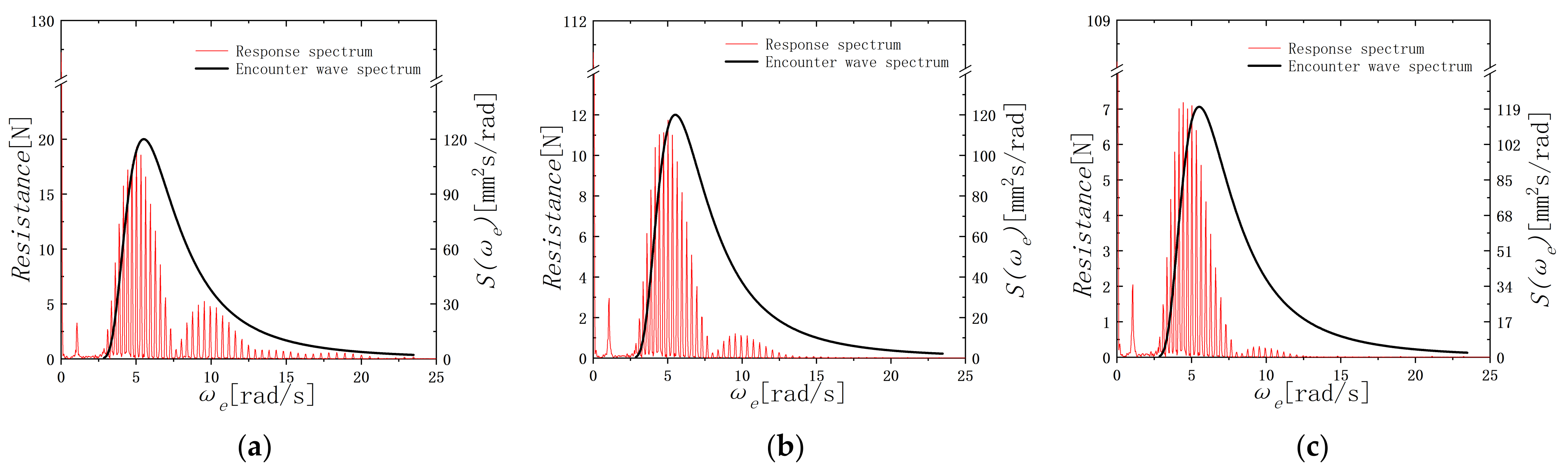
Figure 15.
The spectral response of resistance for the model sailing near the free surface with irregular waves at different submerged depths: (a) 1.1D; (b) 2.2D; (c) 3.3D.
Figure 15.
The spectral response of resistance for the model sailing near the free surface with irregular waves at different submerged depths: (a) 1.1D; (b) 2.2D; (c) 3.3D.
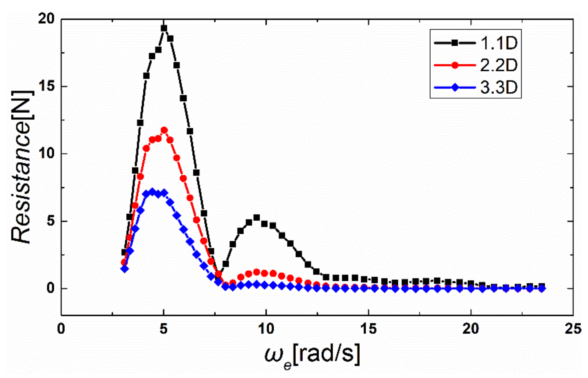
Figure 16.
The comparison of the total resistance spectral response at different submerged depths.
Figure 16.
The comparison of the total resistance spectral response at different submerged depths.
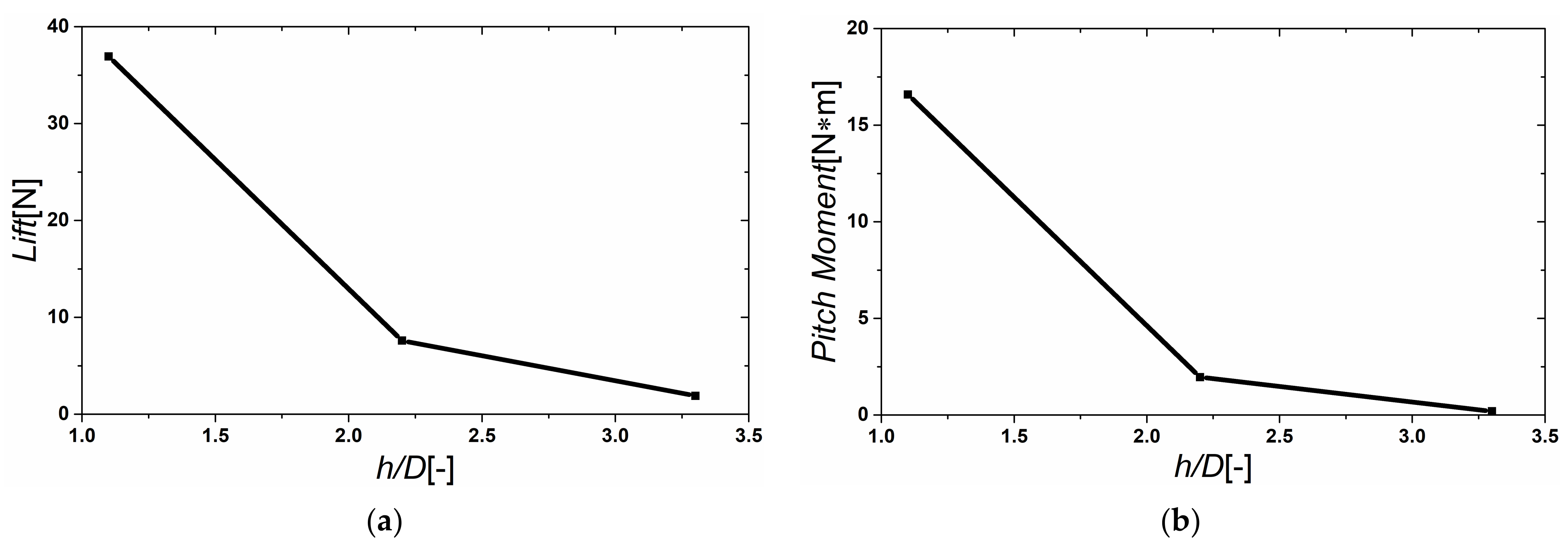
Figure 17.
The lift and pitch moments of the model sailing near the free surface in calm water at different submerged depths: (a) lift; (b) pitch moment.
Figure 17.
The lift and pitch moments of the model sailing near the free surface in calm water at different submerged depths: (a) lift; (b) pitch moment.
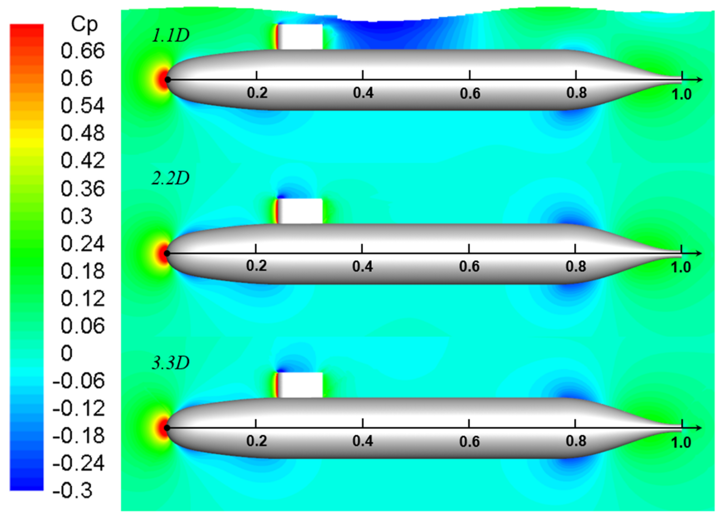
Figure 18.
The dynamic pressure distribution around the model on the XOZ plane at different submerged depths.
Figure 18.
The dynamic pressure distribution around the model on the XOZ plane at different submerged depths.
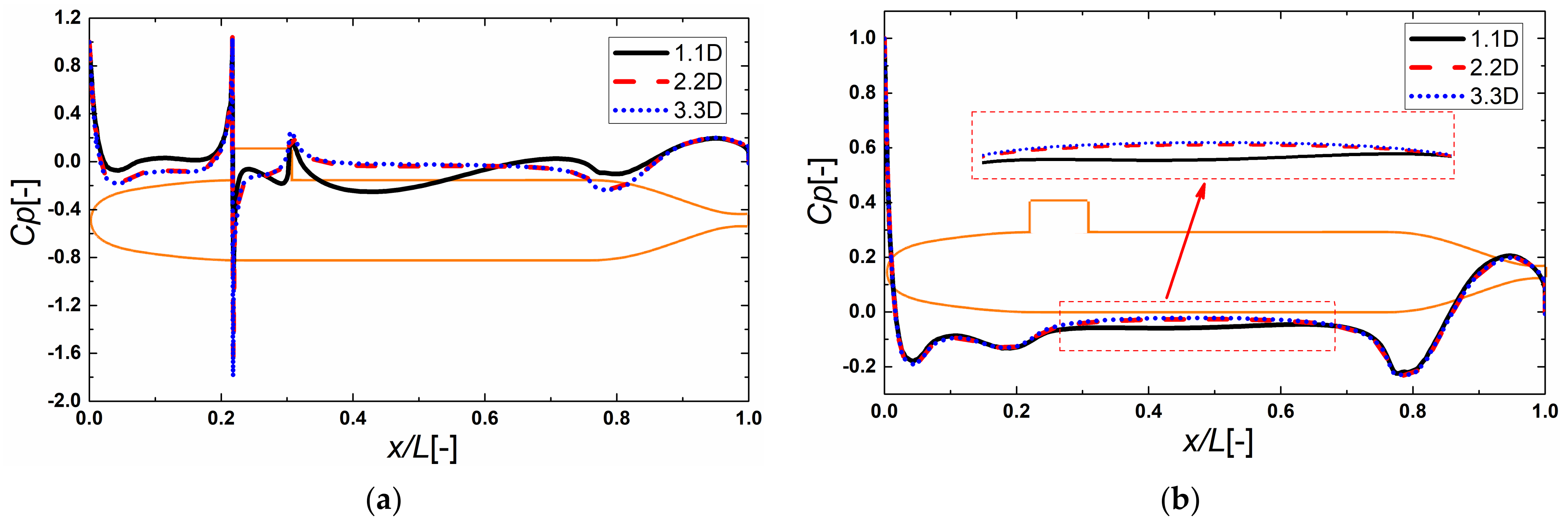
Figure 19.
The dynamic pressure distribution along the hull length at different submerged depths: (a) upper surface; (b) lower surface.
Figure 19.
The dynamic pressure distribution along the hull length at different submerged depths: (a) upper surface; (b) lower surface.
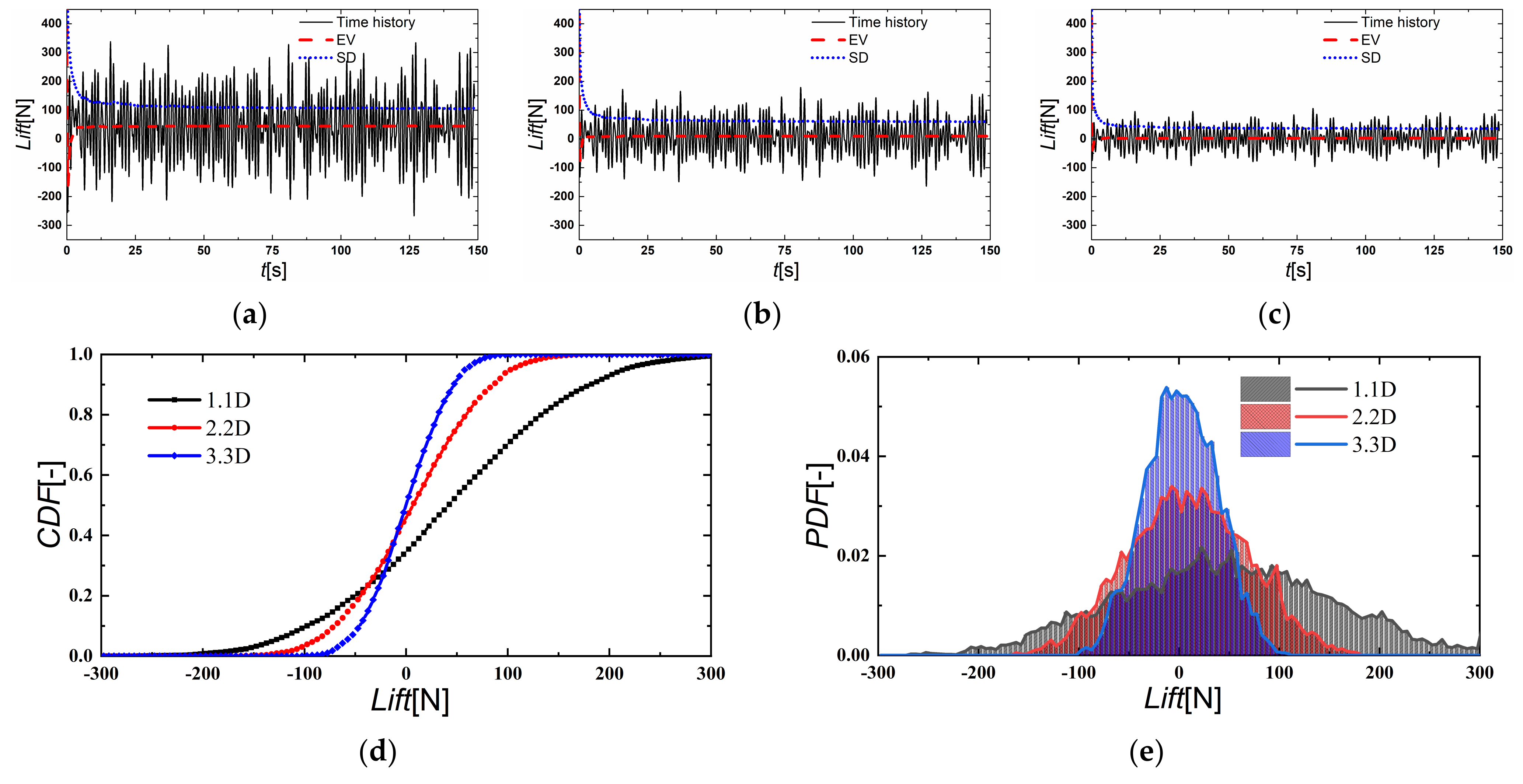
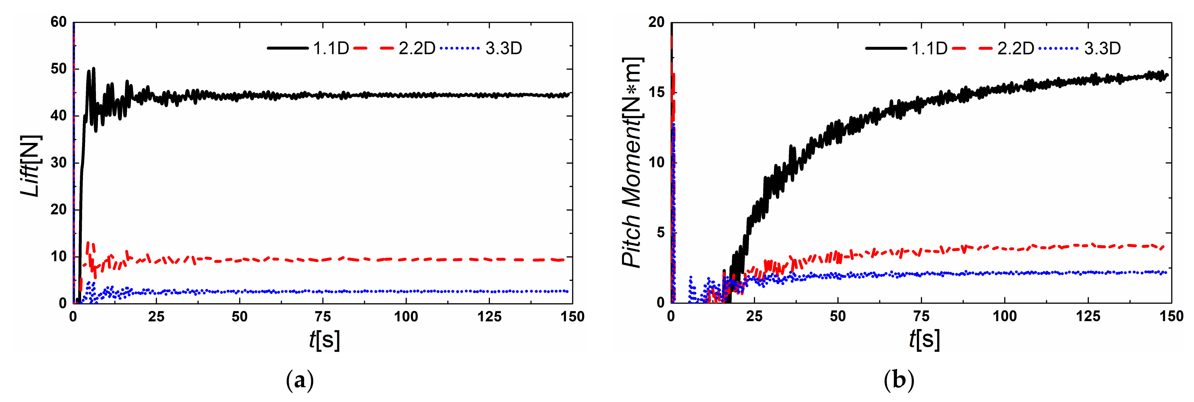
Figure 20.
The lift of the model sailing near the free surface with irregular waves at different submerged depths: (a) 1.1D; (b) 2.2D; (c) 3.3D; (d) CDF; (e) PDF.
Figure 20.
The lift of the model sailing near the free surface with irregular waves at different submerged depths: (a) 1.1D; (b) 2.2D; (c) 3.3D; (d) CDF; (e) PDF.
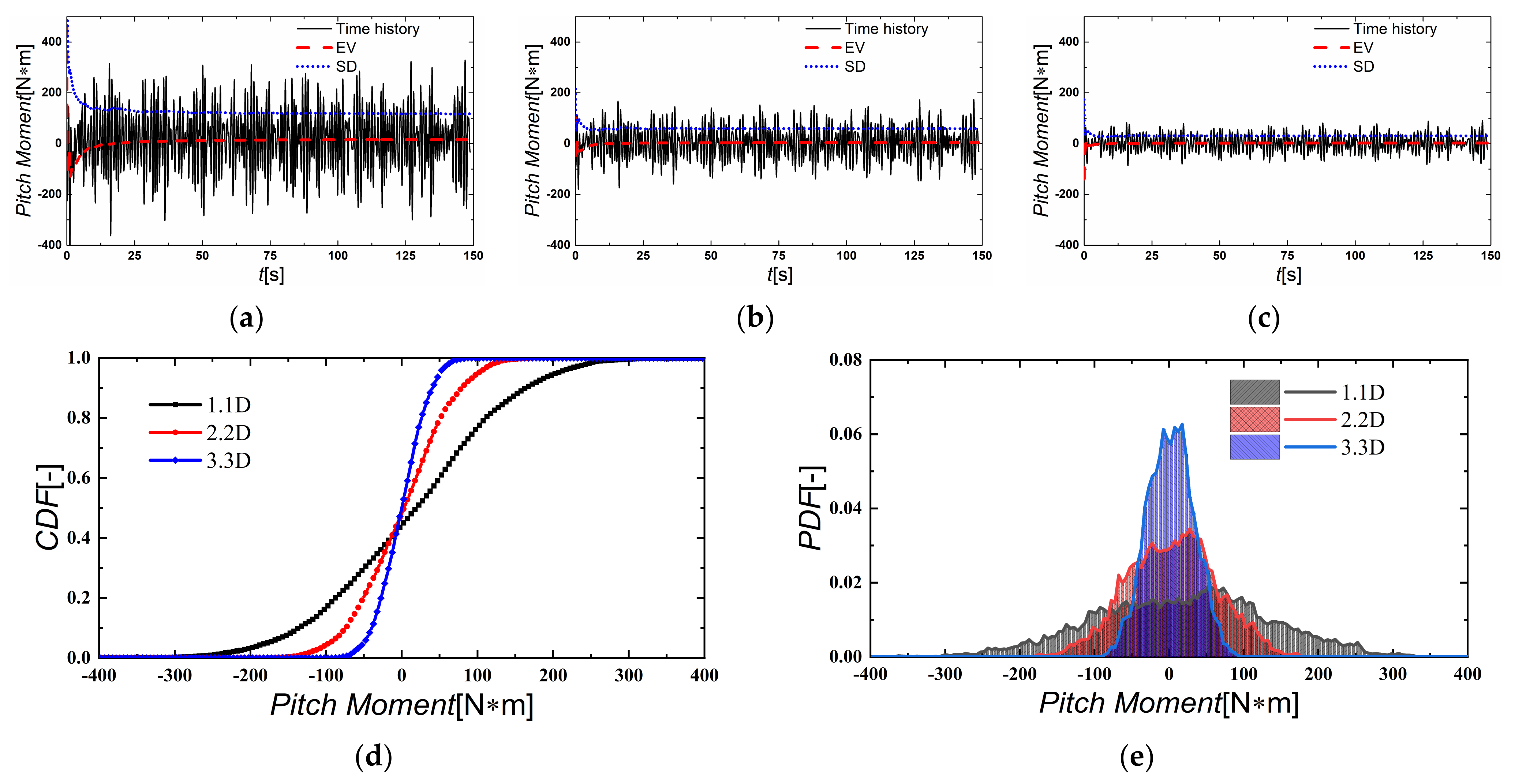
Figure 21.
The pitch moment of the model sailing near the free surface with irregular waves at different submerged depths: (a) 1.1D; (b) 2.2D; (c) 3.3D; (d) CDF; (e) PDF.
Figure 21.
The pitch moment of the model sailing near the free surface with irregular waves at different submerged depths: (a) 1.1D; (b) 2.2D; (c) 3.3D; (d) CDF; (e) PDF.
Figure 22.
The EV of the lift and pitch moments of the model sailing near the free surface with irregular waves at different submerged depths: (a) lift; (b) pitch moment.
Figure 22.
The EV of the lift and pitch moments of the model sailing near the free surface with irregular waves at different submerged depths: (a) lift; (b) pitch moment.
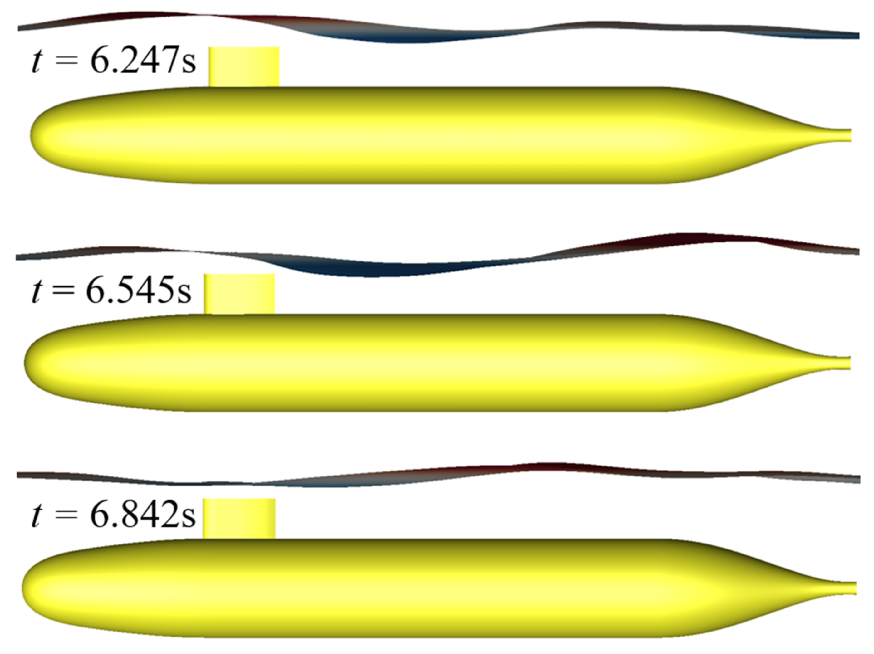
Figure 23.
The free surface at different solution times.
Figure 23.
The free surface at different solution times.
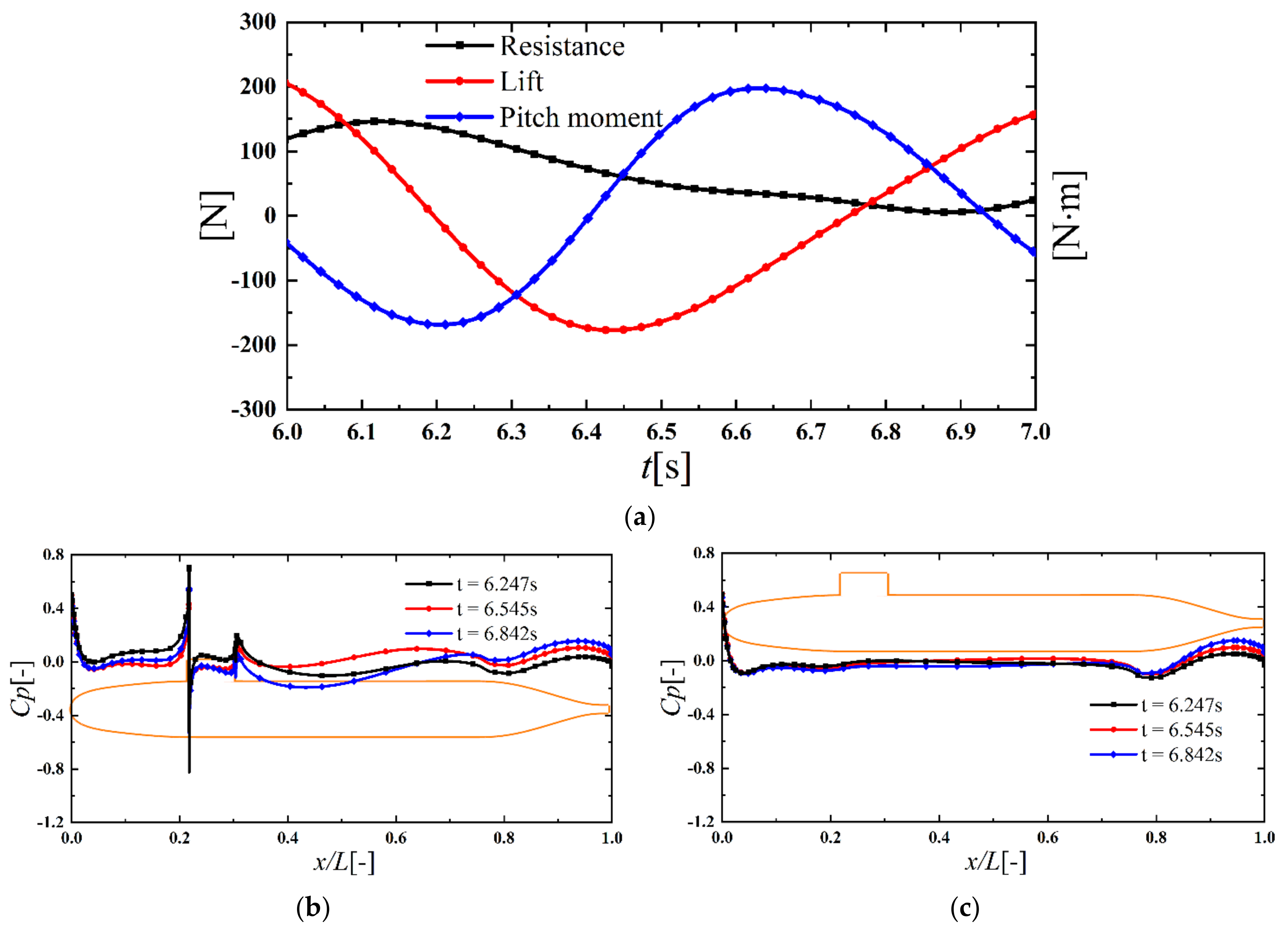
Figure 24.
The hydrodynamic forces, moments, and dynamic pressure distribution along the hull length at different solution times: (a) hydrodynamic force and moments; (b) upper surface; (c) lower surface.
Figure 24.
The hydrodynamic forces, moments, and dynamic pressure distribution along the hull length at different solution times: (a) hydrodynamic force and moments; (b) upper surface; (c) lower surface.
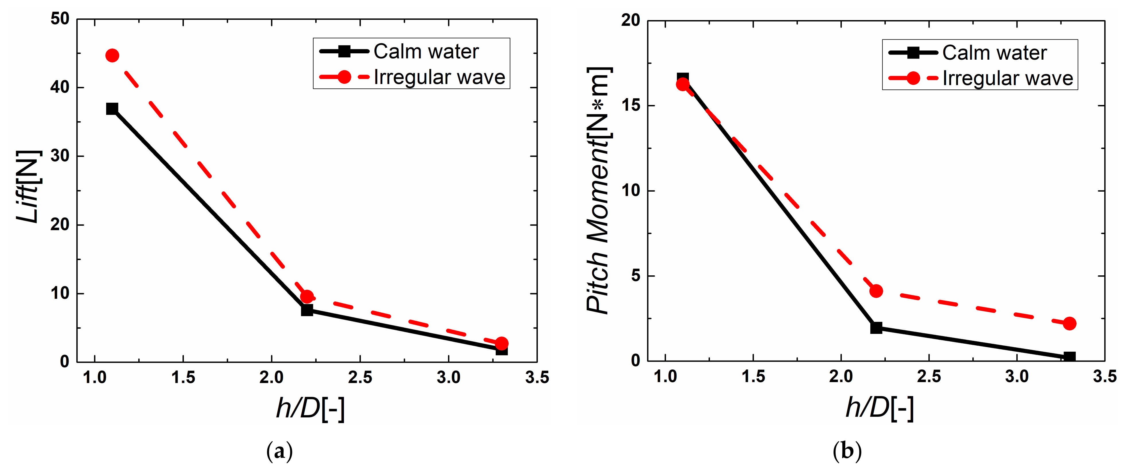
Figure 25.
The comparison of the lift and pitch moments between calm water and the EV of irregular wave conditions at different submerged depths: (a) lift; (b) pitch moment.
Figure 25.
The comparison of the lift and pitch moments between calm water and the EV of irregular wave conditions at different submerged depths: (a) lift; (b) pitch moment.
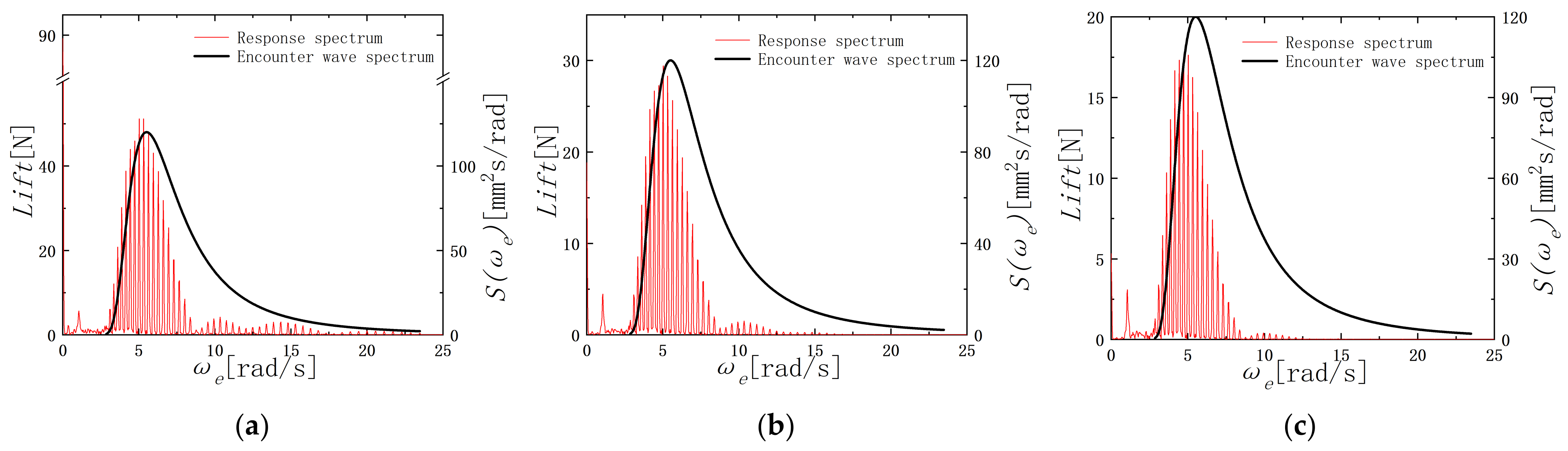
Figure 26.
The spectral response of the lift of the model sailing near the free surface with irregular waves at different submerged depths: (a) 1.1D; (b) 2.2D; (c) 3.3D.
Figure 26.
The spectral response of the lift of the model sailing near the free surface with irregular waves at different submerged depths: (a) 1.1D; (b) 2.2D; (c) 3.3D.
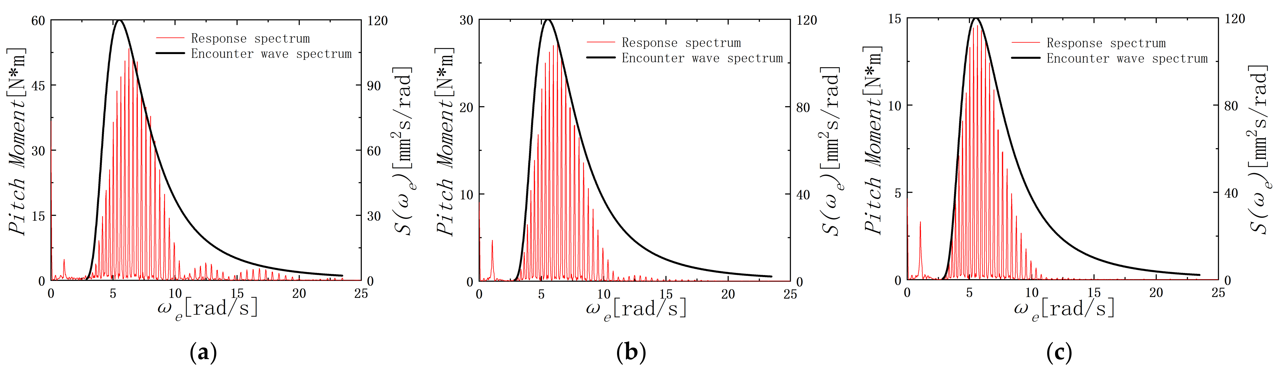
Figure 27.
The spectral response of the pitch moment of the model sailing near the free surface with irregular waves at different submerged depths: (a) 1.1D; (b) 2.2D; (c) 3.3D.
Figure 27.
The spectral response of the pitch moment of the model sailing near the free surface with irregular waves at different submerged depths: (a) 1.1D; (b) 2.2D; (c) 3.3D.
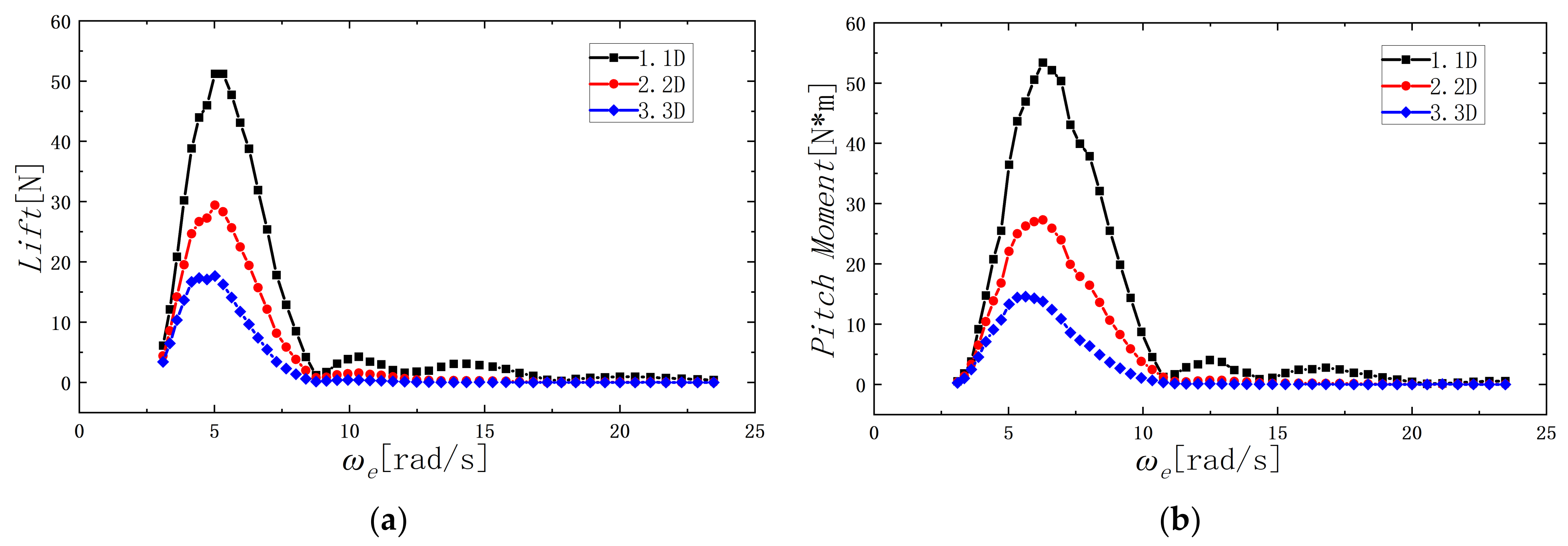
Figure 28.
The comparison of the spectral response for the lift and pitch moments at different submerged depths: (a) lift; (b) pitch moment.
Figure 28.
The comparison of the spectral response for the lift and pitch moments at different submerged depths: (a) lift; (b) pitch moment.
Table 1.
Main parameters of the SUBOFF model.
Table 1.
Main parameters of the SUBOFF model.
| Parameters | Symbol | Units | Model |
|---|
| Hull length | L | m | 4.356 |
| Hull diameter | D | m | 0.508 |
| Center of gravity | Xg | m | 1.975 |
| Wetted-surface area | S | m2 | 6.058 |
Table 2.
Description of the simulation conditions.
Table 2.
Description of the simulation conditions.
| Case | Froude Number | Depths (h/D) | Sea State | Free Surface |
|---|
| 1 | 0.336 | 1.1 | - | Calm water |
| 2 | 0.336 | 2.2 | - | Calm water |
| 3 | 0.336 | 3.3 | - | Calm water |
| 4 | 0.336 | 1.1 | 4 | Irregular waves |
| 5 | 0.336 | 2.2 | 4 | Irregular waves |
| 6 | 0.336 | 3.3 | 4 | Irregular waves |
Table 3.
The 0th order moment, m0, of the spectrum, ωe, and S(ωe) corresponding to the peak point of the spectrum.
Table 3.
The 0th order moment, m0, of the spectrum, ωe, and S(ωe) corresponding to the peak point of the spectrum.
| | ωe | S(ωe) | m0 |
|---|
| CFD | 5.747 | 119.996 | 664.72 |
| Theory | 5.516 | 119.992 | 657.72 |
| Diff. (%) | 4.2% | <0.1% | 1.1% |
Table 4.
Details for different grid nodes.
Table 4.
Details for different grid nodes.
| Grid Nodes (M *) | Hull | Fairwater | Background | Total |
|---|
| Coarse | 1.37 | 0.18 | 0.41 | 1.96 |
| Medium | 3.87 | 0.50 | 1.18 | 5.55 |
| Fine | 11.07 | 1.44 | 3.46 | 15.97 |
Table 5.
Verification study for the total resistance.
Table 5.
Verification study for the total resistance.
| | R | P | UFS (% D) | USN (% D) |
|---|
| Grid | 0.583 | 0.778 | 4.61 | 4.63 |
| Time-step | 0.165 | 1.300 | 0.42 |
Table 6.
Validation study for the total resistance.
Table 6.
Validation study for the total resistance.
| USN (% D) | UD (% D) | UV (% D) | E (% D) |
|---|
| 4.63 | 1.00 | 4.73 | 3.09 |


