Article

Path Tracking of an Underwater Snake Robot and Locomotion Efficiency Optimization Based on Improved Pigeon-Inspired Algorithm

1
College of Intelligent Systems Science and Engineering, Harbin Engineering University, Harbin 150001, China
2
Navigation College, Dalian Maritime University, Dalian 116024, China
*
Author to whom correspondence should be addressed.
J. Mar. Sci. Eng. 2022, 10(1), 47; https://doi.org/10.3390/jmse10010047
Submission received: 26 November 2021 / Revised: 18 December 2021 / Accepted: 20 December 2021 / Published: 2 January 2022
(This article belongs to the Special Issue Control Theory and Applications in Marine Autonomous Vehicles)

Abstract

:
This paper considers the tracking control of curved paths for an underwater snake robot, and investigates the methods used to improve energy efficiency. Combined with the path-planning method based on PCSI (parametric cubic-spline interpolation), an improved LOS (light of sight) method is proposed to design the controller and guide the robot to move along the desired path. The evaluation of the energy efficiency of robot locomotion is discussed. In particular, a pigeon-inspired optimization algorithm improved by quantum rules (QPIO) is proposed for dynamically selecting the gait parameters that maximize energy efficiency. Simulation results show that the proposed controller enables the robot to accurately follow the curved path and that the QPIO algorithm is effective in improving robot energy efficiency.

1. Introduction

Underwater robots receive more attention with the increasing demand for ocean exploration. Underwater snake robots, a type of bionic robot, can perform efficiently in restricted locations due to their physical advantages, and academic research on them has steadily increased over the last decade. Snake robots above ground have been able to conduct complex maneuvers such as climbing, and their theoretical approaches and prototype investigations are relatively advanced [1,2]. Although most ground robots use guide wheels to achieve three-dimensional motion [3,4,5], underwater robots are still trapped in planar motion research. There is some research that applies the control mechanisms used in ground robots to underwater snake robots with some success [6,7]. As the technology continues to evolve, underwater snake robots will be applied to more work scenarios. In addition, underwater snake robots need more robust control methods and efficiency optimization methods to deal with the unknown environment.
The snake robot’s mechanical structure is more complex, with a certain number of connecting links. Due to the coupling relationship, its dynamics model is complex and has characteristics such as highly nonlinear and underdriven features. There are many methods to control the robot’s movement, including: (1) deriving control laws from differential equations of kinematics and dynamics [8]; (2) using central pattern generators (CPG) to directly generate control signals as control outputs [9,10]; and (3) conforming the robot pose to a Serpenoid curve to mimic snake motion. Among them, the Serpenoid curve-based approach is widely adopted, because it is simple to implement and tune the parameters. Many studies have designed controllers based on this strategy [11,12]. Recently, [6] proposed a simplified model that converts the angle between links into a relative pitch. The authors explored the robot characteristics by reducing the system complexity without affecting the system motion characteristics. In [13], a path-tracking control method with adaptive parameters is theoretically designed based on this model, and a stability proof is given.
In the research of path-tracking control, LOS (light of sight) methods have been used for robot heading controls [14,15], and there are articles that mention the use of integral LOS to calculate the reference heading angle [16]. However, most of these methods focus only on the control effect on a straight path. Path planning is the preorder task of path tracking, which provides the steering strategy of the robot through the waypoints, and offline path-planning methods can provide path functions and their parameters used in path-tracking heading control. A Dubins path method was proposed for planning a straight route between two waypoints, but the robot chooses a circular route to turn near the waypoint, rather than directly passing it [17]. A Bezier curve capable of generating smooth curves is given, but this method is too computationally intensive for robotic systems [18]. The theory of CHI (cubic Hermite interpolation) and PCSI (parametric cubic-spline interpolation) has been studied deeply in path planning [19,20], and the smooth path properties are well suited for use in snake robot path planning.
The snake robot moves forward by the swing of the links, and the choice of gait parameters is directly related to forward speed and locomotion efficiency. Several studies have also noticed the effect of friction in the environment on robot locomotion. In [21], the balance between forward speed and energy efficiency was considered in three different motion gaits based on the adoptive dynamics mode. In [22], the effect of the environmental friction coefficient being on the robot locomotion speed was analyzed, and an adaptive parameter adjustment method was designed, but the energy consumption was not considered. In [23], an energy-based control method was proposed to achieve the meandering motion of the robot. This article calculates and analyzes the value of the torque output that should be used in the energy balance state from the model equation, but only for a specific robot. In [24], a cuckoo search algorithm is used for the optimal selection of robot parameters under variable environmental conditions based on the CPG model. It evaluates energy efficiency using the displacement–dissipation ratio, but it is only suitable for dynamic parameter adjustment under defined environmental parameters. Ref. [25] used a particle swarm algorithm to analyze the correspondence between forward speed and the average power for different parameter combinations, but these analyses were offline and only suitable for a straight path. Inspired by their research, some new bionic algorithms are well suited to be used for parameter optimization and the fast iteration speed is suitable for real-time computation.
Pigeon-inspired optimization (PIO) is a novel swarm intelligence algorithm proposed by Duan [26], which has the advantages of simple update rules, strong adaptability, and no special requirements for optimization problems compared with optimization algorithms such as particle swarm. However, there are also some problems of slow convergence, and easy to fall into local optimum at the same time. Many researchers have further proposed more optimization algorithms based on the principle of PIO, such as PIO with predation escape rule [27] and improved PIO based on Gaussian strategy [28], which are applied to real-time optimization of robot system parameters.
This paper is organized as follows. In the second part, a simplified model of the underwater snake robot is presented, and a combined PCSI and LOS method is proposed to design the path-tracking controller. In the third part, the evaluation equations for the robot locomotion efficiency are presented. The PIO algorithm is optimized by quantum rules and the advantages of the new algorithm, in terms of the speed and accuracy of the search, are verified, which are adopted to dynamically adjust the robot gait parameters. In the fourth part, simulations of two paths are performed and several parameter conditions are set to compare the optimization effects. The fifth part is the conclusion.

2. Path Tracking Based on ILOS

2.1. Motion Control Method of Snake Robot

2.1.1. Dynamic Model

A control-oriented simplified model of the underwater snake-like robot is as follows [7,29,30]:
{ ϕ ˙ = v ϕ θ ˙ = v θ p ˙ x = v t cos θ v n sin θ p ˙ y = v t sin θ + v n cos θ v ˙ ϕ = c n m v ϕ + c p m v t A D T ϕ + 1 m D D T u v ˙ θ = λ 1 v θ + λ 2 N 1 v t e T ϕ v ˙ t = c t m v t + 2 c p N m v n e T ϕ c p N m ϕ T A D ¯ ϕ ˙ v ˙ n = c n m v n + 2 c p N m v t e T ϕ
where n is the number of snake-like robot connecting links, and each connecting link is numbered with i = 1, 2 … n; m is the mass of each connecting link; ϕ i is the angle between adjacent connecting links with ϕ = [ ϕ 1 , , ϕ N 1 ] ; θ is the heading angle of the robot as a whole; (px, py) is the robot centroid coordinates, and (vt, vn) is the forward velocity and normal velocity of robot centroid. More details could be found in [30]. The geometric relationship between the links is shown in Figure 1. cn ct cp represent the normal friction coefficient, tangential friction coefficient and propulsion coefficient, respectively. λ1, λ2 are positive scalar constants. These parameters can affect the rotational motion characteristics of the serpentine robot [31]. At the same time, we set the calculation matrix D ¯ = D T ( D D T ) 1   ϵ   R N × N 1 , e T = [ 1 , 1 , , 1 ]   ϵ   R N 1 , A , D   ϵ   R N × N 1 to calculate the addition or subtraction between adjacent elements in a vector, with:
A = [ 1 1 0 0 0 1 0 0 0 0 1 1 ] , D = [ 1 1 0 0 0 1 0 0 0 0 1 1 ] .
Compared with the complex model composed of general differential equations, the simplified model converts the rotational motion between the links into relative translational motion. As shown in Figure 1, this strategy provides a convenient way to design and verify control methods. Simple and complex models have consistent states of motion under certain constraints. In addition, the stability of the entire system has also been proven in [29]. Compared with the land-based model, the underwater snake robot model additionally considers the effect of additional mass forces, which makes the state solution more complicated [30]. In the subsequent simulations in this paper, the required robot speed is low enough to allow the neglection of this additional mass force. In this way, the underwater model becomes similar to the land-based model, and Ref. [9] verifies experimentally that this strategy is feasible. Therefore, this paper selects this simplified model for the design and verification of the proposed optimization method.

2.1.2. Locomotion Pattern

Snake-like robots generally take sinuous motion to move forward. The entire body is shaped like a sinusoidal curve that fluctuates on a regular basis, and the links swing with the reaction force of friction, forcing the robot to move forward. Hirose in Japan first proposed the Serpenoid curve to describe the sinuous motion of a snake [32], and after continuous improvement by many scholars, one of the more popular curve forms is:
ϕ ref , i = α sin ( ω t + ( i 1 ) β ) + ϕ 0
where α is the maximum angle of movement between the connecting links, ω is the frequency of the serpentine robot doing sinusoidal periodic motion, β is the phase difference between adjacent connecting links, and ϕ0 is the offset of the linkage relative to the forward center axis that determines the overall steering tendency of the robot, as determined by the directional angle tracked by the system. Compared with the complex model, the relative displacement between the connecting links in the simple model has a certain corresponding relationship with the true included angle value. Under the same kind of correspondence, the locomotion posture and system characteristics of the snake-like robot are highly similar [29].
When each link of the snake-like robot can track the reference position given by (2), the whole system can realize the meandering locomotion in the sinusoidal mode. In practice, the PD controller is usually selected to calculate the control input of the robot to the reference signal:
u ¯ = k P ( ϕ ref ϕ ) + k D ( ϕ ˙ ref ϕ ˙ ) + ϕ ¨ ref
where k P and k D are the proportional coefficient and the differential coefficient, respectively. In order to reduce the complexity of the driving force under the simple model, perform local feedback linearization, and set the required control amount in (1) as:
u = m ( D D T ) 1 ( u ¯ + c n m ϕ ˙ c p m v t A D T ϕ ) .
Path tracking for the snake robot is now transformed into a computational problem for ϕ0.

2.2. Path Planning and ILOS-Based Controller

2.2.1. Path Planning Based on PCSI

Path planning can be divided into real-time path selection and offline route planning, which is the precursor task to achieve path tracking. Most research on underwater robots has used waypoints to guide the robot forward and offline, to complete mission route planning. Unlike gliding AUV, the locomotion of the snake robot is continuous and more sensitive to sharp turns in its path, so it is necessary to plan a smooth path through waypoints. In this paper, the PCSI method is adopted to complete the path planning. Compared with the third Hermite interpolation and Dubins path methods, the path generated by PCSI is smoother at the waypoint and has continuous first-order derivatives. Moreover, the parametric interpolation method can generate closed curves that are not monotonically increasing along the coordinate axes.
First, n waypoints are set to p w a y ( i ) = ( x w a y ( i ) , y w a y ( i ) ) R 2 , i = 1 , n , and the task of path planning is to generate continuous curves that pass sequentially through waypoint p w a y ( i ) . In order to generate arbitrary curves, the parameter s is introduced to calculate a functional expression for the path, instead of setting y as a function about x in the general parametric interpolation. In this way, the coordinates of any point on the path are calculated by means of the path variable s, while the variable at the waypoint is set to s i ,   i = 1 , n . Incidentally the value of s i varies with the cumulative distance travelled. Then, the path function is calculated with the path points as endpoints in segments, and the path between ( x w a y ( i ) , y w a y ( i ) ) and ( x w a y ( i + 1 ) , y w a y ( i + 1 ) ) is f i ( s ) = ( x ( s ) , y ( s ) ) , with:
x ( s ) = a 3 ( s s i ) 3 + a 2 ( s s i ) 2 + a 1 ( s s i ) + a 0 y ( s ) = b 3 ( s s i ) 3 + b 2 ( s s i ) 2 + b 1 ( s s i ) + b 0 .
For the calculation of the parameters in the above equation, please refer to the theory of interpolation spline curves [20]. The coordinates ( x ( s ) , y ( s ) ) of the PCSI-generated path, and the curve function, will be used for the calculation of the variables related to path tracing below.

2.2.2. LOS Guidance Law

The snake robot model given by Equation (1) takes the center-of-mass coordinates ( p x , p y ) with heading θ as the external motion state quantity, which reduces the algorithmic difficulty of heading control. LOS law is a control strategy that points the reference heading to a virtual target point on the path, so that the control object can keep approaching the desire path while moving towards the virtual point. This is more commonly used in ship-heading control [33]. The reference heading calculated by the LOS guidance is:
θ ref = arctan ( p ¯ y Δ )
where p ¯ y denotes the y-direction distance from the robot center of mass to the reference path and Δ is the forward distance. The schematic diagram of linear path tracking is shown in Figure 2a. For simple curve tracking, the general proportional control is adopted to calculate the curve offset angle presented in Equation (2):
ϕ 0 = k th ( θ ref θ ¯ )
where k th is the scaling factor, and θ ¯ is the current robot heading angle. The steering control of the robot can be achieved by bringing (5) into (2).

2.2.3. Improved LOS Method

The LOS rules introduced in Section 2.2.2 are only suitable for the path tracking of simple curves such as straight lines. To achieve the tracking of the complex paths calculated in Section 2.2.1, the first step is to determine the track error relative to the coordinates ( x ( s ) , y ( s ) ) :
e ( t ) = ( p x ( t ) x ( s * ) ) sin ( γ ) + ( p y ( t ) y ( s * ) ) cos ( γ )
where ( p x ( t ) , p y ( t ) ) is the position of the robot center of mass at the current moment, x ( s * ) ,   y ( s * ) are the path coordinates of the virtual point being tracked, and γ is the angle between the tangent line and the coordinate axis at the current position of the virtual point, with:
γ = atan 2 ( y ( s * ) , x ( s * ) ) .
In the general path-tracking problem, the motion of the virtual point is often associated with the robot motion speed, and the variation law of the parameter s satisfies:
s ˙ = v x ( t ) 2 + v y ( t ) 2 x ( s ) 2 + y ( s ) 2
where v x ( t ) and v y ( t ) are the velocity components of the robot along the coordinate axes. When the robot only tracks a certain section of the path, or starts moving from a position far away from the path, the matching between the robot and the virtual point is poor, and the calculated trajectory error is not accurate enough. The equation of the normal at any path point is:
y n y ( s ) = 1 y ( s ) / x ( s ) ( x n x ( s ) ) .
Solve for the nearest virtual point path parameters to the robot by requiring ( x n , y n ) = ( p x ( t ) , p y ( t ) ) :
y ( s * ) ( p y ( t ) y ( s * ) ) + x ( s * ) ( p x ( t ) x ( s * ) ) = 0 .
For a cubic equation like (12), the Newton–Raphson method can be used to quickly obtain the solution for the path parameter:
s i + 1 * = s i * f ( s i * ) f ( s i * )
With:
f ( s i * ) = y ( s i * ) ( p y ( t ) y ( s i * ) ) + x ( s i * ) ( p x ( t ) x ( s i * ) ) f ( s i * ) = y ( s i * ) ( p y ( t ) y ( s i * ) ) + x ( s i * ) ( p x ( t ) x ( s i * ) ) x ( s i * ) 2 y ( s i * ) 2
Using the values given in (10) as the initial iterative solution of (13) can speed up the solution of the equation. Figure 2b gives the relative position relationship and the angle labeling. By calculating the angle relationship, (7) changes to:
ϕ 0 = k th ( θ ¯ γ + arctan ( e ( t ) Δ ) )
Among (15), Δ is able to change the reference heading value, so it is set as an adaptive parameter:
Δ = ( Δ max Δ min ) e k Δ e 2 ( t ) + Δ min .
When the robot is far from the path, e k Δ e 2 ( t ) is close to 0 and Δ Δ min , then θ ref is larger and the robot can approach the planned route faster. When the robot is close to the path, e k Δ e 2 ( t ) is close to 1 and Δ Δ max , which can effectively reduce the error overshoot. Typically, Δ max = 1.6 L , Δ min = 0.4 L , and L is the length of the snake robot.
In summary, the iterative steps of path tracking are as follows:
Step 1:
Completing the path planning and calculating the parameters by means of Equation (5);
Step 2:
Matching of virtual points is completed by (10)–(14), and the heading error in (8) is calculated;
Step 3:
The angular bias in (2) is calculated by (9), (15), (16), and then the current iteration is completed according to the dynamics model in (1).

3. Locomotion Efficiency Optimization Based on QPIO

3.1. Optimization Problem Description

The propulsive force of the snake robot is generated by the interaction with the water as the chain link oscillates. During the robot motion, most of the energy is used to overcome the resistance of the water, which is consumed by the servo motors. The mechanical friction and physical energy loss are not considered to the control efficiency, so the energy consumed by the motor to rotate the connecting rod is considered as the energy required for robot motion. In the robot model (1), the torque of the motor is equivalent to the variable u i , and the angular variable generated by the motor rotation is equivalent to ϕ i . Therefore, in the ideal case, the energy consumed by the robot over time is defined as:
Energy = 0 T i = 1 N 1 ( u i ϕ ˙ i ) d t .
In the time interval T, the path length of the snake robot movement is:
Distance = t = 0 T ( p x ( t + 1 ) p x ( t ) ) 2 + ( p y ( t + 1 ) p y ( t ) ) 2 .
In this paper, the ratio of (17) and (18) is used to evaluate the motion efficiency:
Efficiency = Distance Energy = t = 0 T ( p x ( t + 1 ) p x ( t ) ) 2 + ( p y ( t + 1 ) p y ( t ) ) 2 0 T i = 1 N 1 ( u i ϕ ˙ i ) d t .
The robot should consume as little energy as possible over the same distance, and the locomotion efficiency will be better.
From the description of the motion pattern in Section 2.1.2, it is known that the gait of the snake robot is related to the parameters α , ω , and β . Obviously, the larger amplitude and frequency the links swing, the faster the robot moves forward. Ref. [25] tested, in detail, the correspondence between α , ω , and β with respect to velocity under different combinations. The calculation of Equations (2) and (3) are affected when the gait parameters are different which, in turn, changes the value of (17). Moreover, the change in speed caused by gait also affects the value of the distance in (18). Thus, it can be determined that there is such a gait that maximizes the robot motion efficiency (19). In this way, the problem of motion efficiency is transformed into a problem of parameter selection.
Even in linear motion, it is impractical to rely on an exhaustive list to determine the combination of three parameters that will result in the highest efficiency. In this paper, in order to accomplish path tracking and efficiency optimization under arbitrary curves, it is necessary to find the appropriate combination of parameters dynamically and quickly. To this end, the following pigeon-inspired algorithm improved by quantum rules is proposed to solve the parameter selection problem.

3.2. Parameter Optimization with QPIO

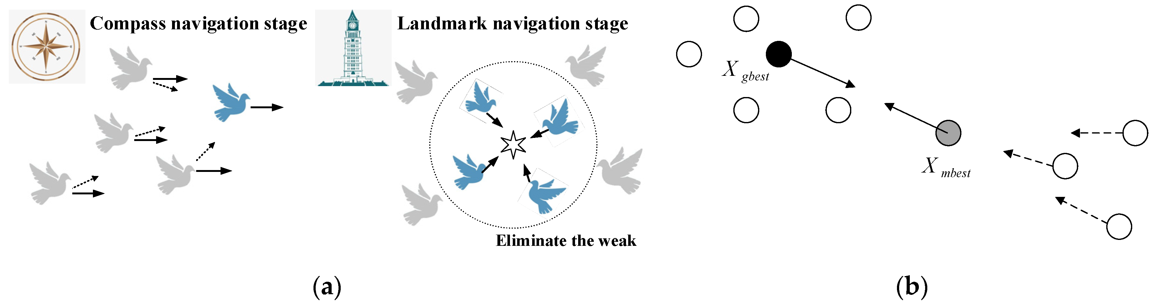
3.2.1. Principle of the Pigeon-Inspired Algorithm

The pigeon-inspired algorithm is a bionic optimization algorithm that finds the combination of parameters at the extremes of the function, according to the set evaluation rules [26]. All parameters are considered as individual “pigeons” that change their positions with certain update rules, and the most suitable combination of values are determined after a certain number of iterations.
During the pre-migration period, pigeons rely on pointing information such as the geomagnetic field and the sun to correct the general direction of their flight. After reaching the vicinity of their destination, they switch to landmark information for navigation. In the whole flock of pigeons, individuals unfamiliar with the map also approach individuals familiar with the landmarks during the movement. Before the start of the optimization search, the velocity information V i and the position information X i of N particles are initialized. Then, two stages of iteration are completed as follows.
A pre-optimal search is navigated by compass operators, and the velocity update of particles is influenced by both the compass information and the optimal individual within the population:
V i N c = V i N c 1 e R × N c + rand ( X best X i N c 1 )
X i N c = X i N c 1 + V i N c
where NC is the current iteration number, Xbest is the optimal particle position information in the current iteration, and R is the compass operator, which can adjust the influence weight of the guide information.
The second stage navigates through the landmark operator. In each iteration, each particle generates an adaptation value based on the set evaluation method, generates the corresponding sequence, and discards the individuals with poor evaluation values by halving the total number of particles to speed up the merit search. The remaining individuals converge to the optimal particle position:
X center N c 1 = i = 1 N X i N c 1 f ( X i N c 1 ) N N c 1 i = 1 N f ( X i N c 1 )
N N c = N N c 1 / 2
X i N c = X i N c + rand ( X center N c 1 X i N c 1 )
where Xcenter is the current particle center position and f(X) is the fitness value of the particle. We used (19) as an evaluation function to calculate the fitness value of the group of particles. A strategy was adopted to complete the calculation, which was simulating the motion after a period of time with the current parameters and robot state quantities, and returning the calculated value of the efficiency during this period. This process is integrated into Figure 3.

3.2.2. Improve PIO by Quantum Rules

Quantum behavior rules play a good role in solving the problems of particle swarm algorithms which are prone to fall into optimality and slow in finding the optimal speed [34]. In this paper, quantum rules are used in the particle position updating process for dynamically decreasing shrinkage. Dilation coefficients A are introduced as compass operators to improve the convergence of the optimal search:
A = ( T N c ) 2 T + 0.5
P = ( rand   1 X pbest i N c 1 + rand   2 X gbest N c 1 ) ( rand   1 + rand   2 )
X i N c = P ± A | X mbest N c 1 X i N c 1 | ln ( 1 / rand )
where T is the number of iterations of the compass operator, Xpbest is the individual historical optimal, Xgbest is the global historical optimal and Xmbest is the individual historical average optimal.
In the landmark operator stage, the landmark operator is changed to a population optimal operator and a learning factor Β is introduced to update the particle information.
B = r o u n d ( 1 + rand )
X new , i = X i N c 1 + rand ( X gbest N c 1 B X mbest N c 1 )
X i N c = { X new , i f ( X new , i ) < f ( X i N c 1 ) X i N c 1 f ( X new , i ) > f ( X i N c 1 )
The corresponding schematic diagram of the algorithm is shown in Figure 4. Under this rule, the particles that are far from the optimal solution first converge to the same position at a rate proportional to the difference between the global historical optimal solution and the individual historical average optimal solution, while expanding the global search degree. Then, the difference between the global historical optimal solution and the individual historical average optimal solution is reduced with the increase of iterations, until the search for the optimal solution is completed and all particles converge to the vicinity of the optimal solution.

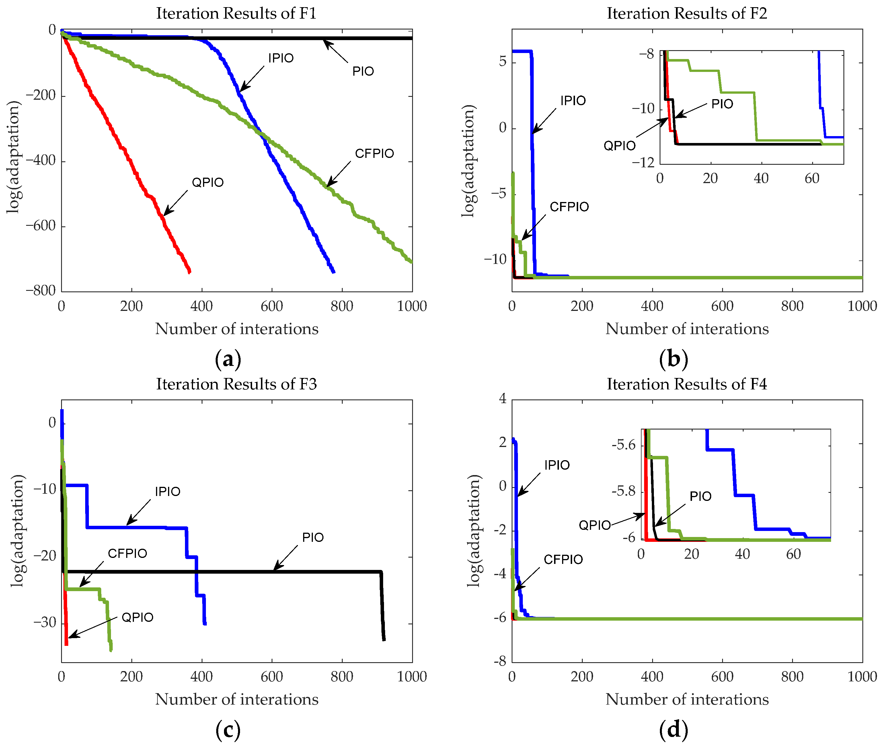
3.2.3. Algorithm Performance Test

To verify the effectiveness of the improved PIO algorithm in this paper, several common test functions were selected for comparing the optimization results of different methods. The relevant contents of the function expressions are shown in Table 1.
Four PIO related algorithms were used to compare convergence speed and convergence accuracy, including two other optimization methods:
(1)
Basic pigeon-inspired algorithm (PIO) [26];
(2)
Improved pigeon-inspired algorithm with inverse and Gaussian factor (IPIO) [35];
(3)
Adaptive pigeon-inspired algorithm with constriction factor (CFPIO) [36];
(4)
Pigeon-inspired algorithm based on quantum behavior rules (QPIO).
The main variables and coefficients in the algorithm were set as: functional dimensions D = 10; number of particle NP = 5 ∗ D; contraction-expansion coefficient A = 1 − 0.5 (degression); compass operator R = 0.5; iteration times of compass T1 = 800; iteration times of landmark T2 = 200 and number of optimization Times = 30.
The optimal solution (Min), the most inferior solution (Max), the average solution (Mean) and the standard deviation (STD) of the results of 30 simulation operations were taken for comparison, and the statistical results are shown in Table 2, and the optimal value is bold. The data of a random optimization process were taken out to plot the convergence process curve, as shown in Figure 5.
From the various statistical results, it can be seen that the proposed algorithm performs better in terms of convergence results and has a greater improvement in the optimization search effect. Besides, under certain test functions, the proposed algorithm can achieve the same optimization results in fewer iterations as other methods with high iterations. For the high real-time parameter requirements of the snake robot, this significantly reduces the computational power requirements of the robot system and provides the possibility of dynamic parameter adjustment in practical applications.

4. Simulation

4.1. Parameters of Robot and Opitimizaion Algorithm

Currently, experiments related to underwater snake robots usually verify the control method through indoor pools, where the robot completes the set motion in still water or in constant irrotational currents. Moreover, physical prototypes are designed so that the robot is subjected to a buoyancy force equal to its own gravity, allowing the robot to move on a horizontal plane to avoid other disturbances. Therefore, the simulation environment set in this paper conforms to the above settings and refers to the friction coefficients c t and c n given by [30], which are often obtained experimentally.
We considered an underwater snake robot with n = 10 links, 2l = 0.14 m length of each link and mass m = 1 kg. The hydrodynamic-related parameters were set as c t = 0.5 , c n = 3 , λ 1 = 0.5 , λ 2 = 20 , and thus c p = 9 . The control parameters were fixed with k P = 20 , k D = 5 ,   k Δ = 100 , and k th = 0.2 . The initial values of the states of the robot were set to 0 or referred to the special instructions.
Some QPIO parameters were adjusted, which was different from the previous section, to D = 3 , N P = 5 × D = 15 , and the number of iterations was reduced to T 1 = 180 , T 2 = 20 . The model proposed in [9] ignores the effect of additional mass forces, which requires that the robot should not be at high speed and that the simplified model is relatively accurate when the rotation of the linkage is below 20 degrees. Therefore, in the later simulations, the gait parameters should be taken in a range of values during the optimization process, which are α [ 0.02 ,   0.06 ] , ω [ 1 ,   2 ] and β [ 0.3 , 0.7 ] .

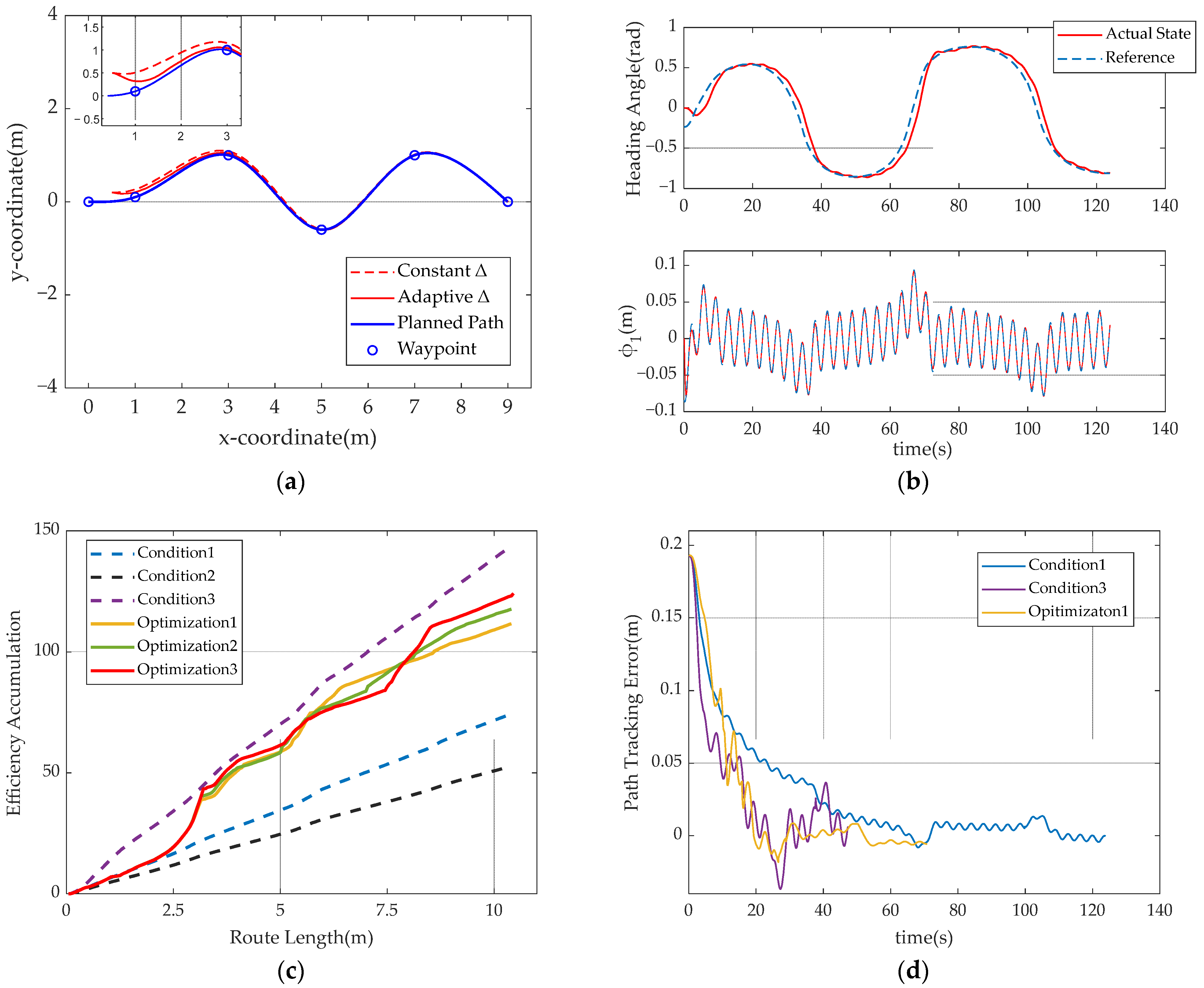
4.2. Path Tracking and Efficiency Optimization

4.2.1. Closed-Loop Curve Path

To highlight the advantages of generating curve functions with the parametric method, a closed-loop curve path was generated using the PCSI method and the waypoints were set at (0, 0), (2, 0), (4.2, 0.5), (3.5, 2.3), (1.6, 1.8) and (0.5, −1), as shown in Figure 6a with the blue circle.
First, three constant gait parameter conditions were set for comparison: (1) Condition 1 for α = 0.04 m , ω = 1.75 and β = 0.52 ; (2) Condition 2 for α = 0.03 m , ω = 2 and β = 0.43 ; (3) Condition 3 for α = 0.06 m , ω = 1.57 and β = 0.7 . These reflect the robot locomotion under different amplitudes and frequencies.
Condition 1 was adopted to verify the tracking effect of the proposed method on the curved path, as shown in Figure 6a,b. It can be seen that the real path and the planned path almost overlapped, so the proposed strategy achieved this task well. It can be seen that the heading angle in Figure 6b has some fluctuations. In fact, the curve bends more when passing the heading point; the robot corrected this after offsetting the planned path slightly.
Then, three optimization simulations with the same conditions were completed to show the efficiency optimization results, avoiding the influence of the algorithm randomness. Figure 6c shows that the three optimizations had the same change trend, and that energy efficiency was significantly improved at the position with larger curvature. The efficiency accumulation was better than the results under Condition 1 and Condition 2, even if the final result was slightly different due to the randomness of the algorithm. This shows that the proposed optimization strategy can reduce the required energy within the same distance. This result may not have been obvious enough and will be further verified in the next simulation.
It seems that there should be a gait pattern that allows the robot to maintain high efficiency, similar to the results under Condition 3. In fact, the robot moves faster with greater amplitude and frequency in this gait pattern, and Figure 6d shows that in this condition, the robot takes only half the time to complete the entire motion. In curved path tracking, there is no need for the robot to move at such a speed, which also increases the tracking error. That is, this increase in efficiency comes at the cost of increased tracking error, and is more pronounced in more complex paths. In the process of optimizing the parameters with QPIO, some unreasonable parameter combinations were removed, for example, the robot can still maintain a high frequency when swinging in the large amplitude. It was too demanding for the robot mechanical system, and a small gait with the speed of only 0.02 m/s was efficient. The reasonable speed of the robot should be around 0.1 m/s–0.2 m/s, according to some experiments. Incidentally, the fluctuation of the tracking error was due to the asymmetric attitude of the robot, where the lateral components of the drag force could not cancel each other out.

4.2.2. Large Curvature Curve Path

To illustrate some inferences in the previous subsection, a path with a greater curvature resembling a sine curve was generated, and the waypoint was set at (0, 0), (1, 0.1), (3, 1), (5, −0.6), (7, 1) and (9, 0), as shown in Figure 7a with the blue circle. Meanwhile, the starting position of robot was set to ( p x ( 0 ) , p y ( 0 ) ) = (0.5, 0.2) to demonstrate the validity of (16). Other conditions were the same as in the previous simulation.
Figure 7a shows that the robot tracked the planned path well under the LOS strategy with the gait of Condition 1, and that the method of (16) can guide the robot to approach the target route faster. The effect of this strategy was more evident in the small window where the start point was set at (0.5, 0.5). In the path of continuous turns, the robot shifted its course more, and this strategy was effective in reducing the tracking error. Figure 7b shows that the robot’s heading angle shifts a little at the turn, but has little effect on the robot in this gait at a slow speed of about 0.09 m/s.
Similarly, three optimization simulations with the same parameters were performed to contrast with the simulation of fixed parameters, as shown in Figure 7c. The efficiency accumulation of the three simulations had a very similar trend in the first period, with the final value varying as the number of optimizations increased, which was caused by the randomness of the algorithm’s choice of parameters. Nevertheless, the results of the optimization strategy were much better than the constant conditions, and the robot efficiency increased significantly for all the large angle turns. The gait of Condition 3 corresponded to a somewhat higher efficiency, but Figure 7d shows that the robot will have a larger tracking error at turns. The speed had some effect on the tracking error, and their error curves were not of the same length; the error curves for all gaits are not recorded in Figure 7d, which would make the results appear confusing.
When the robot deviated from the intended route, a larger linkage offset was calculated by (15), which indirectly led to a change in the control volume in (3), and the efficiency evaluation method (19) proposed in this paper was affected. The energy efficiency was improved by dynamically selecting the gait parameters, while the tracking error did not become large. The dynamic selection of parameters to improve the energy efficiency proposed in this paper is effective while maintaining the path-tracking accuracy.

5. Conclusions

In this paper, curved path-tracking control of an underwater snake robot was investigated, and a commonly used LOS law was used to design the controller. A PCSI method was adopted for path planning, which made the generated path more compatible with the locomotion characteristics of the snake robot. An algorithm improving the PIO with quantum rules was proposed to dynamically select the gait parameters to enhance the energy efficiency of the robot. Simulation results showed that the snake robot can achieve tracking of the planned path with low error, and the intelligent algorithm helps the robot to improve the energy efficiency, especially in the case of large angle turns.
It was found in the simulation that the speed of the robot had a significant impact on the tracking accuracy. In the future, adaptive path tracking controllers will be designed to cope with more complex routes, and to enhance the performance of intelligent algorithms to achieve more stable parameter optimizations. Experiments will be performed to show the validity of the proposed method, along with the development of the physical robot.

Author Contributions

Methodology, B.X., M.J., X.Z., D.Z.; validation, M.J., D.Z.; writing—original draft, M.J., D.Z.; writing—review and editing, B.X., M.J., X.Z.; supervision, B.X., M.J., X.Z. All authors have read and agreed to the published version of the manuscript.

Funding

This research was funded by the National Defense Science and Technology Foundation for Excellent Young Scientist of China, grant number 2020-JCJQ-ZQ-071.

Institutional Review Board Statement

Not applicable.

Informed Consent Statement

Not applicable.

Conflicts of Interest

The authors declare no conflict of interest.

References

  1. Borenstein, J.; Borrell, A. The OmniTread OT-4 serpentine robot. In Proceedings of the 2008 IEEE International Conference on Robotics and Automation, Pasadena, CA, USA, 19–23 May 2008; pp. 1766–1767. [Google Scholar]
  2. Wright, C.; Buchan, A.; Brown, B.; Geist, J.; Schwerin, M.; Rollinson, D.; Tesch, M.; Choset, H. Design and architecture of the unified modular snake robot. In Proceedings of the 2012 IEEE International Conference on Robotics and Automation, Saint Paul, MN, USA, 14–8 May 2012; pp. 4347–4354. [Google Scholar]
  3. Sugita, S.; Ogami, K.; Michele, G.; Hirose, S.; Takita, K. A Study on the Mechanism and Locomotion Strategy for New Snake-Like Robot Active Cord Mechanism—Slime model 1 ACM-S1. J. Robot. Mechatron. 2008, 20, 302–310. [Google Scholar] [CrossRef]
  4. Yamada, H.; Hirose, S. Development of practical 3-dimensional active cord mechanism ACM-R4. J. Robot. Mechatron. 2006, 18, 305–311. [Google Scholar] [CrossRef]
  5. Crespi, A.; Badertscher, A.; Guignard, A.; Ijspeert, A.J. AmphiBot I: An amphibious snake-like robot. Robot. Auton. Syst. 2005, 50, 163–175. [Google Scholar] [CrossRef] [Green Version]
  6. Liljeback, P.; Haugstuen, I.U.; Pettersen, K.Y. Path Following Control of Planar Snake Robots Using a Cascaded Approach. IEEE Trans. Control. Syst. Technol. 2011, 20, 111–126. [Google Scholar] [CrossRef] [Green Version]
  7. Kohl, A.M.; Pettersen, K.Y.; Kelasidi, E.; Gravdahl, J.T. Planar Path Following of Underwater Snake Robots in the Presence of Ocean Currents. IEEE Robot. Autom. Lett. 2016, 1, 383–390. [Google Scholar] [CrossRef] [Green Version]
  8. Zhang, D.; Yuan, H.; Cao, Z. Environmental adaptive control of a snake-like robot with variable stiffness actuators. IEEE/CAA J. Autom. Sin. 2020, 7, 745–751. [Google Scholar] [CrossRef]
  9. Bing, Z.S.; Chen, L.; Chen, G. Towards autonomous locomotion: CPG-based control of smooth 3D slithering gait transition of a snake-like robot. Bioinspiration Biomim. 2017, 12, 035001. [Google Scholar] [CrossRef] [PubMed]
  10. Wang, Z.; Gao, Q.; Zhao, H. CPG-Inspired Locomotion Control for a Snake Robot Basing on Nonlinear Oscillators. J. Intell. Robot. Syst. 2017, 85, 209–227. [Google Scholar] [CrossRef]
  11. Miao, Y.; Gao, F.; Zhang, Y. Gait fitting for snake robots with binary actuators. Sci. China Ser. E Technol. Sci. 2014, 57, 181–191. [Google Scholar] [CrossRef]
  12. Li, D.; Wang, C.; Deng, H.; Wei, Y.; Dongfang, L.; Chao, W.; Hongbin, D. Motion Planning Algorithm of a Multi-Joint Snake-Like Robot Based on Improved Serpenoid Curve. IEEE Access 2020, 8, 8346–8360. [Google Scholar] [CrossRef]
  13. Wang, G.; Yang, W.; Shen, Y.; Shao, H.; Wang, C. Adaptive Path Following of Underactuated Snake Robot on Unknown and Varied Frictions Ground: Theory and Validations. IEEE Robot. Autom. Lett. 2018, 3, 4273–4280. [Google Scholar] [CrossRef]
  14. Borhaug, E.; Pavlov, A.; Pettersen, K.Y. Integral LOS control for path following of underactuated marine surface vessels in the presence of constant ocean currents. In Proceedings of the 47th IEEE Conference on Decision and Control, Cancum, Mexico, 9–11 December 2008; pp. 4984–4991. [Google Scholar]
  15. Wang, X.; Wu, G. Modified LOS Path Following Strategy of a Portable Modular AUV Based on Lateral Movement. J. Mar. Sci. Eng. 2020, 8, 683. [Google Scholar] [CrossRef]
  16. Kelasidi, E.; Pettersen, K.Y.; Liljeback, P.; Gravdahl, J.T. Integral Line-of-Sight for path following of underwater snake robots. In Proceedings of the 2014 IEEE Conference on Control Applications, Antibes, France, 8–10 October 2014. [Google Scholar]
  17. Madhavan, S.; Antonios, T.; Brian, W.; Rafa, B. Co-operative path planning of multiple UAVs using Dubins paths with clothoidarcs. Control. Eng. Pract. 2010, 18, 1084–1092. [Google Scholar]
  18. Jolly, K.; Kumar, R.S.; Vijayakumar, R. A Bezier curve based path planning in a multi-agent robot soccer system without violating the acceleration limits. Robot. Auton. Syst. 2009, 57, 23–33. [Google Scholar] [CrossRef]
  19. Tian, L.; Collins, C. An effective robot trajectory planning method using a genetic algorithm. Mechatronics 2004, 14, 455–470. [Google Scholar] [CrossRef]
  20. Lekkas, A.; Fossen, T.I. Integral LOS Path Following for Curved Paths Based on a Monotone Cubic Hermite Spline Parametrization. IEEE Trans. Control. Syst. Technol. 2014, 22, 2287–2301. [Google Scholar] [CrossRef]
  21. Ariizumi, R.; Matsuno, F. Dynamic Analysis of Three Snake Robot Gaits. IEEE Trans. Robot. 2017, 33, 1075–1087. [Google Scholar] [CrossRef]
  22. Hasanzadeh, S.; Tootoonchi, A.A. Ground adaptive and optimized locomotion of snake robot moving with a novel gait. Auton. Robot. 2010, 28, 457–470. [Google Scholar] [CrossRef]
  23. Wang, Z.F.; Ma, S.G.; Li, B.; Wang, Y.C. Simulation and experimental study of an energy-based control method for the serpentine locomotion of a snake-like robot. Acta Autom. Sin. 2011, 37, 604–614. [Google Scholar]
  24. Cao, Z.; Zhang, D.; Hu, B.; Liu, J. Adaptive Path Following and Locomotion Optimization of Snake-Like Robot Controlled by the Central Pattern Generator. Complexity 2019, 2019, 1–13. [Google Scholar] [CrossRef] [Green Version]
  25. Kelasidi, E.; Jesmani, M.; Pettersen, K.Y.; Gravdahl, J.T. Multi-objective optimization for efficient motion of underwater snake robots. Artif. Life Robot. 2016, 21, 411–422. [Google Scholar] [CrossRef] [Green Version]
  26. Duan, H.; Qiao, P. Pigeon-inspired optimization: A new swarm intelligence optimizer for air robot path planning. Int. J. Intell. Comput. Cybern. 2014, 7, 24–37. [Google Scholar] [CrossRef]
  27. Duan, H.; Huo, M.; Yang, Z.; Shi, Y.; Luo, Q. Predator-Prey Pigeon-Inspired Optimization for UAV ALS Longitudinal Parameters Tuning. IEEE Trans. Aerosp. Electron. Syst. 2019, 55, 2347–2358. [Google Scholar] [CrossRef]
  28. Pei, J.; Su, Y.; Zhang, D. Fuzzy energy management strategy for parallel HEV based on pigeon-inspired optimization algorithm. Sci. China Ser. E Technol. Sci. 2017, 60, 425–433. [Google Scholar] [CrossRef]
  29. Liljeback, P.; Pettersen, K.Y.; Stavdahl, O.; Gravdahl, J.T. Snake Robots: Modelling, Mechatronics, and Control; Springer: London, UK, 2012. [Google Scholar]
  30. Kohl, A.M.; Pettersen, K.Y.; Kelasidi, E.; Gravdahl, J.T. Analysis of underwater snake robot locomotion based on a control-oriented model. In Proceedings of the 2015 IEEE Conference on Robotics and Biomimetics, Zhuhai, China, 6–9 December 2015; pp. 1930–1937. [Google Scholar]
  31. Kelasidi, E.; Liljeback, P.; Pettersen, K.Y.; Gravdahl, T. Innovation in Underwater Robots: Biologically Inspired Swimming Snake Robots. IEEE Robot. Autom. Mag. 2016, 23, 44–62. [Google Scholar] [CrossRef] [Green Version]
  32. Hirose, S. Biologically Inspired Robots: Snake-Like Locomotors and Manipulators; Oxford University Press: London, UK, 1993. [Google Scholar]
  33. Fredriksen, E.; Pettersen, K. Global κ-exponential way-point maneuvering of ships: Theory and experiments. Automatica 2006, 42, 677–687. [Google Scholar] [CrossRef]
  34. Sun, J.; Feng, B.; Xu, W. Particle swarm optimization with particles having quantum behavior. In Proceedings of the 2004 Congress on Evolutionary Computation, Portland, OR, USA, 19–23 June 2004; pp. 325–331. [Google Scholar]
  35. Liu, H.M.; Yan, X.S.; Wu, Q.H. An improved pigeon-inspired optimization algorithm and its application in parameter inversion. Symmetry 2019, 11, 1291. [Google Scholar] [CrossRef] [Green Version]
  36. Guo, R.; Zhao, R.X.; Wu, H.Z.; Ren, D.; Fan, J.W. Adaptive pigeon group algorithm with contraction factor for function optimization. Internet Things Technol. 2017, 7, 91–94. [Google Scholar]
Figure 1. Variables labeling for both models.
Jmse 10 00047 g001
Figure 2. Los guidance diagram: (a) straight path; (b) geometry for curve path.
Jmse 10 00047 g002
Figure 3. Controller Structure and optimization framework.
Jmse 10 00047 g003
Figure 4. PIO principle: (a) Compass and landmark operator model; (b) improved landmark operator model.
Jmse 10 00047 g004
Figure 5. Comparison of optimization performance of various algorithms under different test functions: (a) convergence trend under F1; (b) convergence trend under F2; (c) convergence trend under F3; (d) convergence trend under F4.
Jmse 10 00047 g005
Figure 6. Simulation results of closed-loop curve path: (a) trajectory of the center of mass; (b) heading angle and the joint angle of link 1; (c) efficiency accumulation at different parameters; (d) path tracking error at different gaits.
Jmse 10 00047 g006
Figure 7. Simulation results of a large curvature curve path: (a) trajectory of the center of mass; (b) heading angle and the joint angle of link 1; (c) efficiency accumulation at different parameters; (d) path-tracking error at different gaits.
Jmse 10 00047 g007
Table 1. Test function and condition settings for optimization algorithm.
NumberTest FunctionExpressionsDefinition DomainOptimal Solution
F1Sphere f ( X ) = i = 1 n x i 2 [−100, 100](0, 0)
F2Schwefel f ( X ) = 418.9829 n + i = 1 n [ x i sin ( | x i | ) ] [−500, 500](420.9687, 0)
F3Rastrigin f ( X ) = 10 n + i = 1 n [ x i 2 10 cos ( 2 π x i ) ] [−10, 10](0, 0)
F4Griewangk f ( X ) = 1 4000 i = 1 n x i 2 + i = 1 n cos ( x i i ) + 1 [−600, 600](multi-extreme-points)
Table 2. Result statistics of different algorithms.
FunctionPIOIPIOCFPIOQPIO
F1Mean0.50120.11470.03920
STD0.75830.45220.14890
Min0000
Max3.17242.20730.56810
Time(s)Tmean1.06350.92970.99641.7328
F2Mean2.23680.69551.10020.0785
STD4.88491.60662.70230.2001
Min1.26 × 10−51.26 × 10−51.26 × 10−51.26 × 10−5
Max21.72947.538614.83720.6527
Time(s)Tmean0.96511.03181.02292.0073
F3Mean0.20190.01560.00410
STD0.37660.05990.01440
Min0000
Max1.21090.28660.08320
Time(s)Tmean0.93801.01611.08181.8141
F4Mean0.07860.04410.00480.0042
STD0.13750.11140.00620.0041
Min0.00250.00250.00250.0025
Max0.57030.54820.03530.0239
Time(s)Tmean0.99481.00051.03541.9682
Publisher’s Note: MDPI stays neutral with regard to jurisdictional claims in published maps and institutional affiliations.

