Research on Sailing Efficiency of Hybrid-Driven Underwater Glider at Zero Angle of Attack

Abstract

The sailing efficiency of an underwater glider, an important type of marine environment detection and data collection equipment, directly affects its range and duration. The zero-angle-of-attack gliding can be achieved by adjusting the wing installation angle to minimize the drag and improve the sailing efficiency, and thus further improving performance of the glider. This paper first presents the dynamic characteristics of a hybrid-driven underwater glider with a certain wing installation angle when it is sailing at zero angle of attack in buoyancy-driven mode and hybrid-driven mode. In buoyancy-driven mode, with a given wing installation angle, the glider can achieve zero-angle-of-attack gliding only at a specific glide angle. In hybrid-driven mode, due to the use of a propulsion system, the specific glide angle that allows the zero-angle-of-attack gliding in buoyancy-driven mode is expanded to a glide angle range bounded by zero degrees. Then, the energy consumption per meter is introduced as an indicator of sailing efficiency, and the effects of glide angle and wing installation angle on sailing efficiency of the zero-angle-of-attack glider in two driving modes are studied under the conditions of given net buoyancy and given speed, respectively. Accordingly, the optimal wing installation angle for maximizing the sailing efficiency is proposed. Theoretical analysis shows that the sailing efficiency of a zero-angle-of-attack glider can be higher than that of a traditional glider. Considering the requirements of different measurement tasks, a higher sailing efficiency can be achieved by setting reasonable parameters and selecting the appropriate driving mode.

1. Introduction

Since the concept of an underwater glider was proposed [1], various gliders have been developed globally, and researches on the theory and technology of gliders have been promoted greatly. At present, many underwater gliders have been applied in oceanographic research and coastal survey, among which Slocum [2], Spray [3], and Seaglider [4] are widely recognized. In addition, the diversified novel gliders, including XRay with a high lift-to-drag ratio profile [5], Deepglider with working depth up to 6000 m [6], LUNA disk-type underwater glider for virtual mooring [7], and SeaExplorer with hybrid-driven mode [8], continuously improve and expand the working scope and ability of underwater vehicles.

As is known to all, the drag of a glider has a direct impact on its sailing efficiency. Since the hull of the traditional glider has an inefficient lift surface with low lift-to-drag ratio, it provides far less lift than wings, but its drag accounts for most of the total drag [3,9]. In order to obtain a higher lift-to-drag ratio, the traditional glider with fixed symmetrical wings has to sail at a larger angle of attack, which leads to increased hull drag and reduced economy. Therefore, considering the advantage of higher lift-to-drag ratio of the wing, the angle of attack of the hull can be reduced by designing wings with a certain installation angle, so as to reduce the proportion of hull drag in the total drag and improve the sailing efficiency. When diving, the glider changes the wing installation angle to achieve positive lift. Accordingly, when ascending, it adjusts the wing installation angle to achieve an opposite configuration of the wings. Graver [9] proposed that the hull of the glider can be kept at zero angle of attack by adjusting the wing installation angle to minimize the drag. Chen et al. [10] analyzed the motion characteristics of the hybrid-driven glider in AUV mode, and the simulation results show that the hybrid-driven glider will experience a much lower drag and obtain a higher glide speed in zero angle of attack and neutral buoyancy case. In short, it is an effective way to improve the sailing efficiency of the glider by using the wing with a certain installation angle to achieve zero angle of attack.

In addition, Bachmayer et al. [11] proposed a hybrid-driven glider that integrates AUV technology, which has better maneuverability and mission diversity. The Autosub Long Range AUV [12] overcomes the effects of the net positive buoyancy at low speed with wings, so as to achieve a long range. MBARI’s Tethys [13,14] uses a propeller that allows level flight and a variable speed range of 0.5–1.2 m/s, and the high-endurance operations can be achieved by integrating variable buoyancy devices. Driven by variable buoyancy system and propulsion system, the glider can sail in both buoyancy-driven mode and hybrid-driven mode. In hybrid-driven mode, the propulsion system is turned on, and the glider is jointly driven by thrust and net buoyancy. In this way, the glider with a certain wing installation angle can realize the profile motion and the horizontal flight motion at zero angle of attack. The conceptual design of the zero-angle-of-attack glider with a certain wing installation angle and its motion modes in the vertical plane are shown in Figure 1 and Figure 2.

However, the following issues still need to be solved: how to realize zero-angle-of-attack gliding with different driving modes, how to determine the appropriate wing installation angle to obtain a higher sailing efficiency, whether the introduction of a propulsion system will bring about the reduction of economy, and how to compare the sailing efficiency of a zero-angle-of-attack glider with that of a traditional glider. In view of this, this paper mainly studies the sailing efficiency of zero-angle-of-attack gliders and a theoretical analysis thereof is presented, which is helpful to the overall design and improves the applicability of gliders.

The paper is arranged as follows. In Section 2, the relationship among net buoyancy, thrust, wing installation angle, glide angle, and glide speed is studied by establishing the force balance equations at zero angle of attack in a steady gliding state. The glide angle ranges of the glider sailing at zero angle of attack in buoyancy-driven mode and hybrid-driven mode are obtained, respectively. In Section 3, the energy consumption per meter of horizontal transit is introduced as an indicator of sailing efficiency, and the energy consumption model is established and analyzed under given net buoyancy and glide speed, respectively. The conclusions are presented in Section 4.

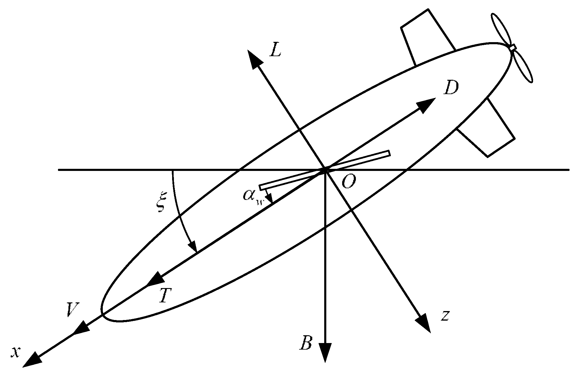
2. Glide Angle Range of the Zero-Angle-of-Attack Glider in Different Driving Modes

Theoretical analysis shows that the glider can only realize zero-angle-of-attack gliding within a specific glide angle range decided by the wing installation angle. Since the upward and downward gliding processes are symmetrical, this paper studies the downward process in a steady gliding state only. Definitions of the variables are shown in the Appendix A at the end of the paper.

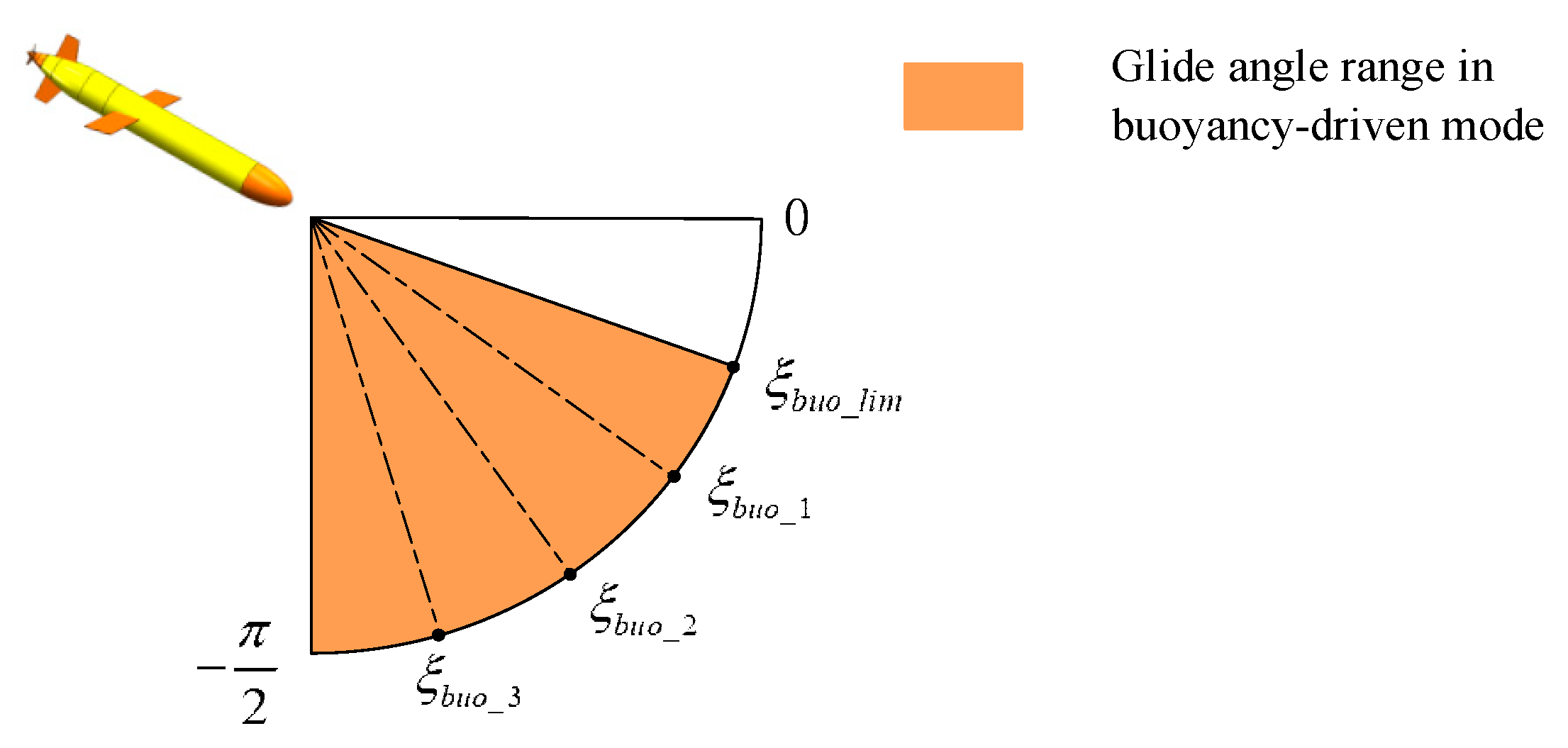
2.1. The Glide Angle Range in Buoyancy-Driven Mode

In buoyancy-driven mode, the net buoyancy is the only driving force, and the propulsion system is turned off. Figure 3 shows the force diagram of the glider diving at zero angle of attack in buoyancy-driven mode. The glide angle $\xi$ is negative during the downward process. Since the net buoyancy is negative in the diving process, the configuration of the wings should be adjusted to achieve force balance and the wing installation angle ${\alpha }_w$ should be no more than $\frac{\pi }{2}$, as shown in Figure 3.

The force balance equations can be obtained through force analysis

$$L\sin \xi +D\cos \xi =0$$

(1)

$$L\cos \xi -D\sin \xi -B=0$$

(2)

From Equations (1) and (2), we have

$$D=-B\sin \xi$$

(3)

$$L=B\cos \xi$$

(4)

Given that the glider usually sails in a steady state at a low glide speed, the lift and drag of the glider are mainly composed of the wing part and the hull part. Since the glider studied in this paper keeps gliding at zero angle of attack, the drag and lift of the two parts can be written, according to the study of Graver [9] and Jenkins et al. [15], as follows:

$$\{\begin{array}{l}{D}_w=\frac{1}{2}\rho S_w\left(C_{d0\_wing}+C_{d\_wing}^{\alpha }{\alpha }_w{}^2\right)V^2\\ L_w=\frac{1}{2}\rho S_w{C}_{l\_wing}^{\alpha }{\alpha }_w{V}^2\\ D_h=\frac{1}{2}\rho S_h{C}_{d0\_hull}{V}^2\\ L_h=0\end{array}$$

(5)

The four hydrodynamic coefficients $C_{d0\_hull}$, $C_{d0\_wing}$, $C_{d\_wing}^{\alpha }$, and $C_{l\_wing}^{\alpha }$ can be obtained through simulation or experiment and are independent of the wing installation angle ${\alpha }_w$.

Considering the coupling between the wings and the hull, a lift correction factor ${\kappa }_L$ is introduced and the lift of the zero-angle-of-attack glider is:

$$L={\kappa }_L{L}_w=\frac{1}{2}\rho S_w{\kappa }_L{C}_{l\_wing}^{\alpha }{\alpha }_w{V}^2$$

(6)

Accordingly, we regard the drag of other parts, such as tail and propeller, as an increment of $D_h$ and introduce a drag correction factor ${\kappa }_D$, then the overall drag acting on the zero-angle-of-attack glider can be written as:

$$D=D_w+{\kappa }_D{D}_h=\frac{1}{2}\rho S_w\left(C_{d0\_wing}+C_{d\_wing}^{\alpha }{\alpha }_w{}^2\right)V^2+\frac{1}{2}\rho S_h{\kappa }_D{C}_{d0\_hull}{V}^2$$

(7)

The correction factors ${\kappa }_L$ and ${\kappa }_D$ are related to shape of the glider, which can be obtained through simulation or experiment [16,17].

Then, by combining Equations (3)–(7), the glide angle in buoyancy-driven mode can be obtained:

$${\xi }_{buo}=-\arctan \frac{X+Y{\alpha }_w{}^2}{Z{\alpha }_w}$$

(8)

where

$$\{\begin{array}{l}X=S_w{C}_{d0\_wing}+S_h{\kappa }_D{C}_{d0\_hull}\\ Y=S_w{C}_{d\_wing}^{\alpha }\\ Z=S_w{\kappa }_L{C}_{l\_wing}^{\alpha }\end{array}$$

(9)

$X$, $Y$, and $Z$ are shape-related parameters, which are greater than zero.

It can be seen from Equation (8) that for a given wing installation angle, the glider can achieve zero-angle-of-attack gliding only at a specific glide angle in buoyancy-driven mode. Furthermore, the glide angle range obtained by adjusting the wing installation angle cannot fully cover the whole area of $\left(-\frac{\pi }{2},0\right]$.

In order to solve the glide angle range in buoyancy-driven mode, Equation (8) is used to obtain the limit glide angle by means of derivation. Let $f({\alpha }_w)=-\frac{X+Y{\alpha }_w{}^2}{Z{\alpha }_w}$, and the partial derivative of ${\alpha }_w$ is determined:

$$\{\begin{array}{l}{\alpha }_w\in \left(0,\sqrt{\frac{X}{Y}}\right),f_{{\alpha }_w}^{\prime }({\alpha }_w)>0\\ {\alpha }_w\in \left(\sqrt{\frac{X}{Y}},\frac{\pi }{2}\right),f_{{\alpha }_w}^{\prime }({\alpha }_w)<0\end{array}$$

(10)

As the wing installation angle ${\alpha }_w$ increases, the glide angle ${\xi }_{buo}$ increases first and then decreases. When $a_w=\sqrt{\frac{X}{Y}}$, the limit glide angle in buoyancy-driven mode can be obtained:

$${\xi }_{buo\_lim}=-\arctan \frac{2\sqrt{XY}}{Z}$$

(11)

It can be seen from Equation (11) that the limit glide angle ${\xi }_{buo\_lim}$ is only related to parameters $X$, $Y$, and $Z$.

Therefore, in buoyancy-driven mode, the glider can sail at zero angle of attack within the glide range of $\left(-\frac{\pi }{2},{\xi }_{buo\_lim}\right]$ with different wing installation angles. As shown in Figure 4, the wing installation angles of the glider are ${\alpha }_{w1}$, ${\alpha }_{w2}$, and ${\alpha }_{w3}$, and let $0<{\alpha }_{w3}<{\alpha }_{w2}<{\alpha }_{w1}<\sqrt{\frac{X}{Y}}$. The corresponding glide angles in buoyancy-driven mode are recorded as ${\xi }_{buo\_1}$, ${\xi }_{buo\_2}$, and ${\xi }_{buo\_3}$, respectively. According to Equation (10), we have $-\frac{\pi }{2}<{\xi }_{buo\_3}<{\xi }_{buo\_2}<{\xi }_{buo\_1}<{\xi }_{buo\_lim}$.

In addition, at any glide angle in the orange area in Figure 4, the glider can realize zero-angle-of-attack gliding with two wing installation angles, among which the smaller one should be selected to obtain a lower drag. The theoretical value range of the wing installation angle should be:

$${\alpha }_w\in \left(0,\sqrt{\frac{X}{Y}}\right]$$

(12)

Furthermore, the glide speed in buoyancy-driven mode can be obtained by Equations (4) and (6):

$$V_{buo}=\sqrt{\frac{2B\cos {\xi }_{buo}}{\rho Z{\alpha }_w}}$$

(13)

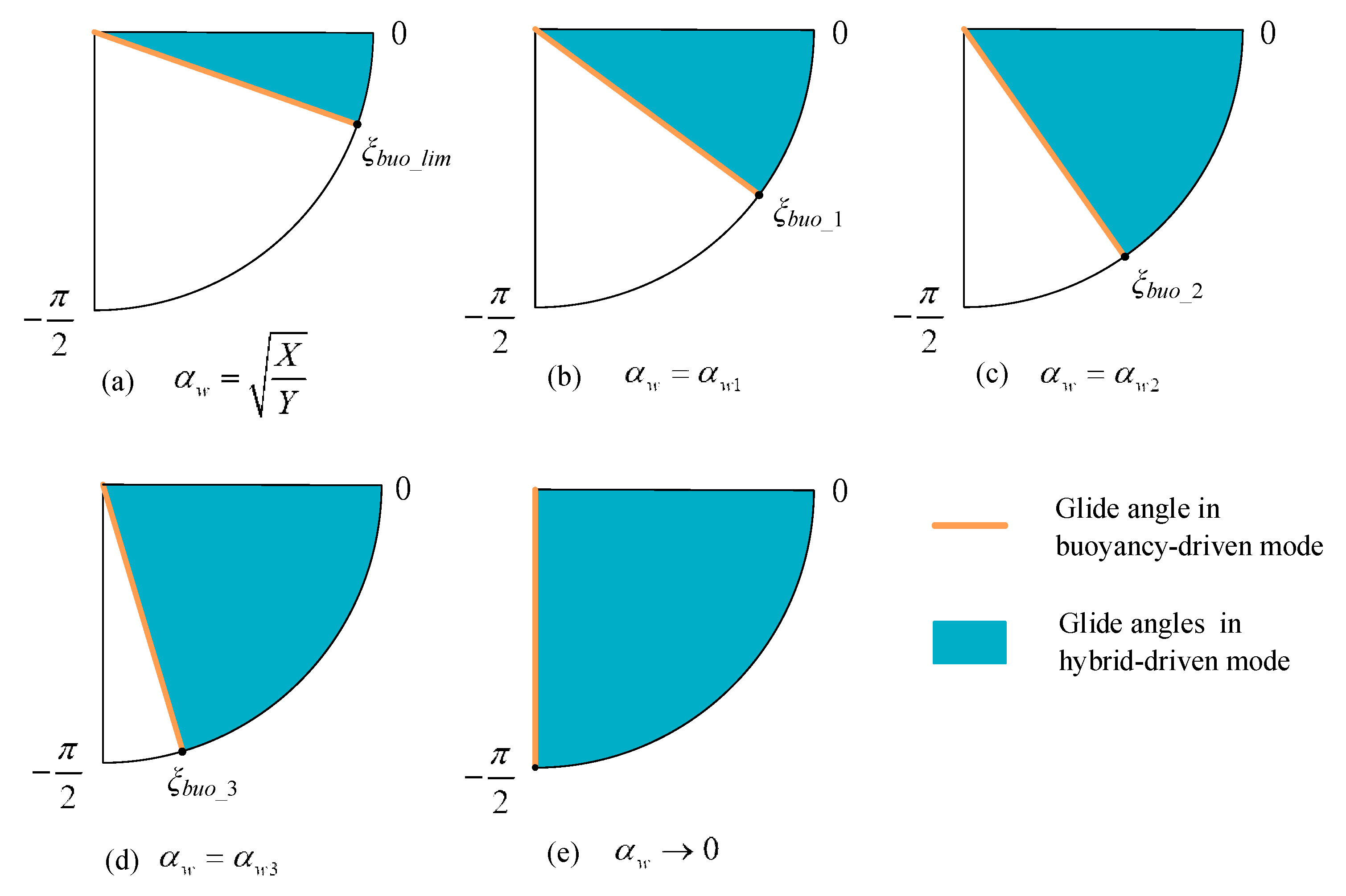
2.2. The Glide Angle Range in Hybrid-Driven Mode

In hybrid-driven mode, the propulsion system is turned on, and the glider is jointly driven by thrust and net buoyancy. Similar to Figure 3, Figure 5 shows the force diagram of the glider diving at zero angle of attack in hybrid-driven mode.

The force balance equations can be obtained through force analysis

$$L\sin \xi +D\cos \xi -T\cos \xi =0$$

(14)

$$L\cos \xi -D\sin \xi -B+T\sin \xi =0$$

(15)

From Equations (14) and (15), we have:

$$D=T-B\sin \xi$$

(16)

$$L=B\cos \xi$$

(17)

The glide speed in hybrid-driven mode can be obtained by Equations (5), (9), and (17):

$$V_{hybrid}=\sqrt{\frac{2B\cos \xi }{\rho Z{\alpha }_w}}$$

(18)

Combine Equations (5), (9), (16), and (18) to obtain the thrust in hybrid-driven mode:

$$T=D+B\sin \xi =\frac{B\cos \xi \left(X+Y{\alpha }_w{}^2\right)}{Z{\alpha }_w}+B\sin \xi$$

(19)

As analyzed in Section 2.1, for a given wing installation angle ${\alpha }_w$, the glider can realize zero-angle-of-attack gliding in buoyancy-driven mode at the glide angle of $-\arctan \frac{X+Y{\alpha }_w{}^2}{Z{\alpha }_w}$. When the propulsion system is turned on, the zero-angle-of-attack glider switches to hybrid-driven mode. At this time, $T>0$ and $\xi >-\arctan \frac{X+Y{\alpha }_w{}^2}{Z{\alpha }_w}$ can be obtained according to Equation (19). That is to say, the glide angle range $\left(-\arctan \frac{X+Y{\alpha }_w{}^2}{Z{\alpha }_w},0\right]$ in hybrid-driven mode can be achieved by adjusting the thrust. The lower limit of this glide angle range is exactly the specific glide angle mentioned above that allows the glider to achieve zero angle of attack in buoyancy-driven mode. In hybrid-driven mode, due to the use of a propulsion system, the specific glide angle in buoyancy-driven mode is expanded to a glide angle range bounded by zero degrees.

In summary, for a given wing installation angle ${\alpha }_w$, the available glide angle range to achieve zero angle of attack is:

$$\xi \in \left[-\arctan \frac{X+Y{\alpha }_w{}^2}{Z{\alpha }_w},0\right]$$

(20)

Besides, by combining Equations (10) and (20), we can see that the available glide angle range is larger with a smaller wing installation angle. As shown in Figure 6, when the zero-angle-of-attack glider sails in buoyancy-driven mode, let $0<{\alpha }_{w3}<{\alpha }_{w2}<{\alpha }_{w1}<\sqrt{\frac{X}{Y}}$, and we can get $-\frac{\pi }{2}<{\xi }_{buo\_3}<{\xi }_{buo\_2}<{\xi }_{buo\_1}<{\xi }_{buo\_lim}$ according to Equation (10). By turning on the propulsion system, the glider switches to hybrid-driven mode and can achieve zero angle of attack in the glide angle ranges of $\left({\xi }_{buo\_1},0\right]$, $\left({\xi }_{buo\_2},0\right]$, and $\left({\xi }_{buo\_3},0\right]$, as indicated by the blue areas of Figure 6b–d. When the wing installation angle approaches zero, the glider can sail at zero angle of attack in hybrid-driven mode in the glide angle range of $\left(-\frac{\pi }{2},0\right]$, as indicated by the blue area of Figure 6e.

For a given wing installation angle, the propulsion system does additional work in hybrid-driven mode, but the zero-angle-of-attack glider sails at a shallower glide angle and travels a longer horizontal distance in a single profile than in buoyancy-driven mode. The sailing efficiency in two driving modes will be compared in Section 3.

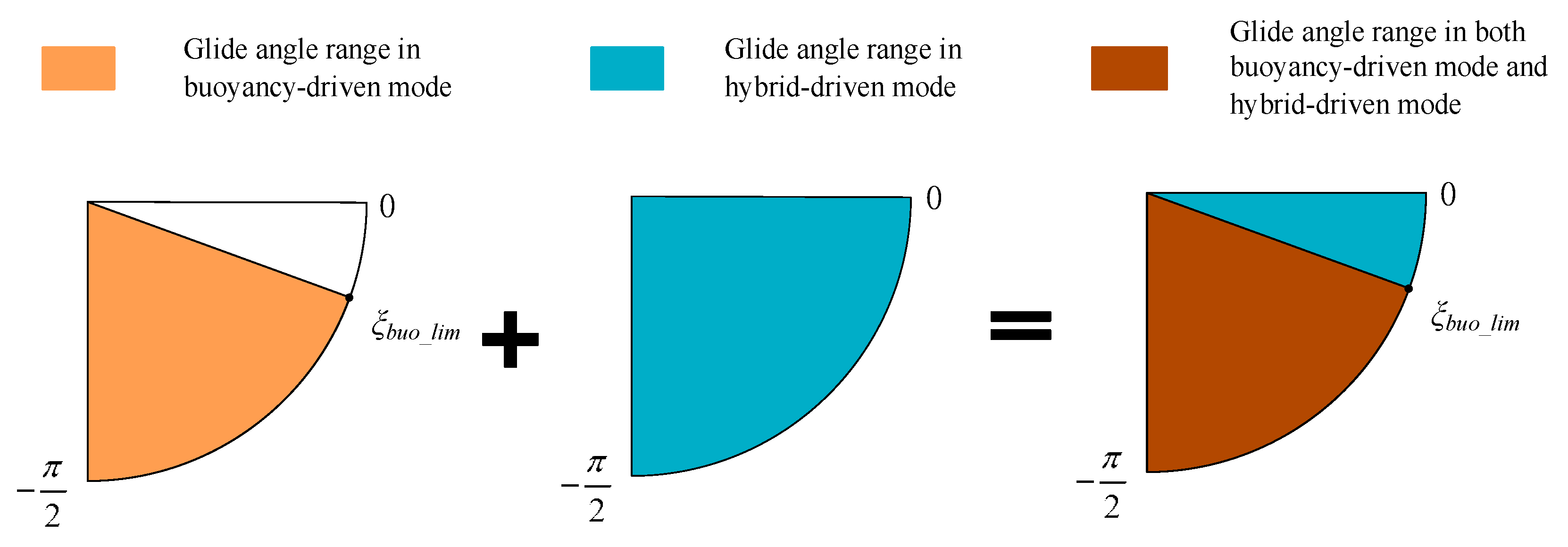
2.3. The Glide Angle Range of the Zero-Angle-of-Attack Glider

According to the above analysis, the glider can sail at zero angle of attack in both buoyancy-driven mode and hybrid-driven mode in the glide angle range of $\left(-\frac{\pi }{2},{\xi }_{buo\_lim}\right]$ by changing the wing installation angle, as indicated by the brown area in Figure 7. However, when $\xi \in \left({\xi }_{buo\_lim},0\right]$, zero-angle-of-attack gliding can only be achieved in hybrid-driven mode, no matter how the wing installation angle is changed. It is worth noting that, according to Equations (10) and (20), the wing installation angle of the zero-angle-of-attack glider in buoyancy-driven mode is larger than that in hybrid-driven mode for any glide angle in the brown area.

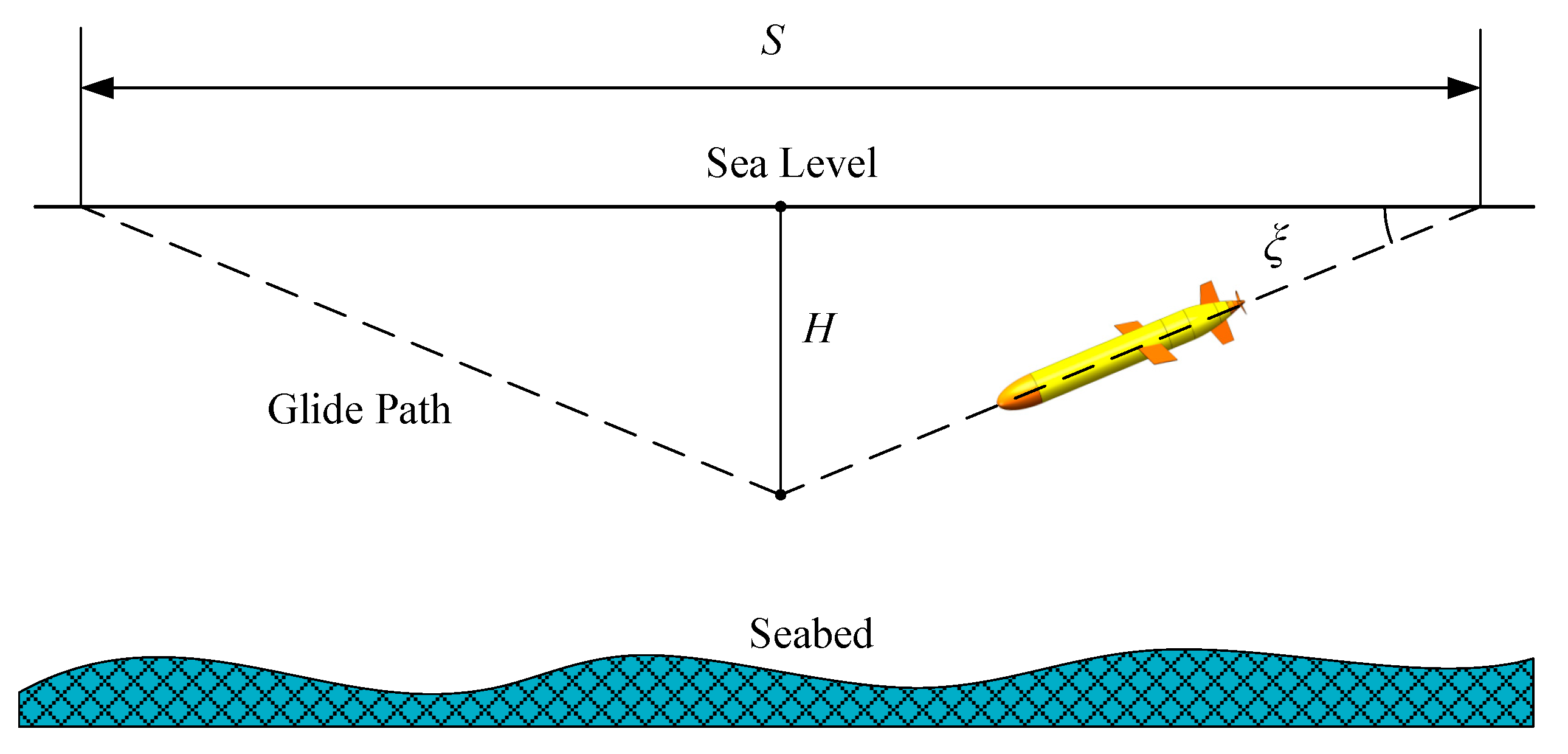
3. Energy Consumption per Meter and Sailing Efficiency

3.1. Energy Consumption Model $e_B-\xi -{\alpha }_w$

In order to establish the relationship among sailing efficiency and dynamic parameters, energy consumption per meter is introduced as an indicator of sailing efficiency [9,18].

The schematic diagram of the glider’s profile motion in the vertical plane is shown in Figure 8.

The horizontal distance of one profile is:

$$S=-2H\cot \xi$$

(21)

The time of the downward process is:

$$t=\frac{-H}{V\sin \xi }$$

(22)

The work done by thrust $T$ of the propulsion system during the downward process can be calculated by combining Equations (19) and (22).

$$W=\frac{TV}{{\eta }_1}t=\frac{-HT}{{\eta }_1\sin \xi }=-\frac{BH}{{\eta }_1}\left(\left(X+Y{\alpha }_w{}^2\right)\frac{\cot \xi }{Z{\alpha }_w}+1\right)$$

(23)

For the variable buoyancy system, ignore the extra energy consumption caused by the thermocline as well as the buoyancy loss caused by the change of seawater density and compression ratios of the hull, and then the buoyancy volume change at the low point of the profile can be computed:

$$\Delta V_L=\frac{2B}{\rho g}$$

(24)

Then, the energy consumption of the variable buoyancy system can be expressed as:

$$W_{buo}=\frac{\rho gH\Delta V_L}{{\eta }_2}=\frac{2BH}{{\eta }_2}$$

(25)

Furthermore, the wing actuator only operates twice in a single profile and its energy consumption is greatly smaller than that of variable buoyancy system and propulsion system. In this regard, the paper does an approximate treatment and ignores the energy loss of the wing actuator.

According to Equations (21), (23), and (25), the energy consumption per meter of the zero-angle-of-attack glider $e_B$ can be calculated:

$$e_B=\frac{2W+W_{buo}}{S}=B\frac{\left(X+Y{\alpha }_w{}^2\right){\eta }_2+\left({\eta }_2-{\eta }_1\right)Z{\alpha }_w\tan \xi }{{\eta }_1{\eta }_{2}Z{\alpha }_w}$$

(26)

Equation (26) contains the net buoyancy term, which is introduced as the energy consumption model $e_B-\xi -{\alpha }_w$. We can see that under given net buoyancy, $\xi$ and ${\alpha }_w$ determine the value of $e_B$. The larger the $e_B$ is, the lower the sailing efficiency will be.

3.1.1. Discussion on the Efficiency of Two Driving Systems

Equation (26) contains both the efficiency of the propulsion system ${\eta }_1$ and the efficiency of the variable buoyancy system ${\eta }_2$. The efficiency of the propulsion system is the ratio of the power for overcoming drag to the electrical input power [19], as shown in Equation (27):

$${\eta }_1=\frac{DV}{U_1{I}_1}=\frac{T{V}_A\left(1-\tau \right)}{U_1{I}_1\left(1-w\right)}$$

(27)

The efficiency of the propulsion system mainly depends on the efficiency of propeller and dynamic seal. According to the propeller theory, it is easier to obtain a higher efficiency by adopting a two-blade open water propeller with a large diameter, whose efficiency can reach over 70%. Examples can be found in the Kongsberg Hugin 1000 AUV and the ISE Explorer AUV. In addition, the ducted propeller has a larger thrust at a low speed, but its efficiency is generally significantly lower than that of an open water propeller, making it suitable for situations with external power supply and heavy loads, such as ROV (remote operated vehicle).

As for the dynamic seal, there are three common ways: pressure compensation seal, O-ring seal, and magnetic coupling seal. The pressure compensation seal uses a compensator to balance outer pressure, and the viscous losses significantly reduce the efficiency, so it is generally used for a deep-sea propulsion system. The O-ring seal requires a simple structure, but the friction between the O-ring and the shaft consumes a lot of power under the deep water pressure, so it is suitable for application in shallow water within a few hundred meters. The magnetic coupling seal has a more complex structure and a larger self-weight, but it has a high reliability and the efficiency is not affected by the working depth. The MBARI’s Tethys adopts a two-blade open water propeller and a magnetic coupling seal, and the measured efficiency and expected efficiency of its propulsion system are 49% and 53%, respectively [14]. The Autosub Long Range AUV adopts a single-blade open water propeller and a magnetic coupling seal, whose working depth and propulsion efficiency are 6000 m and 38%, respectively [12].

Accordingly, the efficiency of the variable buoyancy system ${\eta }_2$ mainly depends on the efficiency of the pump, which overcomes outer pressure to discharge oil and causes the volume change of the bladder, thus generating net buoyancy. It is the ratio of the mechanical output power (pressure times rate of volume change) to the electrical input power [4], as shown in Equation (28):

$${\eta }_2=\frac{\rho gH\Delta V_L/t_{oil}}{U_2{I}_2}=\frac{2BH/t_{oil}}{U_2{I}_2}$$

(28)

The actual efficiency of the variable buoyancy system for a glider is 50% at depth [20]. Such efficiency for Spray and Seaglider is 40% at 1000 dbar, and that for Slocum Battery is 50% [21]. As analyzed above, with a reasonable design, the propulsion system can obtain an efficiency equivalent to that of the variable buoyancy system. Furlong et al. [22] also pointed out that the efficiency of the propulsion system composed of electric motors and propellers can be comparable with that of variable buoyancy system.

Furthermore, in cases that require a horizontal translation only, the energy needed to propel a traditional neutrally-buoyant AUV will be less than the energy consumed by the variable buoyancy system for the glider with a zigzag course to travel the same voyage [23]. Taking Slocum glider as an example, Hockley and Butka [24] compared the energy consumption of the glider driven by the variable buoyancy system with the propulsion system to achieve the same profile. The result shows that the energy consumption of the glider driven by the propulsion system is only 82% of that driven by the variable buoyancy system.

In brief, it is easier to achieve lower energy consumption and higher efficiency by using a propulsion system than a variable buoyancy system. In other words, as long as a reasonable design is adopted, the propulsion system will have an advantage over the variable buoyancy system in terms of efficiency, that is, ${\eta }_1>{\eta }_2$.

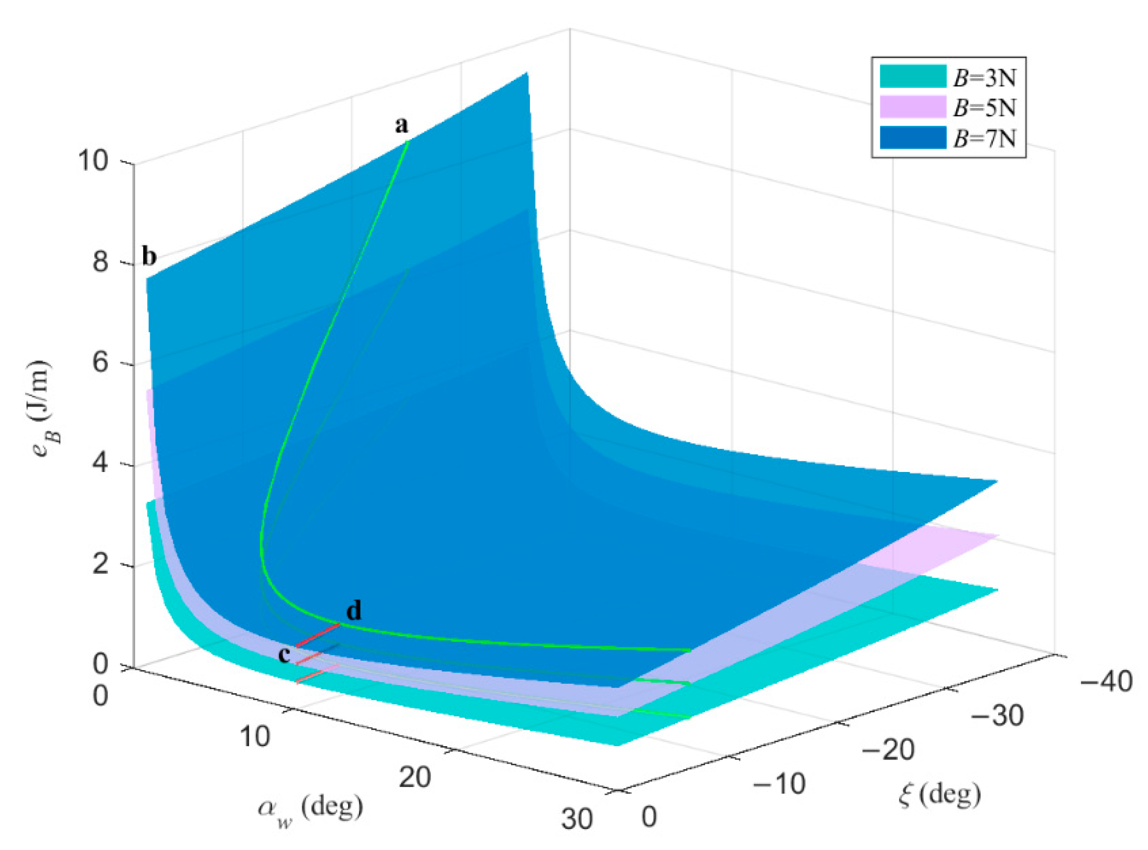
3.1.2. The Influence of Wing Installation Angle on $e_B$ under Given Net Buoyancy

In order to study how the wing installation angle affects $e_B$, the partial derivative of Equation (26) with respect to ${\alpha }_w$ is obtained:

$$e_{B\_{\alpha }_w}^{\prime }=\frac{B\left(Y{\alpha }_w^2-X\right)}{{\eta }_{1}Z{\alpha }_w^2}$$

(29)

It achieves:

$$\{\begin{array}{l}{\alpha }_w\in \left(0,\sqrt{\frac{X}{Y}}\right),e_{B\_{\alpha }_w}^{\prime }<0\\ {\alpha }_w\in \left(\sqrt{\frac{X}{Y}},\frac{\pi }{2}\right),e_{B\_{\alpha }_w}^{\prime }>0\end{array}$$

(30)

According to Equation (30), there exists an optimal installation angle ${\alpha }_{opt}$ which minimizes $e_B$, as:

$${\alpha }_{opt}=\sqrt{\frac{X}{Y}}$$

(31)

The optimal installation angle ${\alpha }_{opt}$ is determined by intermediate values $X$ and $Y$ only, independent of glide angle, net buoyancy, and glide speed. According to Equation (12), ${\alpha }_{opt}$ is just the upper limit of the theoretical value range of wing installation angle.

As analyzed in Section 2.3, for a glide angle that can be used in both modes to achieve zero angle of attack, the corresponding wing installation angle in buoyancy-driven mode is larger than that in hybrid-driven mode. Therefore, according to Equations (12) and (30), the zero-angle-of-attack glider has a higher sailing efficiency in buoyancy-driven mode than in hybrid-driven mode under given net buoyancy at the same glide angle.

In summary, at the same glide angle, according to Equations (13), (18), and (19), the zero-angle-of-attack glider with given net buoyancy can obtain a wider speed range in hybrid-driven mode than in buoyancy-driven mode by adjusting the wing installation angle and thrust, which better meets certain mission requirements, such as in dealing with the current. However, if there is a demand for lower energy consumption and a higher sailing efficiency, the propulsion system can be turned off, and the zero-angle-of-attack glider can adopt the buoyancy-driven mode at the same glide angle by adjusting the wing installation angle. Furthermore, the buoyancy-driven mode of the glider with given net buoyancy can be used to avoid the influence of propulsion noise when acoustic sensors are onboard. Appropriate driving mode should be adopted considering the specific measurement task.

3.1.3. The Influence of Glide Angle on $e_B$ under Given Net Buoyancy

According to Equation (26), the partial derivative of glide angle $\xi$ is obtained:

$$e_{B\_\xi }^{\prime }=\frac{B\left({\eta }_2-{\eta }_1\right){\sec }^2\xi }{{\eta }_1{\eta }_2}$$

(32)

Combined with the analysis of Section 3.1.1, since ${\eta }_1>{\eta }_2$, then $e_{B\_\xi }^{\prime }<0$. As mentioned in Section 2.2, when the wing installation angle remains unchanged, such as keeping at the optimal installation angle, $e_B$ decreases with $\left|\xi \right|$ under given net buoyancy. That is to say, compared with the situation in buoyancy-driven mode, the zero-angle-of-attack glider in hybrid-driven mode has a higher sailing efficiency in this situation, although the propulsion system is turned on, since the increased horizontal range will compensate for the additional energy cost.

For a better understanding, the paper introduces a glider model with traditional layout to illustrate the above analysis [25]. The diameter of the model is 0.2 m and the hull length is 1.5 m. The wings have a NACA0009 airfoil with a chord length of 0.25 m and a wingspan of 1.5 m. The efficiency of the propulsion system ${\eta }_1$ is set to 40%, and the efficiency of the variable buoyancy system ${\eta }_2$ is set to 35%, both of which are obtained experimentally. The net buoyancy is set to 3 N, 5 N, and 7 N as reference and the relevant parameters are:

$$\{\begin{array}{l}{C}_{l\_wing}^{\alpha }=0.0710075\\ C_{d\_wing}^{\alpha }=0.00030777\\ C_{d0\_hull}=0.1009\\ C_{d0\_wing}=0.01826\\ S_w=0.325\\ S_h=0.0314\\ {\kappa }_L=1.12407\\ {\kappa }_D=1.0\end{array}$$

(33)

The $e_B-\xi -{\alpha }_w$ relationship under given net buoyancy can be obtained by combining Equations (9), (26), and (33), as indicated by the area enclosed by points a, b, c, and d in Figure 9. The green line denotes the $e_B-\xi -{\alpha }_w$ relationship in buoyancy-driven mode, and the rest of the area shows the $e_B-\xi -{\alpha }_w$ relationship in hybrid-driven mode. It can be seen that the overall efficiency change under different control quantities is the same. The zero-angle-of-attack glider shares a same optimal installation angle for minimizing energy consumption per meter in the two driving modes, as indicated by the red line. When sharing a same wing installation angle, the zero-angle-of-attack glider has a lower value of energy consumption per meter in hybrid-driven mode than in buoyancy-driven mode, while the contrary is the case when sharing a same glide angle. These are consistent with the theoretical analysis above.

3.2. Energy Consumption Model $e_V-\xi -{\alpha }_w$

If hotel loads and time-based costs dominate the cost of task, the fastest glide possible is desirable [9]. High glide speed could also be important for applications in areas with high currents, such as littoral areas. Therefore, in addition to the net buoyancy, the glide speed is also a common design condition to be given previously. This section studies the energy consumption model $e_V-\xi -{\alpha }_w$ under given speed.

By combining Equations (13) and (18), the required net buoyancy under given speed is:

$$B=\frac{\rho Z{\alpha }_w{V}^2}{2\cos \xi }$$

(34)

The thrust can be obtained by substituting Equation (34) into Equation (19):

$$T=\left(Y{\alpha }_w{}^2+Z{\alpha }_w\tan \xi +X\right)\frac{\rho V^2}{2}$$

(35)

Then, the energy consumption per meter of the zero-angle-of-attack glider $e_V$ can be calculated by combining Equations (26) and (34):

$$e_V=\frac{\left(X+Y{\alpha }_w{}^2\right){\eta }_2+\left({\eta }_2-{\eta }_1\right)Z{\alpha }_w\tan \xi }{2\cos \xi {\eta }_1{\eta }_2}\rho V^2$$

(36)

Equation (36) contains the speed term, which is introduced as the energy consumption model $e_V-\xi -{\alpha }_w$.

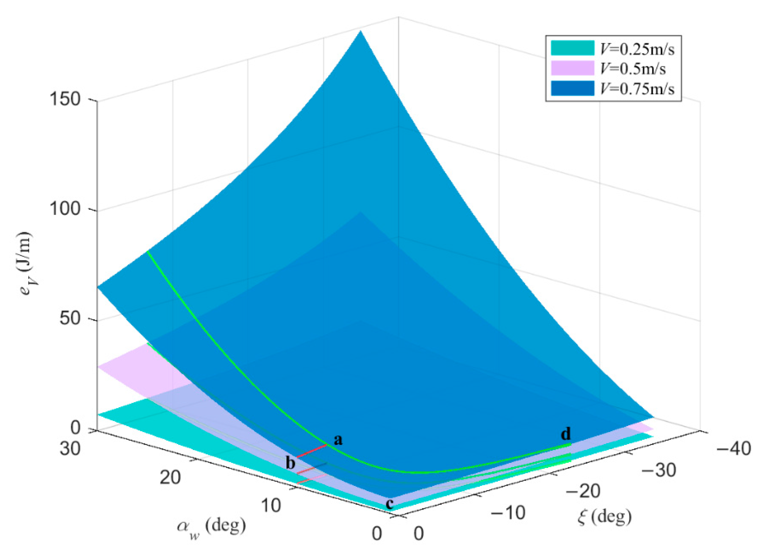
3.2.1. The Influence of Wing Installation Angle on $e_V$ under Given Speed

To explore the influence of wing installation angle on $e_V$, the partial derivative of Equation (36) with respect to ${\alpha }_w$ is obtained:

$$e_{V\_{\alpha }_w}^{\prime }=\frac{\rho V^2\sec \xi \left(2{\alpha }_{w}Y{\eta }_2-\left({\eta }_1-{\eta }_2\right)Z\tan \xi \right)}{2{\eta }_1{\eta }_2}$$

(37)

Since ${\eta }_1>{\eta }_2$, $e_{V\_{\alpha }_w}^{\prime }>0$, at the same glide angle, $e_V$ decreases with ${\alpha }_w$ under given speed, different from the situation under given net buoyancy analyzed in Section 3.1.2. That is, the zero-angle-of-attack glider has a higher sailing efficiency in hybrid-driven mode than in buoyancy-driven mode under given speed at the same glide angle.

It is worth noting that under given net buoyancy, the wing installation angle must always be greater than zero to produce a lift that balances the net buoyancy. If the wing installation angle is set to zero, it is the same case as the traditional glider. Due to the existence of net buoyancy, the traditional glider cannot achieve zero-angle-of-attack gliding. In particular, if the net buoyancy is exactly zero at a given speed, according to Equation (34), the wing installation angle is zero. At this time, only the propulsion system works and the zero-angle-of-attack glider switches to a propulsion mode similar to that of AUV (autonomous underwater vehicle). According to Equations (36) and (37), when the wing installation angle is zero, the energy consumption per meter is the minimum, as shown in Equation (38):

$$e_{propulsion}=\frac{\rho X{V}^2}{2{\eta }_1\cos \xi }$$

(38)

That is to say, under given speed, compared with the situation in buoyancy-driven mode and hybrid-driven mode, the zero-angle-of-attack glider has the highest sailing efficiency in propulsion mode when sailing at the same glide angle.

3.2.2. The Influence of Glide Angle on $e_V$ under Given Speed

According to Equation (36), the partial derivative of glide angle $\xi$ is obtained:

$$e_{V\_\xi }^{\prime }=\frac{\rho V^2{\sec }^3\xi \left(Z{\alpha }_w\left({\eta }_2-{\eta }_1\right)\left(3-\cos 2\xi \right)+\left(X+Y{\alpha }_w^2\right){\eta }_2\sin 2\xi \right)}{4{\eta }_1{\eta }_2}$$

(39)

Since ${\eta }_1>{\eta }_2$, $e_{V\_\xi }^{\prime }<0$, similar to the analysis in Section 3.1.3, when the wing installation angle remains unchanged, the zero-angle-of-attack glider has a higher sailing efficiency in hybrid-driven mode than in buoyancy-driven mode under given speed.

The $e_V-\xi -{\alpha }_w$ relationship can be obtained by combining Equations (9), (33), and (36), as indicated by the area enclosed by points a, b, c, and d in Figure 10. The glide speed is set to 0.25 m/s, 0.5 m/s, and 0.75 m/s as reference. The green line denotes the $e_V-\xi -{\alpha }_w$ relationship in buoyancy-driven mode, and the rest of the area shows the $e_V-\xi -{\alpha }_w$ relationship in hybrid-driven mode. The wing installation angle corresponding to the red line is the upper limit of the theoretical value range of the wing installation angle. It can be seen that different from the situation under given net buoyancy, the zero-angle-of-attack glider has a higher sailing efficiency in hybrid-driven mode than in buoyancy-driven mode at a given speed, whether the glider keeps the same glide angle or the same wing installation angle. Under given net buoyancy, the zero-angle-of-attack glider has the highest sailing efficiency at the wing installation angle $\sqrt{\frac{X}{Y}}$, regardless of the buoyancy-driven mode or the hybrid-driven mode. On the contrary, at a given speed, the glider has the lowest sailing efficiency at the wing installation angle $\sqrt{\frac{X}{Y}}$. The sailing efficiency of the glider in propulsion mode is the highest in this situation, which is consistent with the analysis in Section 3.2.1. Considering the requirements of different measurement tasks, a higher sailing efficiency can be achieved by setting reasonable parameters and selecting the appropriate driving mode.

3.3. Summary and Discussion

As mentioned above, the modes that make a higher sailing efficiency in different conditions can be summarized in

Table 1. The modes that make a higher sailing efficiency in different conditions.

Condition	Given Net Buoyancy B	Given Glide Speed V
Given glide angle $\xi$	Buoyancy-driven mode	Propulsion mode
Given wing installation angle ${\alpha }_w$	Hybrid-driven mode	Hybrid-driven mode

.

As is known, the traditional glider relies only on the variable buoyancy system to change its buoyancy, and realizes the profile gliding motion with the attitude adjustment device. It is impossible for the traditional glider to glide at zero angle of attack with net buoyancy due to the symmetrical wing without installation angle. According to Equations (21) and (25), the energy consumption per meter of traditional glider $e_{traditional}$ can be calculated:

$$e_{traditional}=\frac{W_{buo}}{S}=-\frac{B}{{\eta }_2\cot \xi }$$

(40)

Under the same net buoyancy, the zero-angle-of-attack glider in buoyancy-driven mode has the same sailing efficiency as the traditional glider when sailing at a same glide angle, which can be seen from the comparison between Equations (26) and (40). However, the former has lower drag and higher glide speed. Since the net buoyancy has already met the requirement of zero-angle-of-attack gliding at the given glide angle, the propulsion system of the zero-angle-of-attack glider will do additional work when the glider switches to hybrid-driven mode by adjusting the wing installation angle and maintains the given glide angle. This further leads to the lower sailing efficiency but higher speed compared with the traditional glider.

Accordingly, with a same given glide speed, the zero-angle-of-attack glider in buoyancy-driven mode has a higher sailing efficiency than the traditional glider when sailing at a same glide angle, due to that the drag and the required net buoyancy of the former are lower. Furthermore, according to the analysis in Section 3.2.1, the zero-angle-of-attack glider has a higher efficiency in hybrid-driven mode than in buoyancy-driven mode in this situation. Therefore, regardless of the driving mode, the zero-angle-of-attack glider always has a higher sailing efficiency than a traditional glider under given speed at the same glide angle, as shown in

Table 2. Comparison of the zero-angle-of-attack glider’s sailing efficiency with traditional glider at the same glide angle.

	Condition	Given Net Buoyancy B	Given Glide Speed V
Driving Mode
Buoyancy-driven mode		Equal	Higher
Hybrid-driven mode		Lower	Higher

.

4. Conclusions

This paper mainly studied the realization conditions of zero angle of attack gliding and the sailing efficiency of zero-angle-of-attack glider from a theoretical perspective. Due to the use of a propulsion system, the specific glide angle in buoyancy-driven mode is expanded to a glide angle range bounded by zero degrees. Compared with the traditional glider, the zero-angle-of-attack glider has a higher sailing efficiency at the same speed and glide angle. It is a future plan of our team to develop an engineering prototype and conduct sea trials. The specific conclusions are summarized as follows.

• At a given wing installation angle ${\alpha }_w$, the available glide angle range for a hybrid-driven glider to achieve zero-angle-of-attack gliding is $\xi \in \left[-\arctan \frac{X+Y{\alpha }_w{}^2}{Z{\alpha }_w},0\right]$. In buoyancy-driven mode, the glide angle corresponding to the wing installation angle ${\alpha }_w$ is exactly the lower limit of the range. In hybrid-driven mode, the glide angle range $\left(-\arctan \frac{X+Y{\alpha }_w{}^2}{Z{\alpha }_w},0\right]$ can be achieved by adjusting the thrust.
• Under given net buoyancy and glide angle, the zero-angle-of-attack glider has a wider speed range but a lower sailing efficiency in hybrid-driven mode than in buoyancy-driven mode.
• Under given speed and glide angle, the zero-angle-of-attack glider has a higher sailing efficiency in hybrid-driven mode than in buoyancy-driven mode.
• When the wing installation angle is determined, the zero-angle-of-attack glider will have a higher sailing efficiency in hybrid-driven mode than in buoyancy-driven mode, under both given net buoyancy and given speed.

References

1. Stommel, H. The slocum mission. Oceanography 1989, 2, 22–25. [Google Scholar] [CrossRef]
2. Webb, D.C.; Simonetti, P.J.; Jones, C.P. SLOCUM: An underwater glider propelled by environmental energy. IEEE J. Ocean. Eng. 2001, 26, 447–452. [Google Scholar] [CrossRef]
3. Sherman, J.; Davis, R.E.; Owens, W.B.; Valdes, J. The autonomous underwater glider “Spray”. IEEE J. Ocean. Eng. 2001, 26, 437–446. [Google Scholar] [CrossRef] [Green Version]
4. Eriksen, C.C.; Osse, T.J.; Light, R.D.; Wen, T.; Lehman, T.W.; Sabin, P.L.; Ballard, J.W.; Chiodi, A.M. Seaglider: A long-range autonomous underwater vehicle for oceanographic research. IEEE J. Ocean. Eng. 2001, 26, 424–436. [Google Scholar] [CrossRef] [Green Version]
5. D’Spain, G.L.; Jenkins, S.A.; Zimmerman, R.; Luby, J.C.; Thode, A.M. Underwater acoustic measurements with the Liberdade/X-Ray flying wing glider. J. Acoust. Soc. Am. 2005, 117, 2624. [Google Scholar] [CrossRef]
6. Osse, T.J.; Eriksen, C.C. The deepglider: A full ocean depth glider for oceanographic research. In Proceedings of the Oceans-2007, Vancouver, BC, Canada, 29 September–4 October 2007. [Google Scholar] [CrossRef]
7. Nakamura, M.; Hyodo, T.; Koterayama, W. LUNA testbed vehicle for virtual mooring. In Proceedings of the Seventeenth International Offshore and Polar Engineering Conference, Lisbon, Portugal, 1–6 July 2007. [Google Scholar]
8. Claustre, H.; Beguery, L.; Patrice, P.L.A. SeaExplorer Glider Breaks Two World Records Multisensor UUV Achieves Global Milestones for Endurance, Distance. Sea Technol. 2014, 55, 19–22. [Google Scholar]
9. Graver, J.G. Underwater gliders: Dynamics, Control, and Design. Ph.D. Thesis, Princeton University, Princeton, NJ, USA, 2005. [Google Scholar]
10. Chen, Z.; Yu, J.; Zhang, A.; Song, S. Control system for long-range survey hybrid-driven underwater glider. In Proceedings of the OCEANS-2015—Genova, Genova, Italy, 18–21 May 2015. [Google Scholar] [CrossRef]
11. Bachmayer, R.; Leonard, N.E.; Graver, J.; Fiorelli, E.; Bhatta, P.; Paley, D. Underwater gliders: Recent developments and future applications. In Proceedings of the 2004 International Symposium on Underwater Technology, Taipei, Taiwan, 20–23 April 2004. [Google Scholar] [CrossRef] [Green Version]
12. Furlong, M.E.; Paxton, D.; Stevenson, P.; Pebody, M.; Mcphail, S.D.; Perrett, J. Autosub Long Range: A Long Range Deep Diving AUV for Ocean Monitoring. In Proceedings of the 2012 IEEE/OES Autonomous Underwater Vehicles (AUV), Southampton, UK, 24–27 September 2012. [Google Scholar] [CrossRef]
13. Hobson, B.W.; Bellingham, J.G.; Kieft, B.; McEwen, R.; Godin, M.; Zhang, Y. Tethys-class long range AUVs—Extending the endurance of propeller-driven cruising AUVs from days to weeks. In Proceedings of the 2012 IEEE/OES Autonomous Underwater Vehicles (AUV), Southampton, UK, 24–27 September 2012. [Google Scholar] [CrossRef]
14. Bellingham, J.G.; Zhang, Y.; Kerwin, J.E.; Erikson, J.; Hobson, B.; Kieft, B.; Godin, M.; McEwen, R.; Hoover, T.; Paul, J.; et al. Efficient propulsion for the Tethys long-range autonomous underwater vehicle. In Proceedings of the 2010 IEEE/OES Autonomous Underwater Vehicles, Monterey, CA, USA, 1–3 September 2010. [Google Scholar] [CrossRef]
15. Jenkins, S.A.; Humphreys, D.E.; Sherman, J.; Osse, J.; Jones, C.; Leonard, N.; Graver, J.; Bachmayer, R.; Clem, T.; Carroll, P.; et al. Underwater Glider System Study. Scripps Institution of Oceanography Technical Report. 2003. Available online: https://escholarship.org/uc/item/1c28t6bb (accessed on 15 December 2021).
16. Wolowicz, C.H.; Yancey, R.B. Longitudinal Aerodynamic Characteristics of Light, Twin-Engine, Propeller-Driven Airplanes; NASA Technical Note, 1972. Available online: https://www.nasa.gov/centers/dryden/pdf/87800main_H-646.pdf (accessed on 15 December 2021).
17. Editorial Board of “Aeronautical Aerodynamics Manual”. Aviation Aerodynamics Manual; National Defense Industry Press: Beijing, China, 1983; Volume 2. [Google Scholar]
18. Tian, X.; Zhang, L.; Zhang, H.; Wang, Y.; Liu, Y.; Yang, Y.; Song, L. The Optimal Lift–Drag Ratio of Underwater Glider for Improving Sailing Efficiency. IEEE J. Ocean. Eng. 2021, 46, 808–816. [Google Scholar] [CrossRef]
19. Zhang, Z.; Hu, Z. Ship Propulsion, 1st ed.; National Defense Industry Press: Beijing, China, 1980. [Google Scholar]
20. Griffiths, G. Technology and Applications of Autonomous Underwater Vehicles; CRC Press: Boca Raton, FL, USA, 2002; Volume 2. [Google Scholar]
21. Davis, R.E.; Eriksen, C.C.; Jones, C.P. Autonomous buoyancy-driven underwater gliders. In Technology and Applications of Autonomous Underwater Vehicles; Griffiths, G., Ed.; Taylor & Francis: London, UK, 2002; Chapter 3; pp. 37–58. [Google Scholar]
22. Furlong, M.E.; Mcphail, S.D.; Stevenson, P. A concept design for an ultra-long-range survey class AUV. In Proceedings of the IEEE Oceans 2007—Europe, Aberdeen, UK, 18–21 June 2007. [Google Scholar] [CrossRef] [Green Version]
23. Miller, T.F. A bio-inspired climb and glide energy utilization strategy for undersea vehicle transit. Ocean. Eng. 2018, 149, 78–94. [Google Scholar] [CrossRef]
24. Hockley, C.; Butka, B. Can a Conventional Propulsion System Match the Efficiency of an Underwater Glider Buoyancy Engine? Mar. Technol. Soc. J. 2019, 53, 75–82. [Google Scholar] [CrossRef]
25. Hu, R. Research on the Motion of Underwater Glider in Vertical Plane. Master’s Dissertation, Shanghai Jiao Tong University, Shanghai, China, 2008. [Google Scholar]
Figure 1. Schematic diagram of the zero-angle-of-attack glider.
Jmse 10 00021 g001
Figure 2. The motion modes of the zero-angle-of-attack glider in the vertical plane.
Jmse 10 00021 g002
Figure 3. Force diagram of the glider diving at zero angle of attack in buoyancy-driven mode.
Jmse 10 00021 g003
Figure 4. Glide angle range in buoyancy-driven mode.
Jmse 10 00021 g004
Figure 5. Force diagram of the glider diving at zero angle of attack in hybrid-driven mode.
Jmse 10 00021 g005
Figure 6. The glide angle ranges with different wing installation angles in two driving modes. (a) When a w = X Y , the corresponding glide angle in buoyancy-driven mode is the limit glide angle ξ b u o _ l i m , (bd) When the wing installation angles of the glider are a w 1 , a w 2 , and a w 3 , the corresponding glide angle in buoyancy-driven mode are ξ b u o _ 1 , ξ b u o _ 2 , and ξ b u o _ 3 , respectively and (e) When the wing installation angle approaches zero, the corresponding glide angle in buoyancy-driven mode is approaches π 2 .
Jmse 10 00021 g006
Figure 7. Glide angle range of the zero-angle-of-attack glider.
Jmse 10 00021 g007
Figure 8. Schematic diagram of the profile motion.
Jmse 10 00021 g008
Figure 9. The e B ξ α w relationship under given net buoyancy.
Jmse 10 00021 g009
Figure 10. The e V ξ α w relationship under given speed.
Jmse 10 00021 g010