Figure 1.
Schematic diagram of HF-WGMD unit with the flow streams.
Figure 1.
Schematic diagram of HF-WGMD unit with the flow streams.
Figure 2.
The simulated 3D HF-WGMD units with (a) single straight fiber, (b) single helical fiber, (c) double straight fibers, and (d) double helical fibers, all inserted inside the unit cooling tube.
Figure 2.
The simulated 3D HF-WGMD units with (a) single straight fiber, (b) single helical fiber, (c) double straight fibers, and (d) double helical fibers, all inserted inside the unit cooling tube.
Figure 3.
A representation diagram of the 3D simulated HF-WGMD unit. (1) Feed channel, (2) HF membrane, (3) water gap, (4) cooling tube, and (5) coolant channel.
Figure 3.
A representation diagram of the 3D simulated HF-WGMD unit. (1) Feed channel, (2) HF membrane, (3) water gap, (4) cooling tube, and (5) coolant channel.
Figure 4.
Experimental validation. (
a) Numerical flux calculated using the 3D CFD model against flux produced by different experimental modules [
14,
28] at the same operating conditions. (
b) Output flux comparison between the current 3D CFD model and the 1D model proposed by [
28] for the same modules with multi-fibers inside the cooling tube.
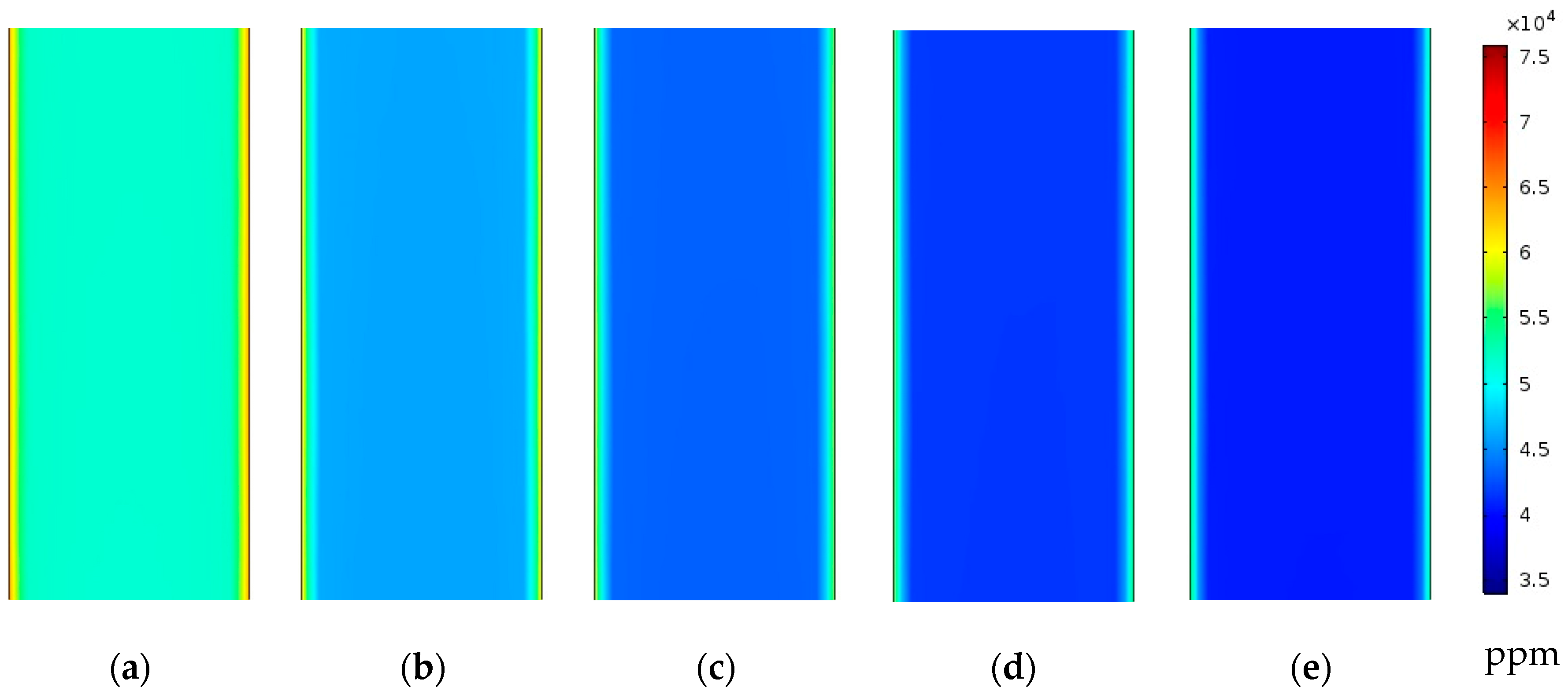
Figure 5.
Feed water salinity contours at middle of half section in the feed channel of desalination unit with single straight fiber at ; (a) , (b) , (c) , (d) , and (e) .
Figure 5.
Feed water salinity contours at middle of half section in the feed channel of desalination unit with single straight fiber at ; (a) , (b) , (c) , (d) , and (e) .
Figure 6.
Feed water temperature contours at cross section at middle of fiber length of desalination unit with single straight fiber at ; (a) , (b) , (c) , (d) , and (e) .
Figure 6.
Feed water temperature contours at cross section at middle of fiber length of desalination unit with single straight fiber at ; (a) , (b) , (c) , (d) , and (e) .
Figure 7.
Temperature contours at middle of section in desalination unit at with single fiber [(a) , (b) , (c) and (d) ], and double straight fibers [(e) , (f) , (g) and (h) ]. The arrows represent the axial velocity magnitudes relative to each other.
Figure 7.
Temperature contours at middle of section in desalination unit at with single fiber [(a) , (b) , (c) and (d) ], and double straight fibers [(e) , (f) , (g) and (h) ]. The arrows represent the axial velocity magnitudes relative to each other.
Figure 8.
Water gap temperature contours at middle of section at for desalination unit with single (a) straight fiber with (b) , (c) , (d) , (e) , and (f) turns of helical fibers and double (g) straight fibers with (h) , (i) , (j) , (k) , and (l) turns of helical fibers.
Figure 8.
Water gap temperature contours at middle of section at for desalination unit with single (a) straight fiber with (b) , (c) , (d) , (e) , and (f) turns of helical fibers and double (g) straight fibers with (h) , (i) , (j) , (k) , and (l) turns of helical fibers.
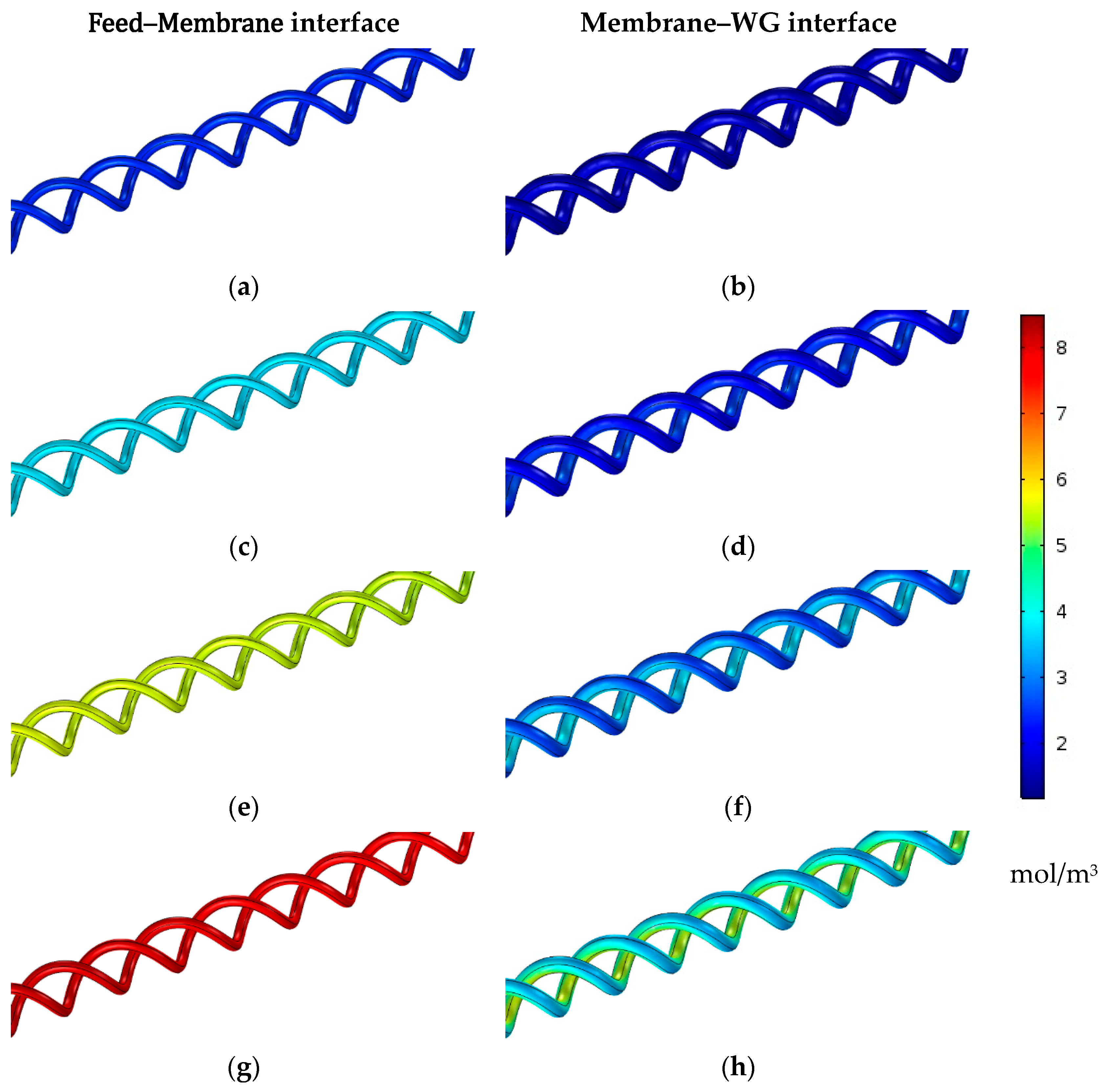
Figure 9.
Water vapor concentration contours on both HF membrane interfaces with turns of double helical fibers at . (a,b) , (c,d) , (e,f) , and (g,h) .
Figure 9.
Water vapor concentration contours on both HF membrane interfaces with turns of double helical fibers at . (a,b) , (c,d) , (e,f) , and (g,h) .
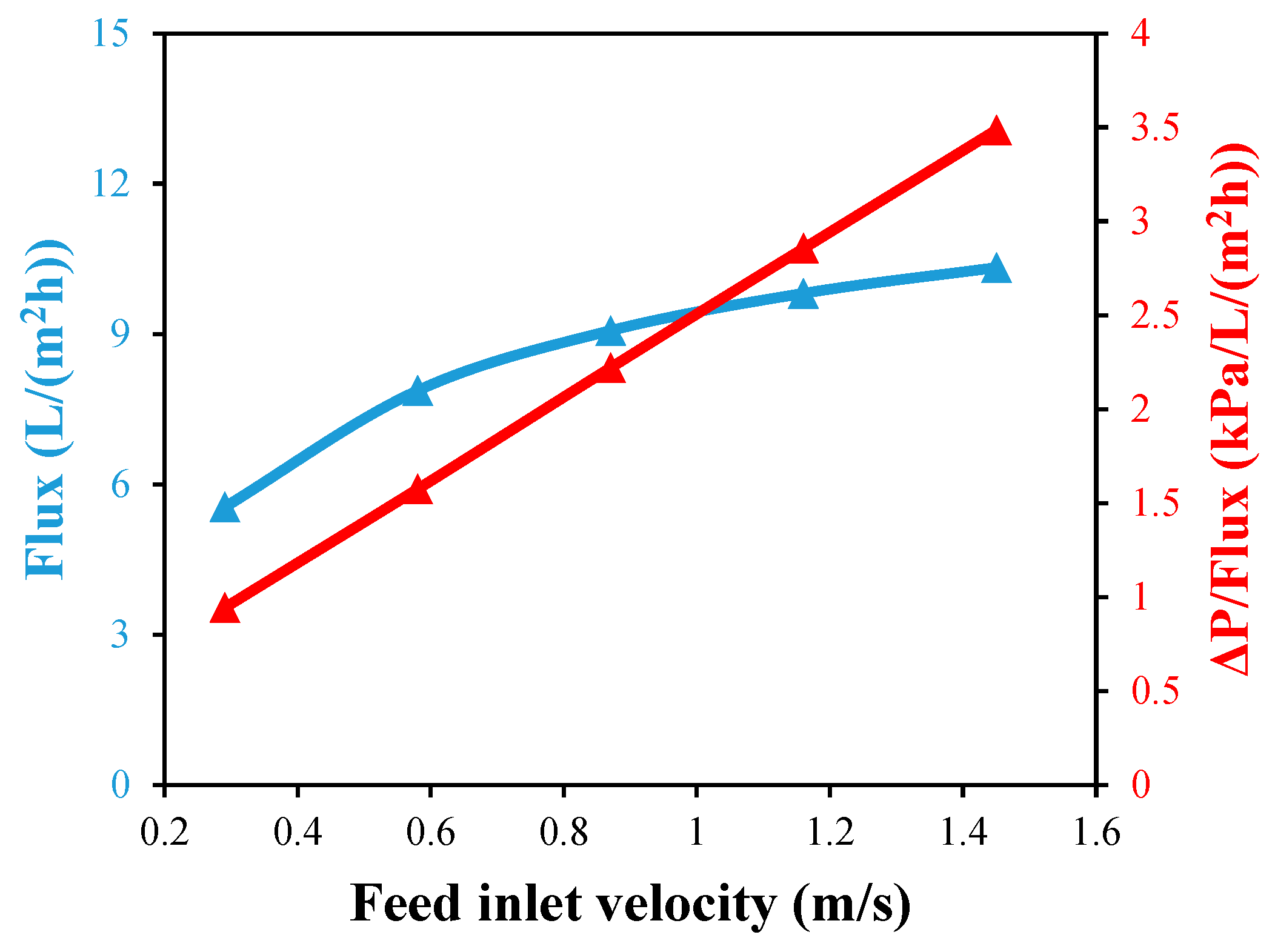
Figure 10.
Water output flux and pressure drop per unit flux against feed inlet velocity with single straight fiber module at and .
Figure 10.
Water output flux and pressure drop per unit flux against feed inlet velocity with single straight fiber module at and .
Figure 11.
Water output flux against number of HF helical turns at different coolant inlet velocities and for desalination units with (a) single helical fiber and (b) double helical fibers.
Figure 11.
Water output flux against number of HF helical turns at different coolant inlet velocities and for desalination units with (a) single helical fiber and (b) double helical fibers.
Figure 12.
Water output flux against coolant inlet velocity at for a desalination unit with turns of helical fiber; (a) single and (b) double.
Figure 12.
Water output flux against coolant inlet velocity at for a desalination unit with turns of helical fiber; (a) single and (b) double.
Figure 13.
Water output flux and specific productivity against number of HF helical turns for desalination unit with single fiber at ; (a) , (b) , (c) , and (d) .
Figure 13.
Water output flux and specific productivity against number of HF helical turns for desalination unit with single fiber at ; (a) , (b) , (c) , and (d) .
Figure 14.
Water output flux and specific productivity against number of HF helical turns for desalination unit with double fibers at ; (a) , (b) , (c) , and (d) .
Figure 14.
Water output flux and specific productivity against number of HF helical turns for desalination unit with double fibers at ; (a) , (b) , (c) , and (d) .
Figure 15.
STEC and %TER against number of HF helical turns for desalination unit with single fiber at ; (a) , (b) , (c) , and (d) .
Figure 15.
STEC and %TER against number of HF helical turns for desalination unit with single fiber at ; (a) , (b) , (c) , and (d) .
Figure 16.
STEC and %TER against number of HF helical turns for desalination unit with double fibers at ; (a) , (b) , (c) , and (d) .
Figure 16.
STEC and %TER against number of HF helical turns for desalination unit with double fibers at ; (a) , (b) , (c) , and (d) .
Figure 17.
The effect of multi-stages in series on the GOR and STEC of of single helical fiber desalination units at , and .
Figure 17.
The effect of multi-stages in series on the GOR and STEC of of single helical fiber desalination units at , and .
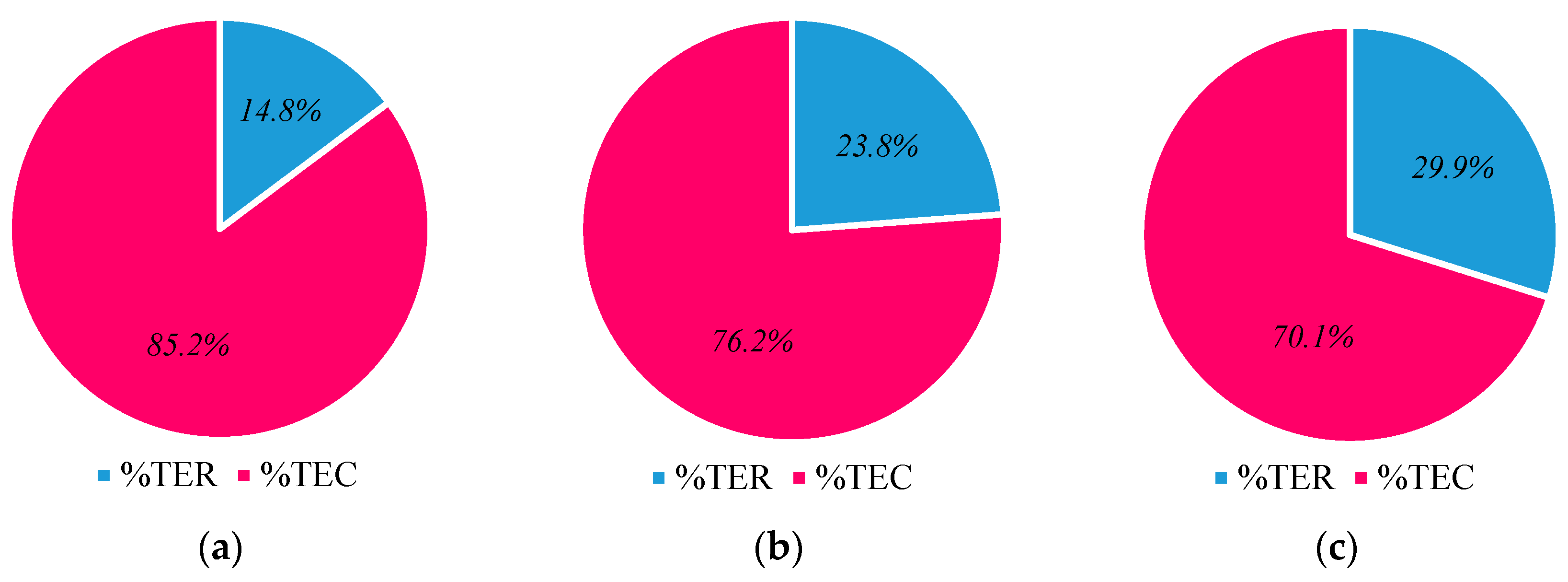
Figure 18.
Percentage of thermal energy recovered of (a) one, (b) two, and (c) three single helical fiber desalination units with 50 turns fitted in series at , and .
Figure 18.
Percentage of thermal energy recovered of (a) one, (b) two, and (c) three single helical fiber desalination units with 50 turns fitted in series at , and .
Table 1.
Geometrical characteristics and operational conditions of the simulated HF-WGMD unit.
Table 1.
Geometrical characteristics and operational conditions of the simulated HF-WGMD unit.
| Parameter | Symbol | Value | Unit |
|---|
| HF membrane inner diameter | | 0.8 | mm |
| HF membrane outer diameter | | 1.16 | mm |
| Cooling tube inner diameter | | 5 | mm |
| Cooling tube outer diameter | | 5.56 | mm |
| Cooling tube spacing | | 6.95 | mm |
| Module effective length | | 500 | mm |
| Feed inlet salinity | - | 35,000 | ppm |
| Water gap salinity | - | 0.0 | ppm |
| Coolant inlet temperature | | 20 | °C |
| Feed water thermal conductivity | | 0.64 | W/m K |
| Membrane thermal conductivity | | 0.07 | W/m K |
| Cooling tube thermal conductivity | | 0.445 | W/m K |
| Membrane porosity | | 82 | % |
| Membrane pore tortuosity | | 1.698 | - |
| Membrane pore diameter | | 0.16 | μm |
| Water vapor molar mass | | 18 | g/mol |
| Salt molar mass | | 58.4 | g/mol |
Table 2.
The external boundary conditions of the simulated desalination unit.
Table 2.
The external boundary conditions of the simulated desalination unit.
| Domain | Position | Boundary Conditions |
|---|
| Mass | Momentum | Energy |
|---|
| Feed channel | | | | |
| | | |
| HF membrane | | | - | |
| | - | |
| Water gap | | - | - | |
| - | - | |
| Cooling tube | | - | - | |
| - | - | |
| Cooling channel | | - | | |
| - | | |
| - | | |
| - | | |
Table 3.
Grid independence study on a case of single straight fiber with and .
Table 3.
Grid independence study on a case of single straight fiber with and .
| | Number of Grid Elements | Water Flux (L/(m2 h)) | %Variation in Water Flux | Feed Outlet Temperature (°C) | % Variation in Feed Outlet Temperature |
|---|
| Grid 1 | 1,203,853 | 8.83 | - | 59.131 | - |
| Grid 2 | 2,411,325 | 9.05 | 2.492 | 59.349 | 0.369 |
| Grid 3 | 5,168,202 | 9 | −0.552 | 59.438 | 0.15 |
Table 4.
Operational and geometrical parameters of experimental modules used in CFD model validation.
Table 4.
Operational and geometrical parameters of experimental modules used in CFD model validation.
| Reference | Experimental Module | Number of Fibers per Tube | Module Length (mm) | Feed Inlet Temperature (°C) | Feed Inlet Velocity
(m/s) |
|---|
| [28] | Module 1 | 1 | 350 | 40, 50, 60, and 70 | 0.69 |
| Module 2 | 2 |
| Module 3 | 3 |
| [14] | Variable feed inlet temperatures | 1 | 425 | 0.81 |
| Variable feed inlet velocities | 70 | 0.28, 0.4, 0.53, 0.69, and 0.81 |
Table 5.
Salinity and temperature at feed–membrane interface at fiber middle length of desalination unit with single straight fiber at different feed inlet velocities.
Table 5.
Salinity and temperature at feed–membrane interface at fiber middle length of desalination unit with single straight fiber at different feed inlet velocities.
| | (m/s) |
|---|
| 0.29 | 0.58 | 0.87 | 1.16 | 1.45 |
|---|
| Salinity (ppm) | 65,401 | 62,941 | 61,552 | 60,269 | 58,945 |
| Temperature (°C) | 51.9 | 59 | 61.8 | 63.3 | 64.2 |
Table 6.
Water gap average temperature at different cross sections along desalination unit with single and double straight fibers at different coolant inlet velocities.
Table 6.
Water gap average temperature at different cross sections along desalination unit with single and double straight fibers at different coolant inlet velocities.
| | | | |
|---|
| WG Average Temperature (°C) |
|---|
| Single | 61.3 | 56.4 | 48.2 |
| Double | 67.5 | 64.7 | 58.6 |
| Single | 44.6 | 41.6 | 37.7 |
| Double | 55.2 | 50.6 | 46.3 |
| Single | 36.1 | 35.2 | 33.5 |
| Double | 44.6 | 41.4 | 39.7 |
| Single | 33.4 | 33.2 | 32.2 |
| Double | 40.4 | 38.1 | 37.5 |
Table 7.
Water gap average temperatures with single and double fibers.
Table 7.
Water gap average temperatures with single and double fibers.
| | WG Average Temperature (°C) |
|---|
| Straight | Turns | Turns | Turns | Turns | Turns |
|---|
| Single | 31.4 | 30 | 30.5 | 31.2 | 32 | 32.9 |
| Double | 38.2 | 38.4 | 39.2 | 40.4 | 41.5 | 42.9 |
Table 8.
Average water vapor concentration differences across the HF membrane with single and double fibers.
Table 8.
Average water vapor concentration differences across the HF membrane with single and double fibers.
| | Average Concentration Difference (mol/m3) |
|---|
| Straight | Turns | Turns | Turns | Turns | Turns |
|---|
| Single | 4.116 | 4.435 | 4.51 | 4.439 | 4.293 | 4.206 |
| Double | 3.792 | 4.069 | 4.116 | 4.009 | 3.837 | 3.709 |
Table 9.
Water vapor average concentration with turns of double helical fibers.
Table 9.
Water vapor average concentration with turns of double helical fibers.
| | Feed Inlet Temperature (°C) |
|---|
| 40 | 50 | 60 | 70 |
|---|
| Feed–membrane interface | 2.445 | 3.765 | 5.612 | 8.122 |
| Membrane–WG interface | 1.682 | 2.28 | 3.147 | 4.413 |
| Concentration difference | 0.763 | 1.485 | 2.465 | 3.709 |


 ,
, 


