

The Role of the Morphological Characterization of Multilayer Hydrophobized Ceramic Membranes on the Prediction of Sweeping Gas Membrane Distillation Performances

Abstract
:1. Introduction
2. Materials and Methods
2.1. Membranes and Modules
2.2. Experimental Set-Up and Procedures
3. SGMD of NaCl-Water Solutions across Capillary Bundles: Model Equations
- Steady-state conditions;
- Total NaCl rejection: the membrane is a perfect barrier and thus only water permeates;
- Gas phase behaves as an ideal gas mixture;
- No heat loss in the module (well-insulated module);
- Parallel flow of liquid and gas streams within the module.
3.1. Local Model: Heat and Mass Transfer across The Membrane
3.2. Module Simulation
4. Results and Discussion
5. Conclusions
Author Contributions
Funding
Institutional Review Board Statement
Data Availability Statement
Conflicts of Interest
List of Symbols
| Latin Letters | SI Units | |
| Inner surface Area | [m2] | |
| Molar, mass, heat capacity at constant pressure | [J mol−1 K−1], [J kg−1 K−1] | |
| Inner diameter of a fiber | [m] | |
| Outer diameter of a fiber | [m] | |
| Logarithmic mean diameter of the membrane | [m] | |
| Logarithmic mean diameter of the membrane layer j | [m] | |
| Shell diameter | [m] | |
| Pore diameter of the membrane layer j | [m] | |
| Mean pore diameter of the membrane | [m] | |
| Knudsen diffusion coefficient of water | [m2 s−1] | |
| Molecular diffusion coefficient of water in gas | [m2 s−1] | |
| Equivalent diffusion coefficient of water | [m2 s−1] | |
| D | Molecular diffusion coefficient | [m2 s−1] |
| f | Fanning factor | [dimensionless] |
| Inlet stream of gas | ||
| Outlet stream of gas | ||
| Graetz number for heat, mass transfer | [dimensionless] | |
| h | Convective heat transfer coefficient | [W m−2 K−1] |
| Mass flux of water across the membrane (defined in Equation (2)) | [kg m−2 s−1) | |
| Mass transfer coefficient of water | [m s−1] | |
| Mass transfer coefficient of salt in liquid | [m s−1] | |
| Thermal conductivity coefficient | [W m−1 K−1] | |
| Pseudo-thermal conductivity of the membrane (defined in Equation (9a)) | [W m−2 K−1] | |
| Effective length of membrane module (Figure 1c) | [m] | |
| Total length of membrane module | [m] | |
| Inlet stream of liquid | ||
| Outlet stream of liquid | ||
| Mass of water in the liquid side | [kg] | |
| Total mass of solution in the liquid side | [kg] | |
| M | Molar mass | [kg mol−1] |
| Molar flow rate | [mol s−1] | |
| Transmembrane Molar flow rate of water per unit length per fiber | [mol m−1 s−1] | |
| Number of fibers | [dimensionless] | |
| Nu | Nusselt number | [dimensionless] |
| P | Pressure | [Pa] |
| Pr | Prandtl number | [dimensionless] |
| Vapor pressure of water | [Pa] | |
| Heat flow rate per unit length per fiber in the liquid thermal boundary layer | [W m−1] | |
| Net transmembrane heat flow rate per unit length per fiber | [W m−1] | |
| Re | Reynolds number | [dimensionless] |
| Universal gas constant | [J mol−1 K−1] | |
| Salinity of NaCl solution | [g NaCl kg−1 Solution] | |
| Sc | Schmidt number | [dimensionless] |
| Sh | Sherwood number | [dimensionless] |
| T | Temperature | [K] |
| Liquid velocity in lumen-side (defined in Equation (15)) | [m s−1] | |
| Gas interstitial velocity in shell-side (defined in Equation (21)) | [m s−1] | |
| x | Mole fraction in liquid phase | [dimensionless] |
| y | Mole fraction in gas phase | [dimensionless] |
| z | Axial coordinate in membrane module | [m] |
| Greek Letters | SI Units | |
| Activity coefficient of water at liquid/membrane interface | [dimensionless] | |
| Thickness | [m] | |
| Porosity-tortuosity ratio of the membrane layer j | [dimensionless] | |
| Mean porosity-tortuosity ratio of the membrane | [dimensionless] | |
| Packing factor of the membrane module | [dimensionless] | |
| Dynamic viscosity | [Pa s] | |
| Molar latent heat of vaporization | [J mol−1] | |
| Density | [kg m−3] | |
| Superscripts and Subscripts | ||
| a | Air | |
| G | Gas side | |
| Gb | At gas bulk | |
| Gm | At gas/membrane interface | |
| IN | Inlet section | |
| j | Layer j (j = S for support, j = 1 for layer1, j = 2 for layer 2, j = 3 for layer 3) | |
| L | Liquid side | |
| Lb | At liquid bulk | |
| Lm | At liquid/membrane interface | |
| s | Salt | |
| solid | Solid portion of the membrane | |
| w | Water | |
Appendix A. Mass and Heat Transfer Correlations

| Side | Correlation | Validity Range | Reference |
|---|---|---|---|
| Tube | (A.1) | [44,45] | |
| (A.2) | [46,47] | ||
| Shell (parallel flow) | (A.3) (in inches) | [44] |
| Heat Transfer | Mass Transfer |
|---|---|
Appendix B. Relevant Chemical-Physical Properties
References
- Ahmed, F.E.; Khalil, A.; Hilal, N. Emerging Desalination Technologies: Current Status, Challenges and Future Trends. Desalination 2021, 517, 115183. [Google Scholar] [CrossRef]
- Alkhudhiri, A.; Darwish, N.; Hilal, N. Membrane Distillation: A Comprehensive Review. Desalination 2012, 287, 2–18. [Google Scholar] [CrossRef]
- Drioli, E.; Criscuoli, A.; Curcio, E. Membrane Contactors: Fundamentals, Applications and Potentialities; Elsevier: Amsterdam, The Netherlands, 2006. [Google Scholar]
- Khayet, M.; Matsuura, T. Membrane Distillation-Principles and Applications; Elsevier: Amsterdam, The Netherlands, 2011. [Google Scholar]
- Qasim, M.; Samad, I.U.; Darwish, N.A.; Hilal, N. Comprehensive Review of Membrane Design and Synthesis for Membrane Distillation. Desalination 2021, 518, 115168. [Google Scholar] [CrossRef]
- Ismail, M.S.; Mohamed, A.M.; Poggio, D.; Walker, M.; Pourkashanian, M. Modelling Mass Transport within the Membrane of Direct Contact Membrane Distillation Modules Used for Desalination and Wastewater Treatment: Scrutinising Assumptions. J. Water Process Eng. 2022, 45, 102460. [Google Scholar] [CrossRef]
- Alsalhy, Q.F.; Ibrahim, S.S.; Hashim, F.A. Experimental and Theoretical Investigation of Air Gap Membrane Distillation Process for Water Desalination. Chem. Eng. Res. Des. 2018, 130, 95–108. [Google Scholar] [CrossRef]
- Kebria, M.R.S.; Rahimpour, A.; Bakeri, G.; Abedini, R. Experimental and Theoretical Investigation of Thin ZIF-8/Chitosan Coated Layer on Air Gap Membrane Distillation Performance of PVDF Membrane. Desalination 2019, 450, 21–32. [Google Scholar] [CrossRef]
- Zhang, H.; Li, B.; Sun, D.; Miao, X.; Gu, Y. SiO2-PDMS-PVDF Hollow Fiber Membrane with High Flux for Vacuum Membrane Distillation. Desalination 2018, 429, 33–43. [Google Scholar] [CrossRef]
- Choudhury, M.R.; Anwar, N.; Jassby, D.; Rahaman, M.S. Fouling and Wetting in the Membrane Distillation Driven Wastewater Reclamation Process—A Review. Adv. Colloid. Interface Sci. 2019, 269, 370–399. [Google Scholar] [CrossRef]
- Wei, C.C.; Li, K. Preparation and Characterization of a Robust and Hydrophobic Ceramic Membrane via an Improved Surface Grafting Technique. Ind. Eng. Chem. Res. 2009, 48, 3446–3452. [Google Scholar] [CrossRef]
- Kujawa, J.; Kujawski, W.; Koter, S.; Jarzynka, K.; Rozicka, A.; Bajda, K.; Cerneaux, S.; Persin, M.; Larbot, A. Membrane Distillation Properties of TiO2 Ceramic Membranes Modified by Perfluoroalkylsilanes. Desalin. Water Treat. 2013, 51, 1352–1361. [Google Scholar] [CrossRef]
- Richter, H.; Kaemnitz, S.; Gruetzner, J.; Martin, D.; Voigt, I. Carbon Membrane, Process for the Manufacture of Carbon Membranes and Use Thereof. U.S. Patent US2016/0175767 A1, 23 June 2016. [Google Scholar]
- García-Fernández, L.; Wang, B.; García-Payo, M.C.; Li, K.; Khayet, M. Morphological Design of Alumina Hollow Fiber Membranes for Desalination by Air Gap Membrane Distillation. Desalination 2017, 420, 226–240. [Google Scholar] [CrossRef]
- Fan, Y.; Chen, S.; Zhao, H.; Liu, Y. Distillation Membrane Constructed by TiO2 Nanofiber Followed by Fluorination for Excellent Water Desalination Performance. Desalination 2017, 405, 51–58. [Google Scholar] [CrossRef]
- Picard, C.; Larbot, A.; Tronel-Peyroz, E.; Berjoan, R. Characterisation of Hydrophilic Ceramic Membranes Modified by Fluoroalkylsilanes into Hydrophobic Membranes. Solid State Sci. 2004, 6, 605–612. [Google Scholar] [CrossRef]
- Koonaphapdeelert, S.; Li, K. Preparation and Characterization of Hydrophobic Ceramic Hollow Fibre Membrane. J. Memb. Sci. 2007, 291, 70–76. [Google Scholar] [CrossRef]
- Krajewski, S.R.; Kujawski, W.; Bukowska, M.; Picard, C.; Larbot, A. Application of Fluoroalkylsilanes (FAS) Grafted Ceramic Membranes in Membrane Distillation Process of NaCl Solutions. J. Memb. Sci. 2006, 281, 253–259. [Google Scholar] [CrossRef]
- Krajewski, S.R.; Kujawski, W.; Dijoux, F.; Picard, C.; Larbot, A. Grafting of ZrO2 Powder and ZrO2 Membrane by Fluoroalkylsilanes. Colloids Surf. A Physicochem. Eng. Asp. 2004, 243, 43–47. [Google Scholar] [CrossRef]
- Varela-Corredor, F.; Bandini, S. Advances in Water Breakthrough Measurement at High Temperature in Macroporous Hydrophobic Ceramic/Polymeric Membranes. J. Memb. Sci. 2018, 565, 72–84. [Google Scholar] [CrossRef]
- Varela-Corredor, F.; Bandini, S. Testing the Applicability Limits of a Membrane Distillation Process with Ceramic Hydrophobized Membranes: The Critical Wetting Temperature. Sep. Purif. Technol. 2020, 250, 117205. [Google Scholar] [CrossRef]
- Claramunt, S.; Völker, F.; Gerhards, U.; Kraut, M.; Dittmeyer, R. Membranes for the Gas/Liquid Phase Separation at Elevated Temperatures: Characterization of the Liquid Entry Pressure. Membranes 2021, 11, 907. [Google Scholar] [CrossRef]
- Fawzy, M.K.; Varela-Corredor, F.; Bandini, S. On the Morphological Characterization Procedures of Multilayer Hydrophobic Ceramic Membranes for Membrane Distillation Operations. Membranes 2019, 9, 125. [Google Scholar] [CrossRef] [Green Version]
- Kong, J.; Li, K. An Improved Gas Permeation Method for Characterising and Predicting the Performance of Microporous Asymmetric Hollow Fibre Membranes Used in Gas Absorption. J. Memb. Sci. 2001, 182, 271–281. [Google Scholar] [CrossRef]
- Karanikola, V.; Corral, A.F.; Jiang, H.; Eduardo Sáez, A.; Ela, W.P.; Arnold, R.G. Sweeping Gas Membrane Distillation: Numerical Simulation of Mass and Heat Transfer in a Hollow Fiber Membrane Module. J. Memb. Sci. 2015, 483, 15–24. [Google Scholar] [CrossRef]
- Elsheniti, M.B.; Elbessomy, M.O.; Wagdy, K.; Elsamni, O.A.; Elewa, M.M. Augmenting the Distillate Water Flux of Sweeping Gas Membrane Distillation Using Turbulators: A Numerical Investigation. Case Stud. Therm. Eng. 2021, 26, 101180. [Google Scholar] [CrossRef]
- Weyd, M.; Richter, H.; Puhlfürß, P.; Voigt, I.; Hamel, C.; Seidel-Morgenstern, A. Transport of Binary Water-Ethanol Mixtures through a Multilayer Hydrophobic Zeolite Membrane. J. Memb. Sci. 2008, 307, 239–248. [Google Scholar] [CrossRef]
- Voigt, I.; Fischer, G.; Puhlfürß, P.; Schleifenheimer, M.; Stahn, M. TiO2-NF-Membranes on Capillary Supports. Sep. Purif. Technol. 2003, 32, 87–91. [Google Scholar] [CrossRef]
- Richter, H.; Voigt, I.; Fischer, G.; Puhlfürß, P. Preparation of Zeolite Membranes on the Inner Surface of Ceramic Tubes and Capillaries. Sep. Purif. Technol. 2003, 32, 133–138. [Google Scholar] [CrossRef]
- Voigt, I.; Dudziak, G.; Hoyer, T.; Nickel, A.; Puhlfuerss, P. Membrana Ceramica DeNanofiltracao Para AUtilizacao Em Solvents Organicos e Processo Para a Sua Preparacao. PT Patent PT 1603663 E, 25 February 2004. [Google Scholar]
- Pashkova, A.; Dittmeyer, R.; Kaltenborn, N.; Richter, H. Experimental Study of Porous Tubular Catalytic Membranes for Direct Synthesis of Hydrogen Peroxide. Chem. Eng. J. 2010, 165, 924–933. [Google Scholar] [CrossRef]
- Zeidler, S.; Puhlfürß, P.; Kätzel, U.; Voigt, I. Preparation and Characterization of New Low MWCO Ceramic Nanofiltration Membranes for Organic Solvents. J. Memb. Sci. 2014, 470, 421–430. [Google Scholar] [CrossRef]
- Bird, R.B.; Stewart, W.E.; Lightfoot, E.N. Transport Phenomena, 2nd ed.; John Wiley & Sons: Hoboken, NJ, USA, 2002. [Google Scholar]
- Scott, D.S.; Dullien, F.A.L. The Flow of Rarefied Gases. AIChE J. 1962, 8, 293–297. [Google Scholar] [CrossRef]
- Gostoli, C.; Gatta, A. Mass Transfer in a Hollow Fiber Dialyzer. J. Memb. Sci. 1980, 6, 133–148. [Google Scholar] [CrossRef]
- Alqsair, U.F.; Alshwairekh, A.M.; Alwatban, A.M.; Oztekin, A. Computational Study of Sweeping Gas Membrane Distillation Process–Flux Performance and Polarization Characteristics. Desalination 2020, 485, 114444. [Google Scholar] [CrossRef]
- Li, G.; Lu, L. Modeling and Performance Analysis of a Fully Solar-Powered Stand-Alone Sweeping Gas Membrane Distillation Desalination System for Island and Coastal Households. Energy Convers. Manag. 2020, 205, 112375. [Google Scholar] [CrossRef]
- Chen, Q.; Muhammad, B.; Akhtar, F.H.; Ybyraiymkul, D.; Muhammad, W.S.; Li, Y.; Ng, K.C. Thermo-Economic Analysis and Optimization of a Vacuum Multi-Effect Membrane Distillation System. Desalination 2020, 483, 114413. [Google Scholar] [CrossRef]
- Guan, G.; Yang, X.; Wang, R.; Field, R.; Fane, A.G. Evaluation of Hollow Fiber-Based Direct Contact and Vacuum Membrane Distillation Systems Using Aspen Process Simulation. J. Memb. Sci. 2014, 464, 127–139. [Google Scholar] [CrossRef]
- Aboulkasem, A.; Hassan, M.; Ibrahim, A.; El-Shamarka, S. Numerical Study of Transfer Processes in Sweeping Gas Membrane Water Distillation. Int. Conf. Appl. Mech. Mech. Eng. 2016, 17, 1–18. [Google Scholar] [CrossRef]
- Li, L.; Wang, J.W.; Zhong, H.; Hao, L.Y.; Abadikhah, H.; Xu, X.; Chen, C.S.S. Agathopoulos, Novel A-Si3N4 planar nanowire superhydrophobic membrane prepared through in-situ nitridation of silicon for membrane distillation. J. Memb. Sci. 2017, 543, 98–105. [Google Scholar] [CrossRef]
- Yang, M.Y.; Wang, J.W.; Li, L.; Dong, B.B.; Xin, X.S. Agathopoulos, Fabrication of low thermal conductivity yttrium silicate ceramic flat membrane for membrane distillation. J. Eur. Ceram. Soc. 2019, 39, 442–448. [Google Scholar] [CrossRef]
- Gu, J.; Ren, C.; Zong, X.; Chen, C.; Winnubst, L. Preparation of alumina membranes comprising a thin separation layer and a support with straight open pores for water desalination. Ceram. Int. 2016, 42, 12427–12434. [Google Scholar] [CrossRef]
- Knudsen, J.G.; Katz, D.L. Fluid Dynamics and Heat Transfer Part II, 1st ed.; McGRAW-Hill Inc.: New York, NY, USA, 1958. [Google Scholar]
- Green, D.W.; Perry, R.H. Perry’s Chemical Engineers’ Handbook, 8th ed.; McGraw-Hill Professional Publishing: New York, NY, USA, 2007. [Google Scholar]
- Perry, R.H.; Green, D.W. Perry’s Chemical Engineers’ Handbook, 6th ed.; McGraw-Hill Professional Publishing: New York, NY, USA, 1984. [Google Scholar]
- Leyuan, Y.; Dong, L. Single-Phase Thermal Transport of Nanofluids in a Mini Channel. J. Heat Transf. 2009, 133, 1477–1485. [Google Scholar] [CrossRef]
- Sharqawy, M.H.; Lienhard, V.J.H.; Zubair, S.M. Thermophysical Properties of Seawater: A Review of Existing Correlations and Data. Desalination Water Treat 2010, 16, 354–380. [Google Scholar] [CrossRef]
- Poling, B.E.; Prausnitz, J.M.; O’connell, J.P.; York, N.; San, C.; Lisbon, F.; Madrid, L.; City, M.; Delhi, M.N.; Juan, S. The Properties of Gases and Liquids, 5th ed.; McGRAW-Hill: New York, NY, USA, 2001. [Google Scholar] [CrossRef]
- Robinson, R.A.; Stokes, R.H. Electrolyte Solutions, 2nd ed.; Butterworth & CO., Ltd.: London, UK, 1970. [Google Scholar]
- Shackelford, J.F.; Alexander, W. CRC Materials Science and Engineering Handbook, 3rd ed; CRC Press: Boca Raton, FL, USA, 2000. [Google Scholar]


| Code | dIN (mm) | dOUT (mm) | Nf (fibers) | Ltot (cm) | dS (cm) | Leff (cm) | AIN (cm2) | LEPmin (at T) (bar) |
|---|---|---|---|---|---|---|---|---|
| B2754 | 1.56 | 3.20 | 37 | 20 | 3.60 | 13 | 363 | 4.2 (25 °C) |
| B2755 | 1.56 | 3.20 | 37 | 20 | 3.60 | 13 | 363 | 4 (25 °C) |
| B2756 | 1.56 | 3.20 | 37 | 20 | 3.60 | 13 | 363 | 6.2 (25 °C) |
| B2888 | 1.9 | 3.54 | 37 | 20 | 3.60 | 13 | 442 | 0.30–0.39 (130 °C) § |
| B2758 | 1.9 | 3.20 | 22 | 20 | 2.50 | 17 | 263 | 6.9 (25 °C) § |
| Layer 3 | Layer 2 | Layer 1 | Support | |||||||||
|---|---|---|---|---|---|---|---|---|---|---|---|---|
| Code | dp (nm) | (ε/τ) | δ (µm) | dp (nm) | (ε/τ) | δ (µm) | dp (nm) | (ε/τ) | δ (µm) | dp (nm) | (ε/τ) | δ (µm) |
| B2754 | 548 | 0.0029 | 10 | 250 | 0.34 | 30 | 800 | 0.20 | 30 | 4500 | 0.11 | 750 |
| B2755 | 534 | 0.0032 | 10 | 250 | 0.34 | 30 | 800 | 0.20 | 30 | 4500 | 0.11 | 750 |
| B2756 | 435 | 0.0044 | 10 | 250 | 0.34 | 30 | 800 | 0.20 | 30 | 4500 | 0.11 | 750 |
| B2888 | 328 | 0.0069 | 10 | 250 | 0.34 | 30 | 800 | 0.20 | 30 | 4500 | 0.11 | 750 |
| B2758 | 68 | 0.084 | 10 | 250 | 0.34 | 30 | 800 | 0.20 | 30 | 4500 | 0.11 | 580 |
| Average Values | ||
|---|---|---|
| Code | dpm (nm) | (ε/τ) |
| B2754 | 468 | 0.27 |
| B2755 | 1232 | 0.053 |
| B2756 | 354 | 0.44 |
| B2888 | 337 | 0.38 |
| B2758 | 87 | 3.414 |
| Liquid Inlet to Tube-Side (Lin) | Gas Inlet to Shell-Side (Gin) | ||||||||||
|---|---|---|---|---|---|---|---|---|---|---|---|
| Trial | T2 (°C) | P3 (bar) | F3 (L/h) | SNaCl (g/kg) | vL,IN (m/s) | ΔP (mbar) | T1 (°C) | P1 (bar) | F0 (m3STP/h) | v0,G,IN (m/s) | Bundle |
| B | 61.5 | 4.95 | 100 | 18.79 | 0.39 | - | 43.0 | 4.10 | 5.15 | 0.56 | B2755 |
| C | 88.9 | 2.55 | 100 | 18.92 | 0.39 | - | 49.0 | 2.20 | 2.91 | 0.60 | B2755 |
| D | 90.9 | 2.60 | 100 | 19.68 | 0.39 | - | 61.0 | 2.25 | 2.70 | 0.57 | B2756 |
| E | 89.9 | 2.45 | 100 | 18.24 | 0.39 | - | 51.5 | 1.90 | 1.87 | 0.45 | B2754 |
| F | 89.6 | 2.30 | 100 | 18.31 | 0.39 | - | 55.5 | 1.90 | 1.82 | 0.44 | B2754 |
| H | 64.6 | 3.34 | 100 | 19.50 | 0.45 | 170 | 41.7 | 4.05 | 1.71 | 0.58 | B2758 |
| I | 89.7 | 3.98 | 100 | 19.67 | 0.45 | 250 | 56.1 | 3.95 | 0.24 | 0.63 | B2758 |
| J | 64.1 | 2.90 | 100 | 19.82 | 0.45 | 200 | 43.1 | 2.70 | 1.51 | 0.58 | B2758 |
| K | 89.5 | 4.84 | 100 | 20.03 | 0.45 | 212 | 60.8 | 4.86 | 4.12 | 0.90 | B2758 |
| L | 40.9 | 2.30 | 100 | 18.58 | 0.45 | 310 | 39.3 | 2.13 | 2.05 | 0.98 | B2758 |
| M | 72.6 | 2.98 | 100 | 18.74 | 0.45 | 310 | 52.5 | 2.88 | 2.73 | 1.01 | B2758 |
| N | 50.3 | 5.13 | 104 | 18.90 | 0.46 | 325 | 44.5 | 5.00 | 4.64 | 0.96 | B2758 |
| O | 87.1 | 5.08 | 105 | 19.13 | 0.47 | 308 | 64.5 | 5.10 | 4.66 | 1.00 | B2758 |
| P | 110.3 | 5.33 | 103 | 19.58 | 0.46 | 329 | 69.8 | 5.23 | 4.87 | 1.03 | B2758 |
| Q | 110.2 | 5.25 | 100 | 19.93 | 0.45 | 290 | 69.3 | 5.10 | 4.76 | 1.03 | B2758 |
| R | 70.2 | 5.18 | 150 | 17.97 | 0.40 | 331 | 57.3 | 5.20 | 4.84 | 0.43 | B2888 |
| S | 89.3 | 5.13 | 150 | 18.75 | 0.40 | 296 | 61.5 | 5.25 | 4.87 | 0.44 | B2888 |
| T | 90.5 | 5.03 | 150 | 19.58 | 0.40 | 251 | 61.8 | 5.00 | 4.63 | 0.44 | B2888 |
| U | 91.10 | 5.05 | 150 | 19.95 | 0.40 | 264 | 62.0 | 5.08 | 4.66 | 0.43 | B2888 |
| Equation | Equation | |
|---|---|---|
| Total mass balance | (12) | |
| NaCl mass balance | (13) | |
| Heat balance | (14) | |
| Liquid velocity | (15) | |
| Pressure drop | (16) | |
| Boundary conditions |
| Equation | Equation | |
|---|---|---|
| Total mass balance | (17) | |
| Air mass balance | (18) | |
| Heat balance | (19) | |
| Ideal gas law | (20) | |
| Gas phase velocity | (21) | |
| Pressure drops (equivalent annulus model [35] | (22) | |
| Boundary conditions |
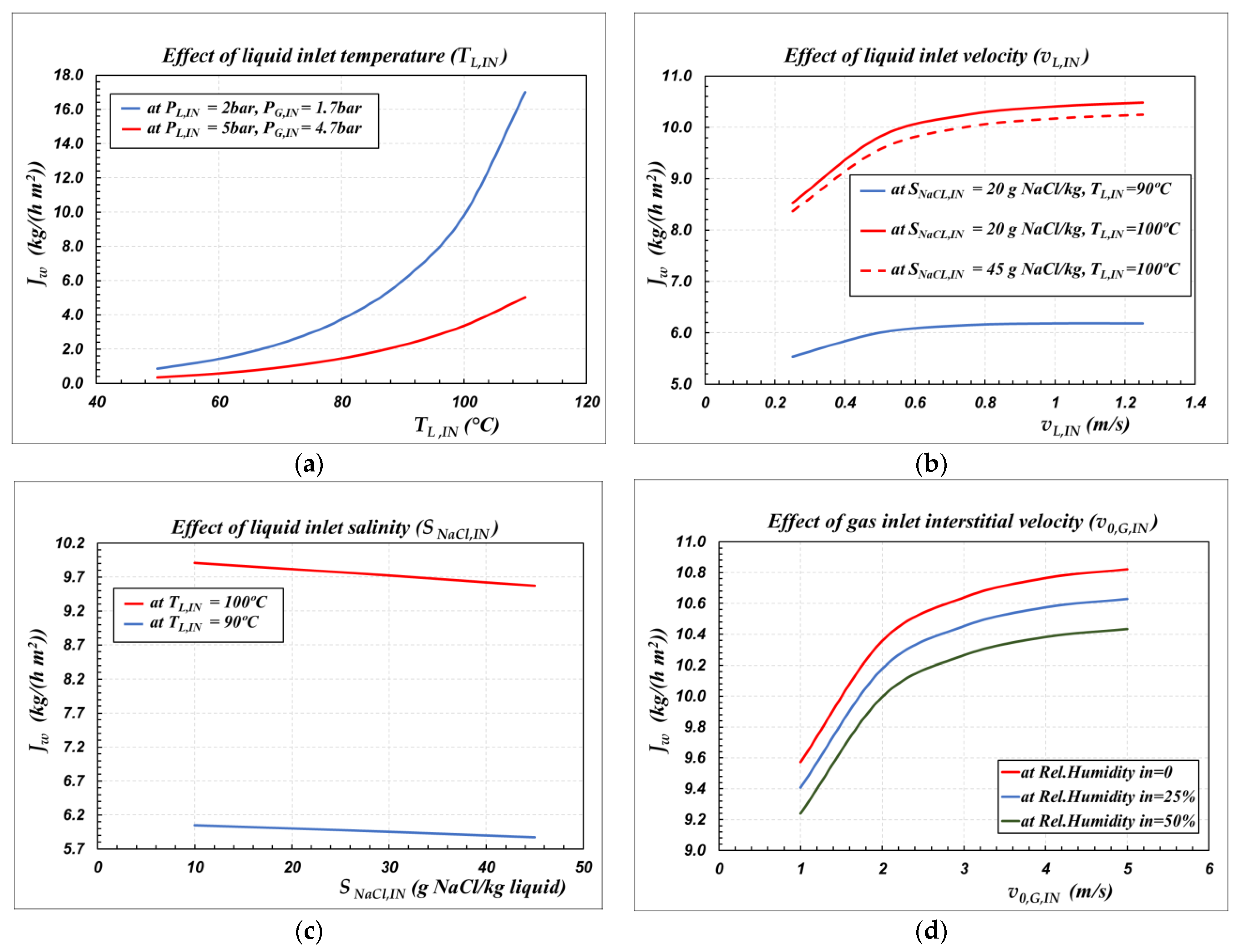
| Figure | 5a | 5b | 5c | 5d |
|---|---|---|---|---|
| TL,IN (°C) | * | * | * | 100 |
| PL,IN (bar) | * | 2 | 2 | 2 |
| SNaCl,IN (g/kg) | 20 | * | * | 45 |
| vL,IN (m/s) | 0.5 | * | 0.5 | 0.5 |
| TG,IN (°C) | 45 | 45 | 45 | 45 |
| PG,IN (bar) | * | 1.7 | 1.7 | 1.7 |
| Relative humidity of air (%) | 0 | 0 | 0 | * |
| v0,G,IN (m/s) | 1 | 1 | 1 | * |
Publisher’s Note: MDPI stays neutral with regard to jurisdictional claims in published maps and institutional affiliations. |
© 2022 by the authors. Licensee MDPI, Basel, Switzerland. This article is an open access article distributed under the terms and conditions of the Creative Commons Attribution (CC BY) license (https://creativecommons.org/licenses/by/4.0/).
Share and Cite
Fawzy, M.K.; Varela-Corredor, F.; Boi, C.; Bandini, S. The Role of the Morphological Characterization of Multilayer Hydrophobized Ceramic Membranes on the Prediction of Sweeping Gas Membrane Distillation Performances. Membranes 2022, 12, 939. https://doi.org/10.3390/membranes12100939
Fawzy MK, Varela-Corredor F, Boi C, Bandini S. The Role of the Morphological Characterization of Multilayer Hydrophobized Ceramic Membranes on the Prediction of Sweeping Gas Membrane Distillation Performances. Membranes. 2022; 12(10):939. https://doi.org/10.3390/membranes12100939
Chicago/Turabian StyleFawzy, Mohamed K., Felipe Varela-Corredor, Cristiana Boi, and Serena Bandini. 2022. "The Role of the Morphological Characterization of Multilayer Hydrophobized Ceramic Membranes on the Prediction of Sweeping Gas Membrane Distillation Performances" Membranes 12, no. 10: 939. https://doi.org/10.3390/membranes12100939