
Application of Soft-Clustering to Assess Consciousness in a CLIS Patient

Abstract
:1. Introduction
2. Materials and Methods
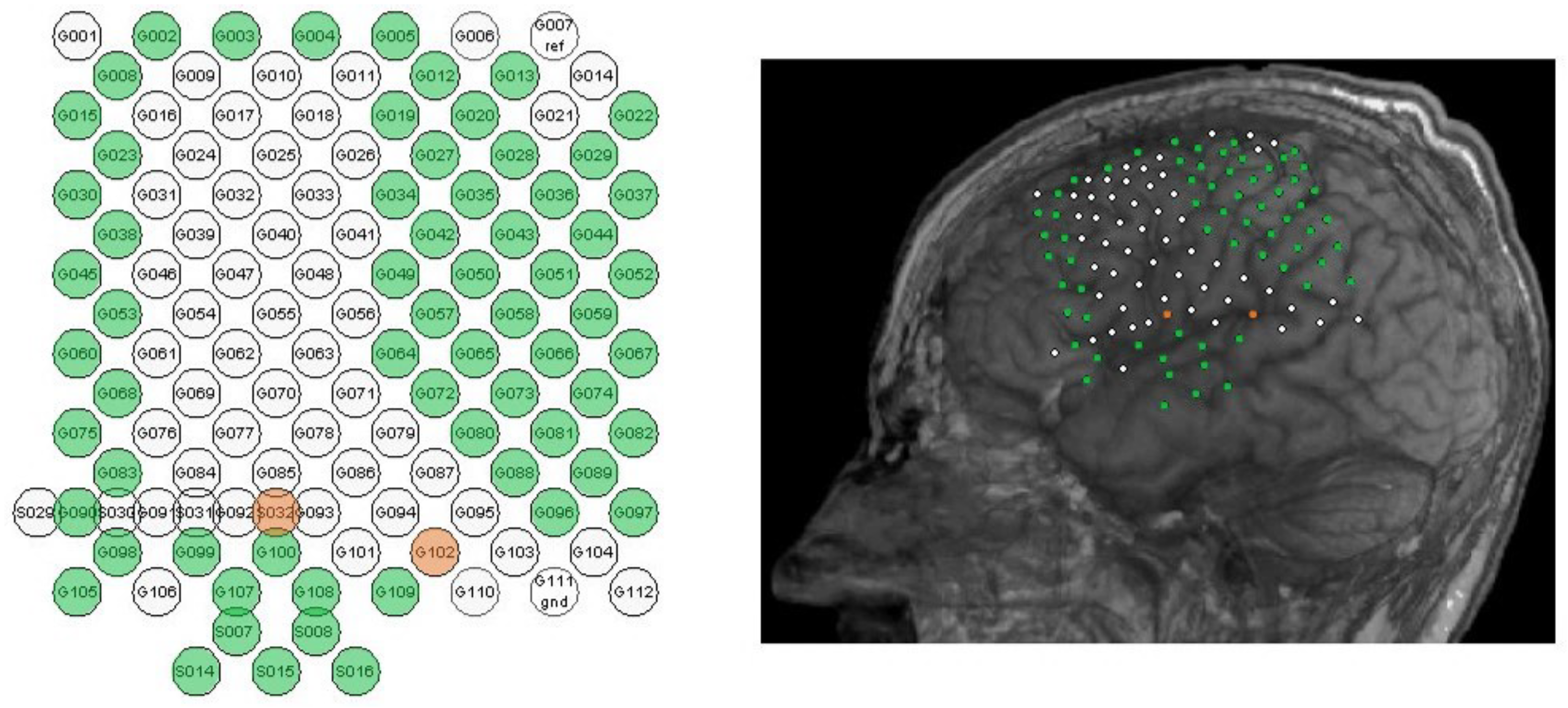
2.1. Patient Description
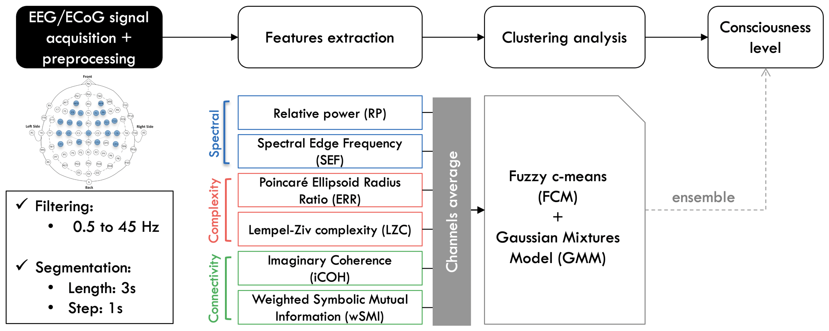
2.2. Methods Description
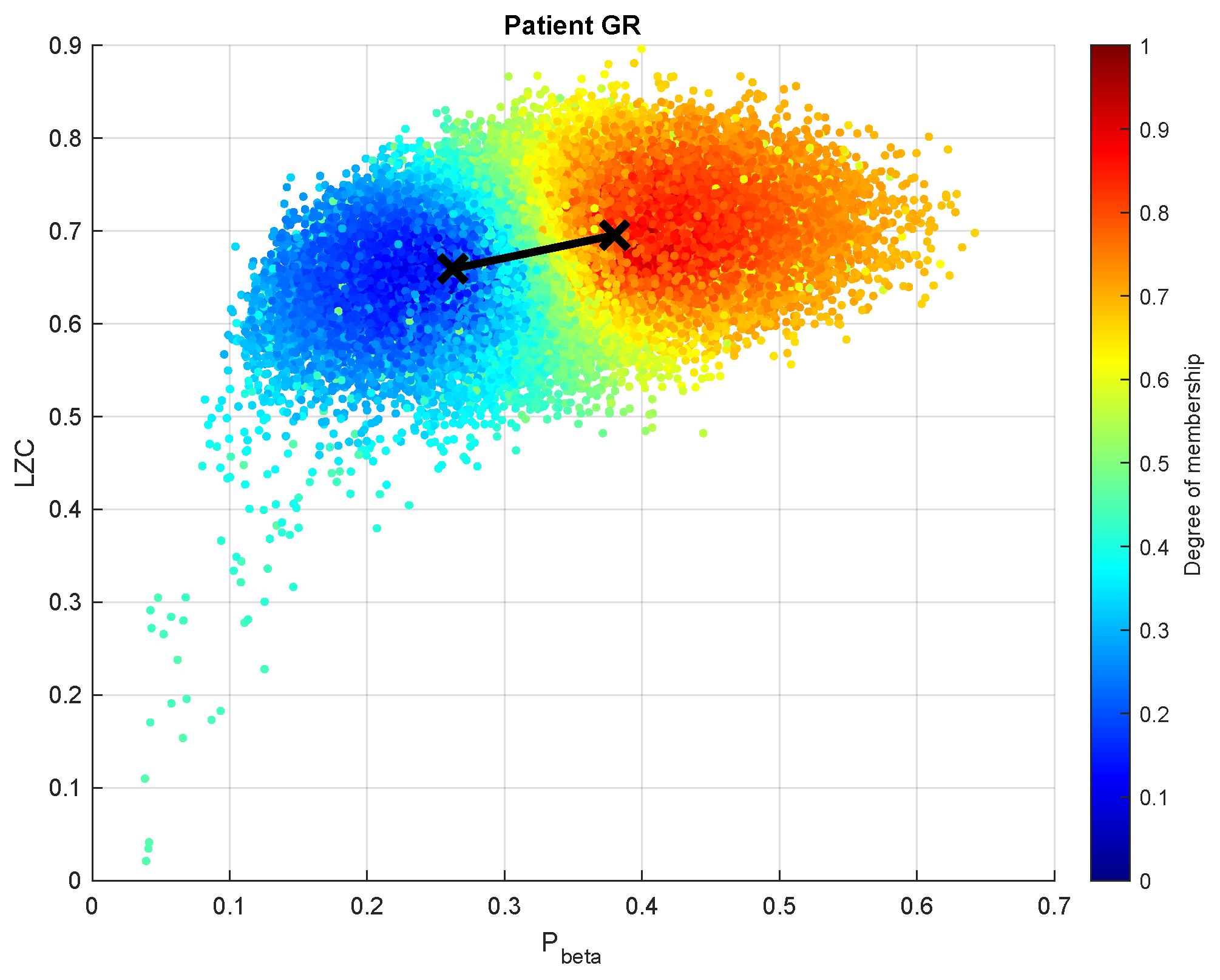
2.2.1. Features Computation
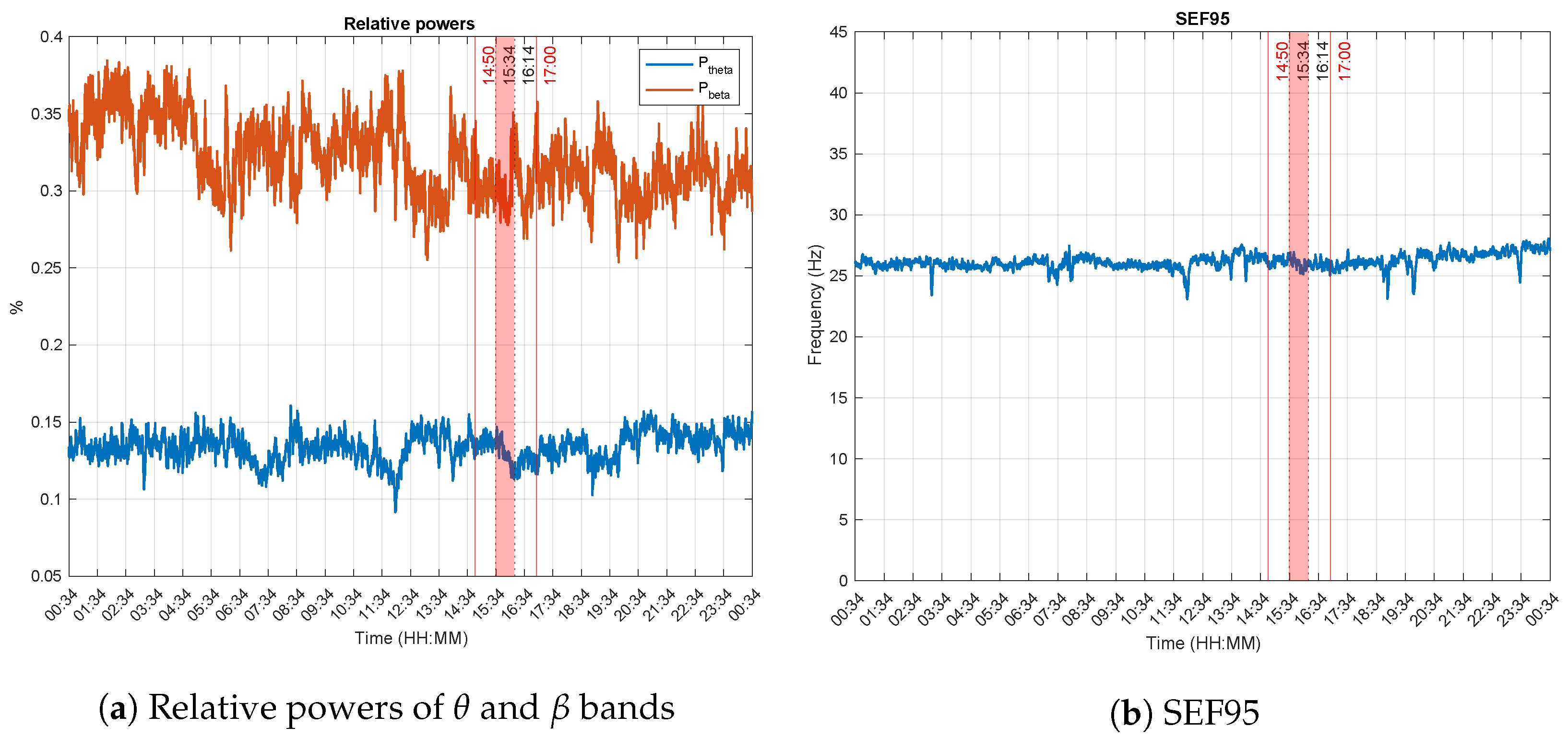
Spectral Features
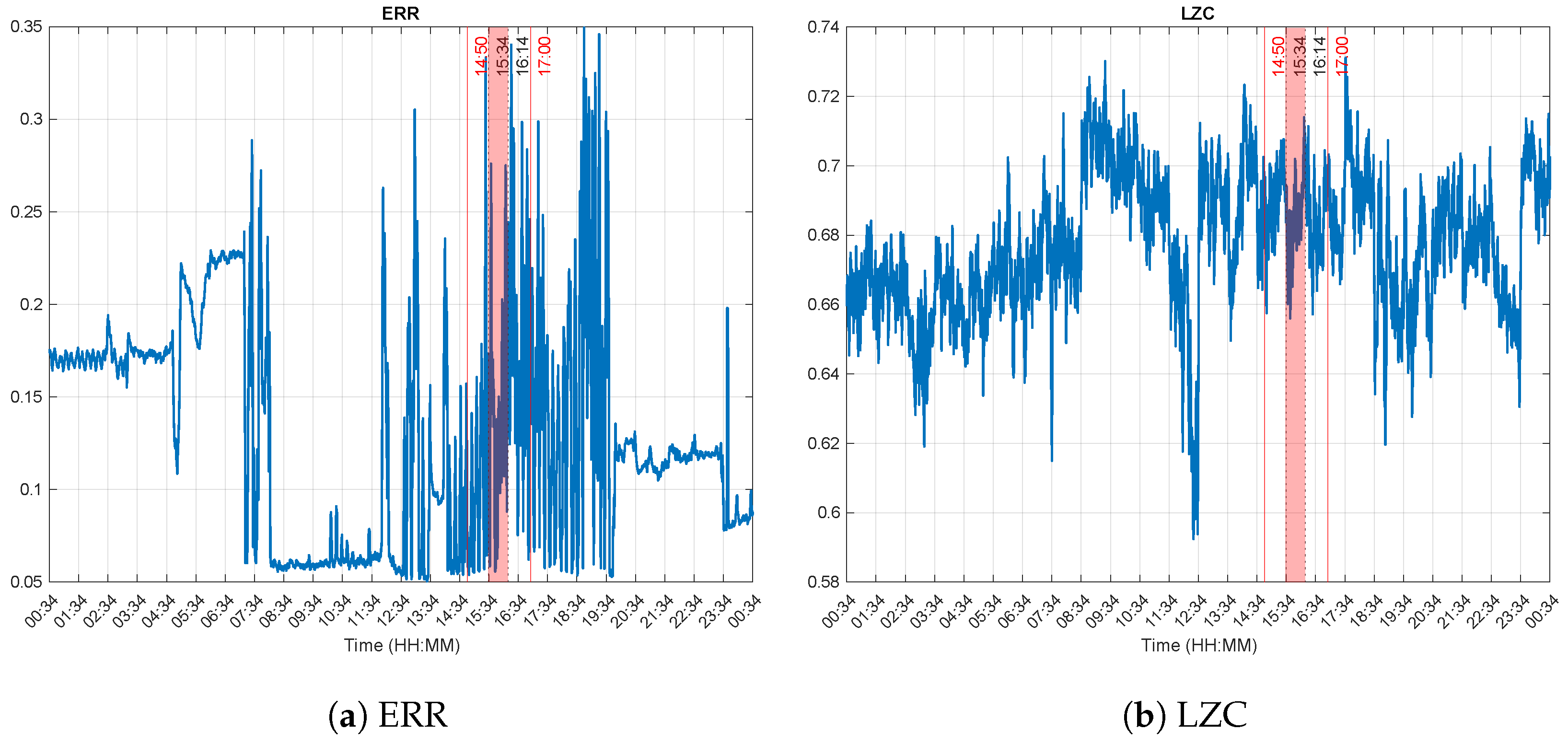
Complexity Features
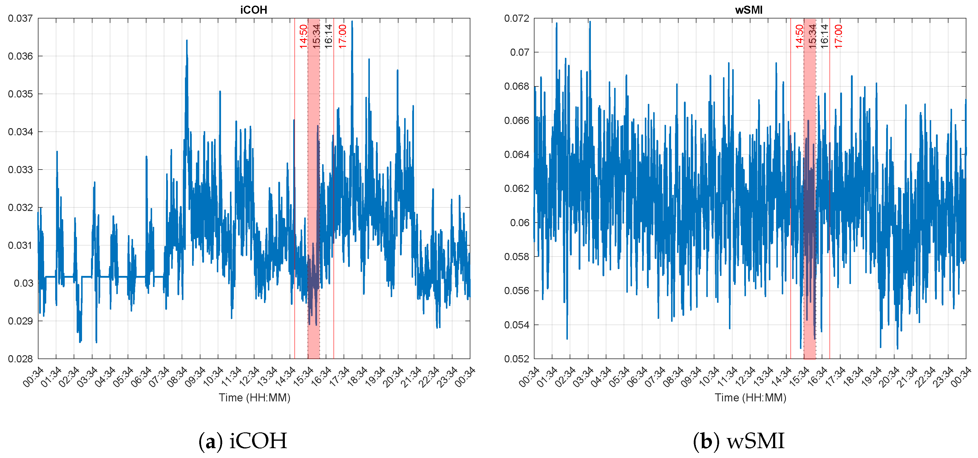
Connectivity Features
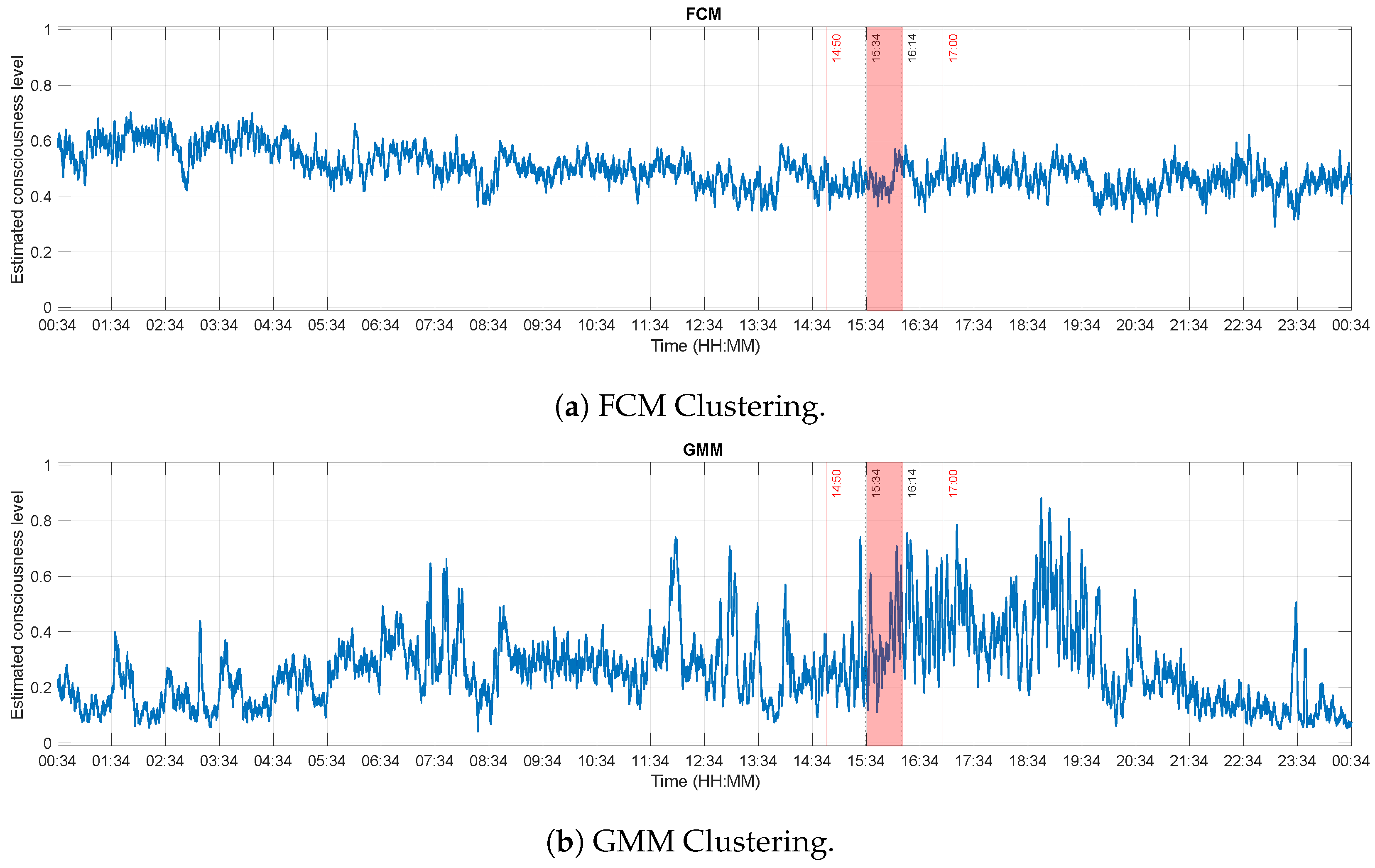
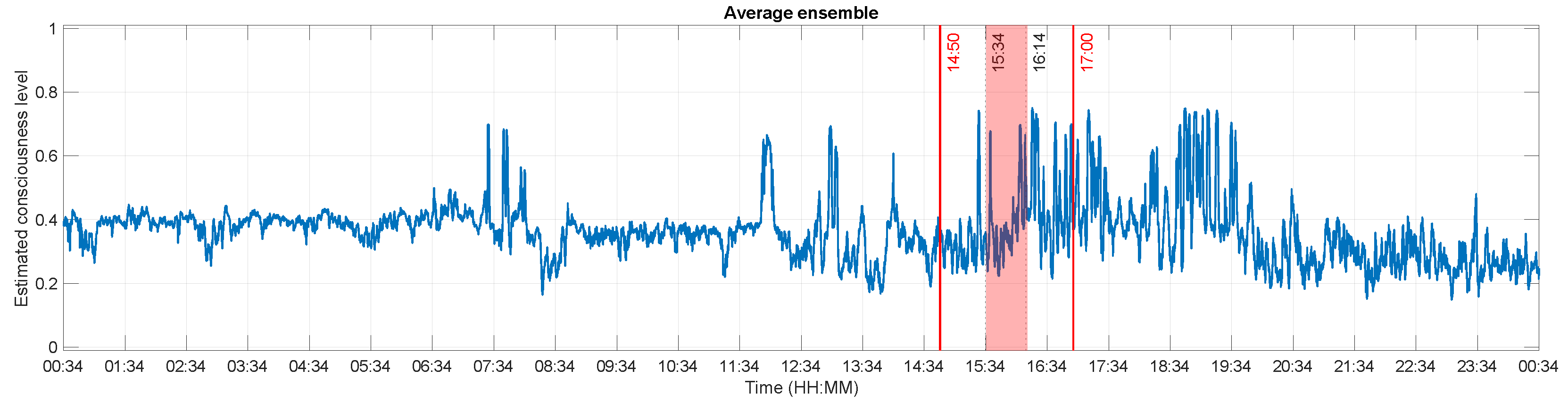
2.2.2. Data Clustering and Consciousness Level Assessment
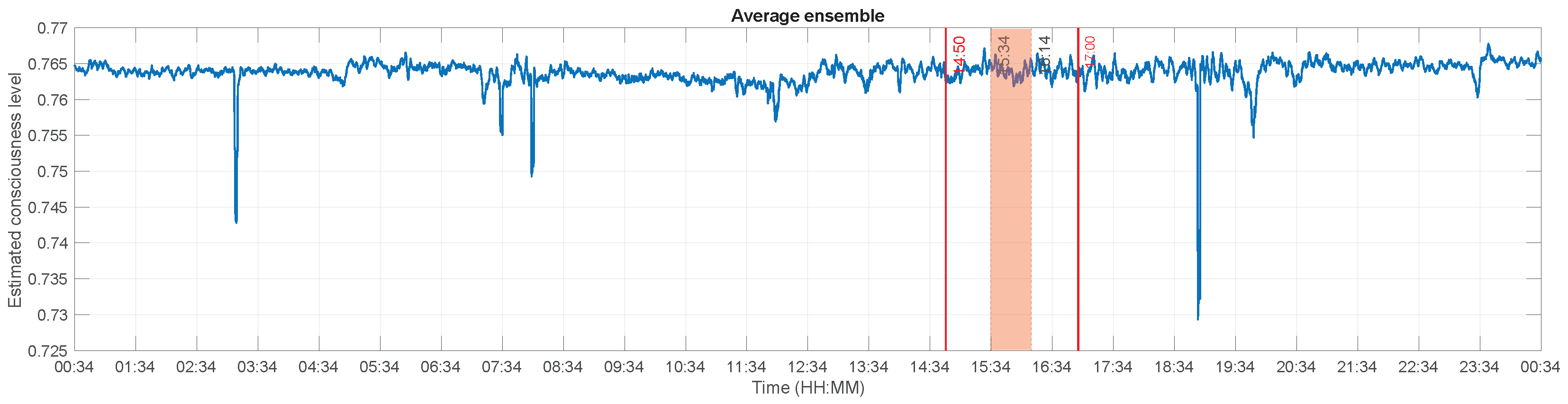
3. Results
4. Discussion
5. Conclusions
Supplementary Materials
Author Contributions
Funding
Data Availability Statement
Acknowledgments
Conflicts of Interest
Abbreviations
| ALS | Amyotrophic Lateral Sclerosis |
| BCI | Brain-Computer Interface |
| CLIS | Completely Locked-In Syndrome |
| DoC | Disorders of Consciousness |
| ECoG | Electrocorticography |
| EEG | Electroencephalography |
| EM | Expectation - Maximisation |
| ERR | Ellipsoid Radius Ratio |
| MCS | Minimally Conscious State |
| PSD | Power Spectral Density |
| SON | Subject’s Own Name |
| SSVEP | Steady-State Visual Evoked Potential |
| SWS | Slow Wave Sleep |
| UWS | Unresponsive Wakefulness Syndrome |
| VS | Vegetative State |
| wSMI | weighted Symbolic Mutual Information |
References
- Bear, M.F.; Connors, B.W.; Paradiso, M.A. Neuroscience: Exploring the Brain, 4th ed.; Wolters Kluwer: Philadelphia, PA, USA, 2016. [Google Scholar]
- Posner, J.B.; Saper, C.B.; Schiff, N.; Plum, F. Plum and Posner’s Diagnosis of Stupor and Coma, 4th ed.; Oxford University Press: Oxford, UK, 2007. [Google Scholar]
- Gosseries, O.; Vanhaudenhuyse, A.; Bruno, M.A.; Demertzi, A.; Schnakers, C.; Boly, M.M.; Maudoux, A.; Moonen, G.; Laureys, S. Disorders of Consciousness: Coma, Vegetative and Minimally Conscious States. In States of Consciousness; Cvetkovic, D., Cosic, I., Eds.; The Frontiers Collection; Springer: Berlin/Heidelberg, Germany, 2011; pp. 29–55. [Google Scholar] [CrossRef] [Green Version]
- Gosseries, O.; Bruno, M.A.; Vanhaudenhuyse, A.; Laureys, S.; Schnakers, C. Consciousness in the Locked-in Syndrome. In The Neurology of Consciousness; Laureys, S., Tononi, G., Eds.; Academic Press: San Diego, CA, USA, 2009; pp. 191–203. [Google Scholar] [CrossRef] [Green Version]
- Kübler, A. The history of BCI: From a vision for the future to real support for personhood in people with locked-in syndrome. Neuroethics 2020, 13, 163–180. [Google Scholar] [CrossRef]
- Kübler, A.; Kotchoubey, B.; Kaiser, J.; Wolpaw, J.R.; Birbaumer, N. Brain-computer communication: Unlocking the locked in. Psychol. Bull. 2001, 127, 358–375. [Google Scholar] [CrossRef]
- Vanhaudenhuyse, A.; Charland-Verville, V.; Thibaut, A.; Chatelle, C.; Tshibanda, J.F.L.; Maudoux, A. Conscious While Being Considered in an Unresponsive Wakefulness Syndrome for 20 Years. Front. Neurol. 2018, 9, 671. [Google Scholar] [CrossRef] [PubMed]
- Lesenfants, D.; Chatelle, C.; Laureys, S.; Noirhomme, Q. Interfaces cerveau-ordinateur, locked-in syndrome et troubles de la conscience. Med. Sci. 2015, 31, 904–911. [Google Scholar] [CrossRef] [Green Version]
- Schnakers, C.; Perrin, F.; Schabus, M.; Hustinx, R.; Majerus, S.; Moonen, G.; Boly, M.; Vanhaudenhuyse, A.; Bruno, M.; Laureys, S. Detecting consciousness in a total locked-in syndrome: An active event-related paradigm. Neurocase 2009, 15, 271–277. [Google Scholar] [CrossRef] [Green Version]
- Bruno, M.A.; Vanhaudenhuyse, A.; Thibaut, A.; Moonen, G.; Laureys, S. From unresponsive wakefulness to minimally conscious PLUS and functional locked-in syndromes: Recent advances in our understanding of disorders of consciousness. J. Neurol. 2011, 258, 1373–1384. [Google Scholar] [CrossRef] [PubMed]
- Combaz, A.; Chatelle, C.; Robben, A.; Vanhoof, G.; Goeleven, A.; Thijs, V.; Van Hulle, M.M.; Laureys, S. A comparison of two spelling Brain-Computer Interfaces based on visual P3 and SSVEP in Locked-In Syndrome. PLoS ONE 2013, 8, e73691. [Google Scholar] [CrossRef] [Green Version]
- Perrin, F.; Schnakers, C.; Schabus, M.; Degueldre, C.; Goldman, S.; Brédart, S.; Faymonville, M.E.; Lamy, M.; Moonen, G.; Luxen, A.; et al. Brain Response to One’s Own Name in Vegetative State, Minimally Conscious State, and Locked-in Syndrome. Arch. Neurol. 2006, 63, 562–569. [Google Scholar] [CrossRef] [PubMed]
- Zhang, Y.; Li, R.; Du, J.; Huo, S.; Hao, J.; Song, W. Coherence in P300 as a predictor for the recovery from disorders of consciousness. Neurosci. Lett. 2017, 653, 332–336. [Google Scholar] [CrossRef]
- Pan, J.; Xie, Q.; He, Y.; Wang, F.; Di, H.; Laureys, S.; Yu, R.; Li, Y. Detecting awareness in patients with disorders of consciousness using a hybrid brain-computer interface. J. Neural Eng. 2014, 11, 056007. [Google Scholar] [CrossRef]
- Guger, C.; Spataro, R.; Allison, B.Z.; Heilinger, A.; Ortner, R.; Cho, W.; La Bella, V. Complete Locked-in and Locked-in Patients: Command Following Assessment and Communication with Vibro-Tactile P300 and Motor Imagery Brain-Computer Interface Tools. Front. Neurol. 2017, 11, 251. [Google Scholar] [CrossRef] [PubMed]
- Murguialday, A.R.; Hill, J.; Bensch, M.; Martens, S.; Halder, S.; Nijboer, F. Transition from the locked in to the completely locked-in state: A physiological analysis. Clin. Neurophysiol. 2011, 122, 925–933. [Google Scholar] [CrossRef] [PubMed]
- Soekadar, S.R.; Born, J.; Birbaumer, N.; Bensch, M.; Halder, S.; Murguialday, A.R. Fragmentation of slow wave sleep after onset of complete locked-in state. J. Clin. Sleep Med. 2013, 9, 951–953. [Google Scholar] [CrossRef] [Green Version]
- Oostenveld, R.; Fries, P.; Maris, E.; Schoffelen, J.M. FieldTrip: Open Source Software for Advanced Analysis of MEG, EEG and Invasive Electrophysiological Data. Comput. Intell. Neurosci. 2001, 2011, 156869. [Google Scholar] [CrossRef]
- Adama, V.S.; Wu, S.J.; Nicolaou, N.; Bogdan, M. Extendable Hybrid approach to detect conscious states in a CLIS patient using machine learning. Simul. Notes Eur. SNE 2022, 32, 37–45. [Google Scholar] [CrossRef]
- Adama, S. Consciousness Level Assessment in Completely Locked-in Syndrome Patients Using Soft Clustering. Ph.D. Thesis, Leipzig University, Leipzig, Germany, 2022. [Google Scholar]
- Gazzaniga, M.S.; Ivry, R.B.; Mangun, G.R. Cognitive Neuroscience: The Biology of the Mind, 5th ed.; W. W. Norton & Company: New York, NY, USA, 2018. [Google Scholar]
- Engemann, D.A.; Raimondo, F.; King, J.R.; Rohaut, B.; Louppe, G.; Faugeras, F.; Annen, J.; Cassol, H.; Gosseries, O.; Fernandez-Slezak, D.; et al. Robust EEG-based cross-site and cross-protocol classification of states of consciousness. Brain 2018, 141, 3179–3192. [Google Scholar] [CrossRef] [PubMed] [Green Version]
- Borjigin, J.; Lee, U.; Liu, T.; Pal, D.; Huff, S.; Klarr, D.; Sloboda, J.; Hernandez, J.; Wang, M.M.; Mashour, G.A. Surge of neurophysiological coherence and connectivity in the dying brain. Proc. Natl. Acad. Sci. USA 2013, 110, 14432–14437. [Google Scholar] [CrossRef] [Green Version]
- Pal, D.; Hambrecht-Wiedbusch, V.S.; Silverstein, B.H.; Mashour, G.A. Electroencephalographic coherence and cortical acetylcholine during ketamine-induced unconsciousness. Br. J. Anaesth. 2015, 114, 979–989. [Google Scholar] [CrossRef]
- Niedermeyer, E. The normal EEG of the waking adult. In Electroencephalography: Basic Principles, Clinical Applications, and Related Fields, 5th ed.; Niedermeyer, E., da Silva, F.L., Eds.; Lippincott Williams & Wilkins (LWW): Philadelphia, PA, USA, 2005; pp. 167–192. [Google Scholar] [CrossRef]
- Stoica, P.; Moses, R.L. Spectral Analysis of Signals; Prentice Hall: Hoboken, NJ, USA, 2005. [Google Scholar]
- Welch, P. The use of fast Fourier transform for the estimation of power spectra: A method based on time averaging over short, modified periodograms. IEEE Trans. Audio Electroacoust. 1967, 15, 70–73. [Google Scholar] [CrossRef] [Green Version]
- Imtiaz, S.A.; Rodriguez-Villegas, E. A Low Computational Cost Algorithm for REM Sleep Detection Using Single Channel EEG. Ann. Biomed. Eng. 2014, 42, 2344–2359. [Google Scholar] [CrossRef] [Green Version]
- Abootalebi, V.; Moradi, M.H.; Khalilzadeh, M.A. A new approach for EEG feature extraction in P300-based lie detection. Comput. Methods Programs Biomed. 2009, 94, 48–57. [Google Scholar] [CrossRef] [PubMed]
- Rampil, I.J.; Sasse, F.J.; Smith, N.T.; Hoff, B.H.; Flemming, D.C. Spectral edge frequency—A new correlate of anesthetic depth. Anesthesiology 1980, 53, S12. [Google Scholar] [CrossRef]
- Touchard, C.; Cartailler, J.; Levé, C.; Parutto, P.; Buxin, C.; Garnot, L.; Matéo, J.; Kubis, N.; Mebazaa, A.; Gayat, E.; et al. EEG power spectral density under Propofol and its association with burst suppression, a marker of cerebral fragility. Clin. Neurophysiol. 2019, 130, 1311–1319. [Google Scholar] [CrossRef]
- Najarian, K.; Splinter, R. Biomedical Signal and Image Processing, 1st ed.; CRC Press: Boca Raton, FL, USA, 2005. [Google Scholar]
- Hayashi, K.; Mukai, N.; Sawa, T. Poincaré analysis of the electroencephalogram during sevoflurane anesthesia. Clin. Neurophysiol. 2014, 126, 404–411. [Google Scholar] [CrossRef]
- Eagleman, S.L.; Vaughn, D.A.; Drover, D.R.; Drover, C.M.; Cohen, M.S.; Ouellette, N.T.; MacIver, M.B. Do Complexity Measures of Frontal EEG Distinguish Loss of Consciousness in Geriatric Patients Under Anesthesia? Front. Neurosci. 2018, 12, 645. [Google Scholar] [CrossRef]
- Satti, R.; Abid, N.U.H.; Bottaro, M.; Rui, M.D.; Garrido, M.; Raoufy, M.R.; Montagnese, S.; Mani, A.R. The Application of the Extended Poincaré Plot in the Analysis of Physiological Variabilities. Front. Physiol. 2019, 10, 116. [Google Scholar] [CrossRef]
- Lempel, A.; Ziv, J. On the Complexity of Finite Sequences. IEEE Trans. Inf. Theory 1976, 22, 75–81. [Google Scholar] [CrossRef]
- Schartner, M.; Seth, A.; Noirhomme, Q.; Boly, M.; Bruno, M.A.; Laureys, S.; Barrett, A. Complexity of Multi-Dimensional Spontaneous EEG Decreases during Propofol Induced General Anaesthesia. PLoS ONE 2015, 10, e0133532. [Google Scholar] [CrossRef]
- Aboy, M.; Hornero, R.; Abasolo, D.; Alvarez, D. Interpretation of the Lempel-Ziv Complexity Measure in the Context of Biomedical Signal Analysis. IEEE Trans. Biomed. Eng. 2006, 53, 2282–2288. [Google Scholar] [CrossRef] [PubMed] [Green Version]
- Pullon, R.M.; Yan, L.; Sleigh, J.W.; Warnaby, C.E. Granger Causality of the Electroencephalogram Reveals Abrupt Global Loss of Cortical Information Flow during Propofol-induced Loss of Responsiveness. Anesthesiology 2020, 133, 774–786. [Google Scholar] [CrossRef]
- Bourdillon, P.; Hermann, B.; Guénot, M.; Bastuji, H.; Isnard, J.; King, J.R.; Sitt, J.; Naccache, L. Brain-scale cortico-cortical functional connectivity in the delta-theta band is a robust signature of conscious states: An intracranial and scalp EEG study. Sci. Rep. 2020, 10, 14037. [Google Scholar] [CrossRef]
- Kayser, A.S.; Sun, F.T.; D’Esposito, M. A comparison of Granger causality and coherency in fMRI-based analysis of the motor system. Hum. Brain Mapp. 2009, 30, 3475–3494. [Google Scholar] [CrossRef] [PubMed] [Green Version]
- Sakellariou, D.; Koupparis, A.M.; Kokkinos, V.; Koutroumanidis, M.; Kostopoulos, G.K. Connectivity Measures in EEG Microstructural Sleep Elements. Front. Neuroinform. 2016, 10, 5. [Google Scholar] [CrossRef] [Green Version]
- Nolte, G.; Bai, O.; Wheaton, L.; Mari, Z.; Vorbach, S.; Hallett, M. Identifying true brain interaction from EEG data using the imaginary part of coherency. Clin. Neurophysiol. 2004, 115, 2292–2307. [Google Scholar] [CrossRef] [PubMed]
- Blinowska, K.J.; Zygierewicz, J. Practical Biomedical Signal Analysis Using MATLAB, 1st ed.; CRC Press, Inc.: Boca Raton, FL, USA, 2011. [Google Scholar]
- Priestley, M.B. Spectral Analysis and Time Series, Two-Volume Set: Volumes I and II; Both volumes bound together; Elsevier Science: Amsterdam, The Netherlands, 1981. [Google Scholar]
- Sanei, S.; Chambers, J.A. EEG Signal Processing; Wiley: Chichester, West Sussex, UK, 2013. [Google Scholar]
- da Silva, F.L. EEG Analysis: Theory and Practice. In Electroencephalography: Basic Principles, Clinical Applications, and Related Fields, 5th ed.; Niedermeyer, E., da Silva, F.L., Eds.; Lippincott Williams & Wilkins (LWW): Philadelphia, PA, USA, 2005; pp. 1199–1232. [Google Scholar]
- Lee, U.; Blain-Moraes, S.; Mashour, G.A. Assessing levels of consciousness with symbolic analysis. Phil. Trans. R. Soc. A 2015, 373, 20140117. [Google Scholar] [CrossRef] [PubMed]
- King, J.R.; Sitt, J.D.; Faugeras, S. Information Sharing in the Brain Indexes Consciousness in Non-communicative Patients. Curr. Biol. 2013, 23, 1914–1919. [Google Scholar] [CrossRef] [PubMed] [Green Version]
- Assiri, A.S.; Nazir, S.; Velastin, S.A. Breast Tumor Classification Using an Ensemble Machine Learning Method. J. Imaging 2020, 6, 39. [Google Scholar] [CrossRef]
- Sherazi, S.W.A.; Bae, J.W.; Lee, J.Y. A soft voting ensemble classifier for early prediction and diagnosis of occurrences of major adverse cardiovascular events for STEMI and NSTEMI during 2-year follow-up in patients with acute coronary syndrome. PLoS ONE 2021, 16, e0249338. [Google Scholar] [CrossRef]
- Peters, G.; Crespo, F.; Lingras, P.; Weber, R. Soft clustering—Fuzzy and rough approaches and their extensions and derivatives. Int. J. Approx. Reason. 2013, 54, 307–322. [Google Scholar] [CrossRef]
- Bezdek, J.C. Pattern Recognition with Fuzzy Objective Function Algorithms, 1st ed.; Springer: Boston, MA, USA, 1981. [Google Scholar] [CrossRef]
- Chiu, S.L. Fuzzy Model Identification Based on Cluster Estimation. J. Intell. Fuzzy Syst. 1994, 2, 267–278. [Google Scholar] [CrossRef]
- Ferraro, M.B.; Giordani, P. Soft clustering. WIREs Comput. Stat. 2020, 12, e1480. [Google Scholar] [CrossRef]
- Stahl, D.; Sallis, H. Model-based cluster analysis. WIREs Comput. Stat. 2012, 4, 341–358. [Google Scholar] [CrossRef]
- Wu, S.J.; Nicolaou, N.; Bogdan, M. Consciousness Detection in a Complete Locked-in Syndrome Patient through Multiscale Approach Analysis. Entropy 2020, 22, 1411. [Google Scholar] [CrossRef] [PubMed]
- Schober, P.; Boer, C.; Schwarte, L.A. Correlation Coefficients: Appropriate Use and Interpretation. Anesth Analg. 2018, 126, 1763–1768. [Google Scholar] [CrossRef]


| Time | Interval | Consciousness Level (Self) | Consciousness Level (Pre-Defined) |
|---|---|---|---|
| All (24 h) | 00:34 to 00:34 | 0.3829 | 0.7638 |
| Before experiment | 00:34 to 14:50 | 0.3879 | 0.7635 |
| During experiment | 14:50 to 17:00 | 0.4078 | 0.7640 |
| “conscious” time | 15:34 to 16:14 | 0.4084 | 0.7639 |
| After experiment | 17:00 to 00:34 | 0.3663 | 0.7651 |
| FCM | GMM | Ensemble | |
|---|---|---|---|
| −0.2872 | −0.403 | −0.4919 | |
| 0.8906 | −0.2793 | 0.3579 | |
| SEF95 | 0.3949 | −0.546 | 0.1881 |
| ERR | 0.2812 | 0.165 | 0.3316 |
| LZC | 0.4416 | 0.17 | 0.2849 |
| 0.0203 | 0.0098 | 0.0188 | |
| wSMI | 0.1428 | 0.346 | 0.3238 |
Disclaimer/Publisher’s Note: The statements, opinions and data contained in all publications are solely those of the individual author(s) and contributor(s) and not of MDPI and/or the editor(s). MDPI and/or the editor(s) disclaim responsibility for any injury to people or property resulting from any ideas, methods, instructions or products referred to in the content. |
© 2022 by the authors. Licensee MDPI, Basel, Switzerland. This article is an open access article distributed under the terms and conditions of the Creative Commons Attribution (CC BY) license (https://creativecommons.org/licenses/by/4.0/).
Share and Cite
Adama, S.; Bogdan, M. Application of Soft-Clustering to Assess Consciousness in a CLIS Patient. Brain Sci. 2023, 13, 65. https://doi.org/10.3390/brainsci13010065
Adama S, Bogdan M. Application of Soft-Clustering to Assess Consciousness in a CLIS Patient. Brain Sciences. 2023; 13(1):65. https://doi.org/10.3390/brainsci13010065
Chicago/Turabian StyleAdama, Sophie, and Martin Bogdan. 2023. "Application of Soft-Clustering to Assess Consciousness in a CLIS Patient" Brain Sciences 13, no. 1: 65. https://doi.org/10.3390/brainsci13010065