
Indexes for the E-Baking Tray Task: A Look on Laterality, Verticality and Quality of Exploration

 , ,
, ,
Abstract
:1. Introduction
- new indexes (e.g., between distance from optimal sequences) [11]. These indexes were developed specifically for E-BTT data and can be generalized to all tasks that involves coordinates.
2. Materials and Methods
2.1. Participants
2.2. Measures
2.2.1. Enhanced Baking Tray Task
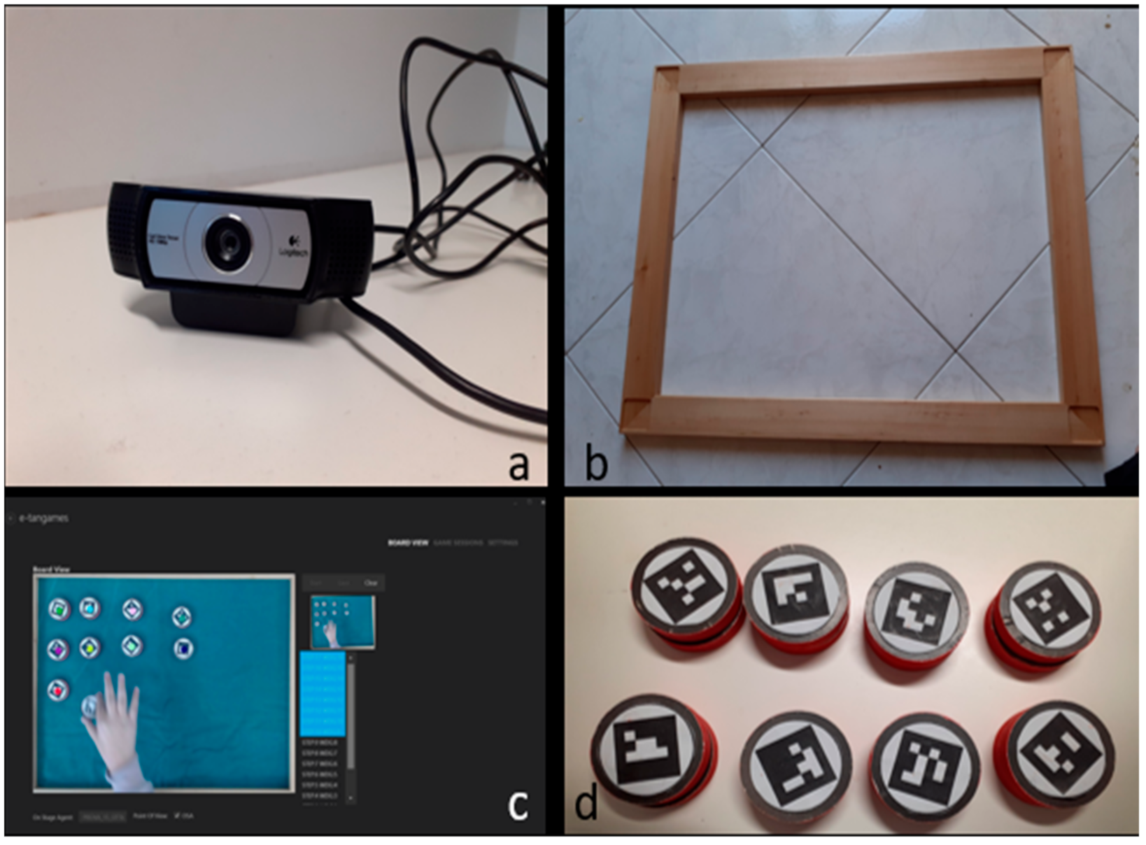
- Cubes were replaced by disks because the camera worked better with flat objects; moreover, cubes were subject to an aggregation bias (that is, putting all cubes close to form another object). Disks measured 5 cm in diameter.
- ArUco marker tags on each disk and frame’s corner [7]. They consisted of a black-and-white matrix, similar to QrCodes.
- A Logitech C930e webcam camera placed above the table, fixed thanks to a metallic arm in order to facilitate object detection.
- E-TAN, the software part of the E-BTT. It is a versatile platform developed ad hoc for the E-BTT but can potentially be applied to many other tasks. It allows tangible interfaces detection inside the “tray” and calculates many important variables, such as the coordinates of each detected disk, along with its time stamp. Moreover, information about each session (board dimension, date, gender and age of the participants) are recorded.
2.2.2. Indexes
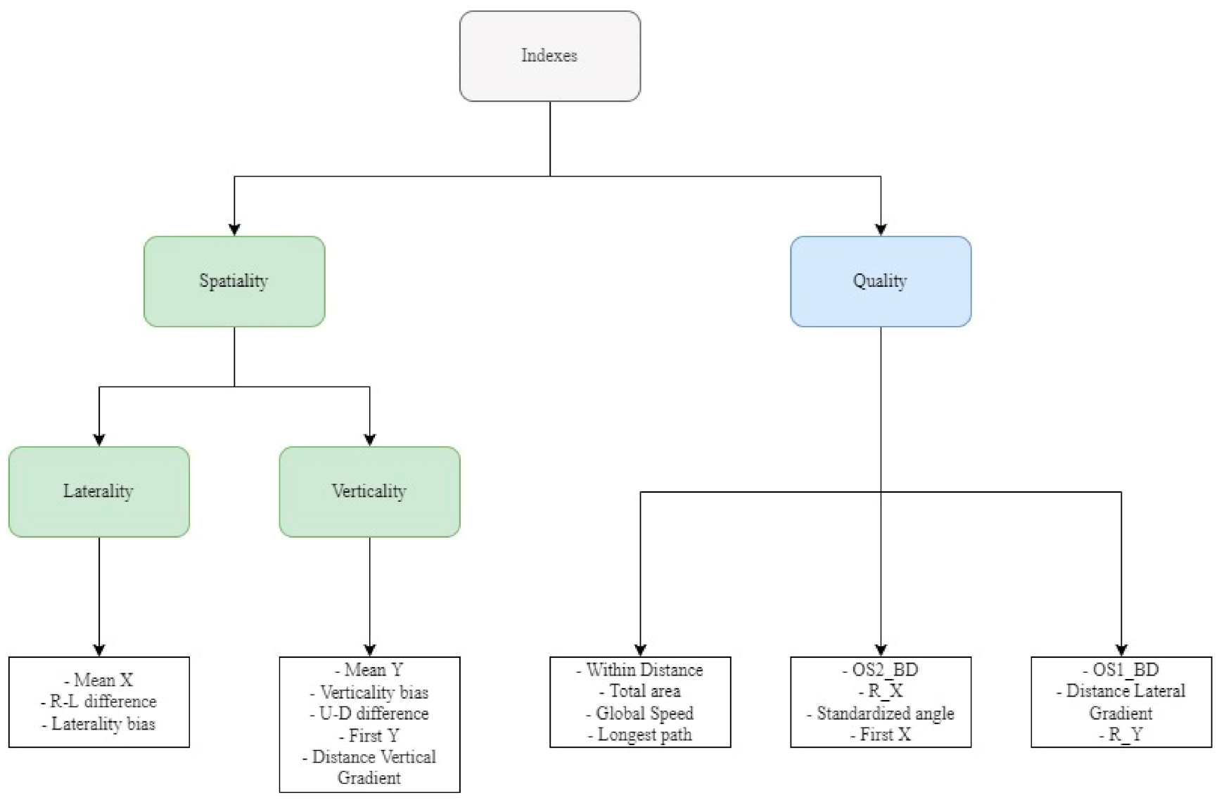
- Spatial indexes. Spatial indexes summarize where the disks were placed. They are further divided in laterality and verticality indexes, depending on which kind of coordinate they were calculated on (X or Y). The quadrant analysis is classified separately since it comprehends both the vertical and the lateral dimensions.
- ◦
- Quadrant analysis (first and last disk). The internal space of the frame is virtually divided in four equal parts based on each axis. The disks’ placement frequencies are counted and analysed through a one-way Pearson’s chi-square in order to reveal where it is more likely to place the first or the last disk. It is also possible to compute a two-way chi-square, considering laterality and verticality as two different variables, but for theoretical reasons, it was preferred not to.Quadrant analysis could be helpful and fast to detect tendency in spatial exploration.
- ◦
- Laterality indexes. All indexes measured using the X coordinates were considered measures of laterality. Laterality indexes gave the idea of how much to the right or to the left one disk or the entire sequence was located. Laterality indexes are as follows:
- ■
- First X. It corresponds to the first placed disk’s X coordinate, in cm. It can be considered an index of pseudoneglect [2]. The rationale behind this was that spatial exploration started asymmetrically, and in fact the first disk was placed leftward.
- ■
- Right/left disks’ difference (R/L difference). The number of disks placed on the left is subtracted from the number of disks placed on the right to obtain an estimate of the imbalance in disks’ placement. A positive number means an asymmetry towards the right while a negative number would mean more disks placed on the left. Zero means symmetry.
- ■
- Laterality bias. The laterality bias (LB) was developed by Facchin and colleagues [10] as the ratio between the right/left cubes difference and their total number, in a percentage. This formula was thoroughly used for coordinate data, considering every left disk had a X coordinate less than −10 and every right disk had a X coordinate more than +10. Facchin and colleagues [10] calculated two cutoff scores using nonparametric tolerance intervals: −12.6% for the left side and +18.8% for the right side.
- ■
- Distance lateral gradient. It was developed by Rabuffetti and colleagues [14]. The gradient was developed to assess possible relationships between test performance and laterality. The slope of the regression line on the intercancellation distance (similar to the “within distance”, see below), putting the lateral coordinate as a predictor, was computed. The slope of the fitting line corresponds to the distance lateral gradient. Please note that only the coordinates from the second one were considered to match the fifteen distances. This index can be interpreted as the variation on the distance between each disk and the next one, moving by one unit (in this case, centimeters) in laterality. A positive gradient means that the more the coordinates vary rightward, the higher the distances will be between each disk and the next one.
- ■
- Center of mass (mean_X). It is calculated as the mean of all 16 coordinates. It gives an idea of how much the overall configuration is biased toward the left or the right. A positive center of mass indicates that the configuration is biased rightward.
- ◦
- Verticality indexes. Verticality was not taken into account in previous studies [4] because vertical neglect is a relatively rare occurrence [16]. Nonetheless, it should be interesting to assess verticality in healthy participants because the role of verticality in visual search is underexplored. Verticality indexes are analogous to their laterality counterparts: first Y, up/down disks’ difference (U/D difference), verticality bias, distance vertical gradient, center of mass (mean_Y).
- Quality indexes. Quality indexes refer to the final sequence’s quality and organization. Some of them derive from the visual search literature on cancellation tasks [12,13,14,15]. Visual search organization was initially investigated mainly with patients with unilateral brain injury (especially in the right hemisphere, with or without unilateral neglect), highlighting how they tended to describe irregular exploratory patterns whereas neurologically healthy subjects had a more organized and regular pattern of cancellation [12,15,17,18,19,20]. Mark and colleagues [12], in fact, tried to quantify the spatial organization in a Star Cancellation task in patients who had suffered a stroke with three indexes. Subsequently, other authors [13,14] used the same indexes and formulated new ones, always applying them to the task of cancellation of stimuli. For the E-BTT task, we chose to use the following indexes: number of intersection (intersection rate, longest path), global speed, best R and standardized angle.
- ■
- Total area. The proportion of explored area was calculated through the Monte Carlo integration algorithm. In particular, the convex hull polygon delimited by the disks’ sequence (for more detail, please refer to [3]) was considered. Since outliers in disks’ placement could alter the estimate, the external and internal polygon were averaged. In Cerrato and colleagues, the log transformation of the portion of explored area was divided into a left and a right portion. This index proved to be useful to discriminate patients from healthy subjects: only 8% of healthy participants had a pathological area. The quantity of occupied space inside the frame could be an index of performance quality.
- ■
- Total time. In this study, performance time was calculated as the time interval between the placement of the final and the first disk. It could be regarded as a (dis)organization index since difficulties of spatial exploration should lead to longer execution times. In cancellation tasks, performance time was used as a sustained attention measure [13].
- ■
- Within distance (WD). Within distance was the sum of the Euclidean distances between each disk and the next one. It can be regarded as the measure of total distance of explored space with the disks. It was recently used as an organization measure in Argiuolo and colleagues [11], but a similar index was previously applied to the cancellation task by several other authors [12,13,14]. In these cases, it was calculated as the distance (with the Euclidean formula) between each cancelled mark and the next one, excluding perseverations. This serves as an organized path meant to minimize the distance between the newly cancelled item and the one which the participant will decide to mark next.
- ■
- Number of intersections, intersections rate, longest path. These three indexes refer to the same construct, so they are placed together. The number of intersections is the sum of each intersection into the imaginary line that links each disk to the next one. The intersection rate is calculated averaging the number of intersections (that is, dividing it for the 15 segments) while the longest path is the highest number, for each sequence, of intersections-free lines. In other words, if a pattern contains no intersection, the longest path is 15. These indexes were used by several authors as a visual search organization measure [12,13,14]. Conceptually, a good quality sequence should not come back to the same spatial position as before; that is, the sequence should not intersect with itself.
- ■
- Global speed. Global speed is calculated as the ratio between the within distance and the total time. Virtually, the lower the speed, the more disorganized the pattern should be.
- ■
- Best R (R_X and R_Y). The vast majority of healthy participants cancelled items with a horizontal or vertical movement (that is, by rows or by columns) [17,18,20]. This was also common for the E-BTT (see [11] for more details). To address this, Mark and colleagues created the best R, the highest, in absolute value, among the two Pearson correlations between the coordinates (X and Y separately) and their order. The main limitation of this approach was that this index did not catch patterns other than orthogonal ones, for example, spiral paths. A further limitation is that choosing to use only the highest between two values makes it impossible to know which one is horizontal or vertical. We chose to use both correlation coefficients.
- ■
- Standardized angle. As an integration to the information given by the best R, Dalmaijer [13] developed a standardized measure of the mean angle of the patterns’ segments. The angle between two points is calculated as the arcsin of the ratio between the vertical distance (the difference between the two Ys) between two points and their Euclidean distance. Then, each angle is standardized and averaged. The higher the standardized angle, the more efficient the pattern should be.
- ■
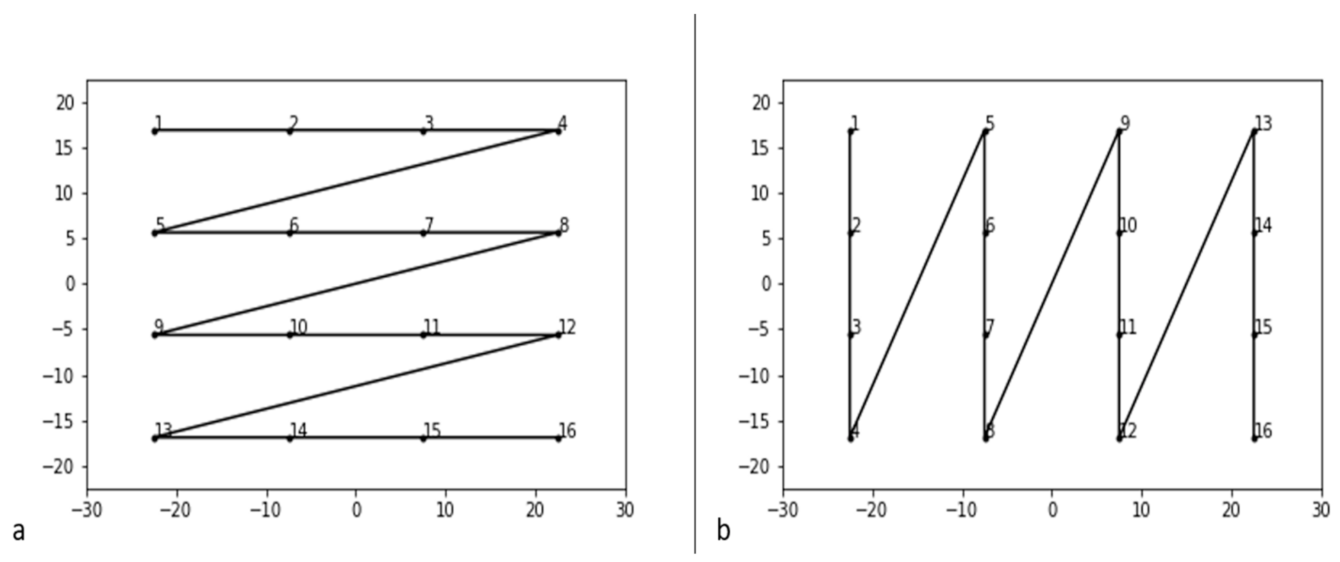
- Between distance from optimal sequences. This last index was proposed recently based on the results shown in Argiuolo and colleagues [11]. It consisted of the “between distance”—or the distance between the corresponding disks of two distinct sequences—from sequences that could be considered optimal. They were created based on the fact that as for the E-BTT, the goal of the task was to place the disks inside the frame as evenly as possible. Therefore, the optimal disposition should occupy as much space as possible. The 16 disks’ coordinates were calculated by dividing the available area in 16 equal parts. The result was an optimal disposition of four per four disks; the only variable now was the sequence of disposition. Following the examples from cancellation tasks, we wondered whether the sequence by rows and columns was also applicable for the E-BTT. Indeed, the most frequent sequences in Argiuolo and colleagues’ [11] groups were the first two groups where a sawtooth was the final result. The sawtooth goes by rows and columns, similar to a commonly used cancellation path reported by Warren, Moore and Vogtle [18]. Therefore, we chose these two sequences as optima and calculated the BDs from them (Figure 2). The results were two indexes that gave an idea of how different each particular sequence was from the optimal ones. Of course, this choice had limitations; future research could take this into account and also consider other optimal sequences.
2.3. Data Analysis
3. Results
3.1. Right/Left Asymmetry
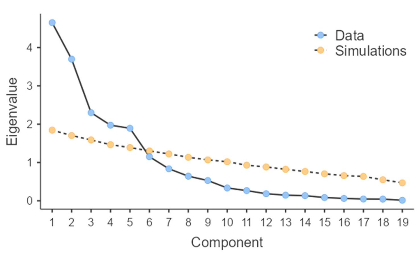
3.2. Indexes’ Structure
- A component classifiable as verticality (mean Y, verticality bias, U/D difference, first Y, distance vertical gradient) and a component of laterality (mean X, laterality bias, R/L difference).
- An “explored space/quality” component made up of within distance, total area, global speed and longest path.
- A component consisting of the distance from the first optimal sequence (OS1_BD), the distance lateral gradient (DLG) and the correlation between Y coordinates and their order (R_Y).
- Similarly, the distance from the second optimal sequence (OS2_BD), the correlation between X coordinates and their order (R_X), the angle (standardized angle) and the first X goes into the second component.
4. Discussion and Conclusions
Author Contributions
Funding
Institutional Review Board Statement
Informed Consent Statement
Data Availability Statement
Acknowledgments
Conflicts of Interest
Appendix A

References
- Tham, K.; Tegnér, R. The baking tray task: A test of spatial neglect. Neuropsychol. Rehabil. 1996, 6, 19–26. [Google Scholar] [CrossRef] [PubMed]
- Somma, F.; Argiuolo, A.; Cerrato, A.; Ponticorvo, M.; Mandolesi, L.; Miglino, O.; Bartolomeo, P.; Gigliotta, O. Valutazione dello pseudoneglect mediante strumenti tangibili e digitali [Pseudoneglect evaluation using tangible and digital tools]. Sist. Intell. 2020, 32, 533–549. [Google Scholar] [CrossRef]
- Cerrato, A.; Pacella, D.; Palumbo, F.; Beauvais, D.; Ponticorvo, M.; Miglino, O.; Bartolomeo, P. E-TAN, a technology-enhanced platform with tangible objects for the assessment of visual neglect: A multiple single-case study. Neuropsychol. Rehabil. 2020, 31, 1130–1144. [Google Scholar] [CrossRef] [PubMed]
- Cerrato, A.; Ponticorvo, M.; Gigliotta, O.; Bartolomeo, P.; Miglino, O. Btt-scan: Uno strumento per la valutazione della negligenza spaziale unilaterale [Btt-scan: A tool for the assessment of unilateral spatial negligence]. Sist. Intell. 2019, 31, 253–270. [Google Scholar] [CrossRef]
- Cerrato, A.; Ponticorvo, M.; Gigliotta, O.; Bartolomeo, P.; Miglino, O. The Assessment of Visuospatial Abilities with Tangible Interfaces and Machine Learning. In Understanding the Brain Function and Emotions; Ferrández Vicente, J., Álvarez-Sánchez, J., de la Paz López, F., Toledo Moreo, J., Adeli, H., Eds.; IWINAC 2019, Lecture Notes in Computer Science; Springer: Cham, Switzerland, 2019; Volume 11486. [Google Scholar] [CrossRef]
- Gentile, C.; Cerrato, A.; Ponticorvo, M. Using technology and tangible interfaces in a visuospatial cognition task: The case of the Baking Tray Task. CEUR Workshop Proc. 2019, 2524, 1–9. [Google Scholar]
- Garrido-Jurado, S.; Muñoz-Salinas, R.; Madrid-Cuevas, F.J.; Marín-Jiménez, M.J. Automatic generation and detection of highly reliable fiducial markers under occlusion. Pattern Recogn. 2014, 47, 2280–2292. [Google Scholar] [CrossRef]
- Karnath, H.O.; Himmelbach, M.; Rorden, C. The subcortical anatomy of human spatial neglect: Putamen, caudate nucleus and pulvinar. Brain 2002, 125, 350–360. [Google Scholar] [CrossRef] [PubMed] [Green Version]
- Natale, E.; Marzi, C.A.; Bricolo, E.; Johannsen, L.; Karnath, H.-O. Abnormally speeded saccades to ipsilesional targets in patients with spatial neglect. Neuropsychologia 2007, 45, 263–272. [Google Scholar] [CrossRef]
- Facchin, A.; Beschin, N.; Pisano, A.; Reverberi, C. Normative data for distal line bisection and baking tray task. Neurol. Sci. 2016, 37, 1531–1536. [Google Scholar] [CrossRef]
- Argiuolo, A.; Somma, F.; Marocco, D.; Gigliotta, O.; Bartolomeo, P.; Miglino, O.; Ponticorvo, M. Abstracts and authors of the 8th International Conference on Spatial Cognition: Cognition and Action in a Plurality of Spaces (ICSC 2021). Cogn. Process 2021, 22, 3–67. [Google Scholar] [CrossRef]
- Mark, V.W.; Woods, A.J.; Ball, K.K.; Roth, D.L.; Mennemeier, M. Disorganized search on cancellation is not a consequence of neglect. Neurology 2004, 63, 78–84. [Google Scholar] [CrossRef] [Green Version]
- Dalmaijer, E.S.; Van der Stigchel, S.; Nijboer, T.C.W.; Cornelissen, T.H.W.; Husain, M. CancellationTools: All-in-one software for administration and analysis of cancellation tasks. Behav. Res. Methods 2015, 47, 1065–1075. [Google Scholar] [CrossRef] [Green Version]
- Rabuffetti, M.; Farina, E.; Alberoni, M.; Pellegatta, D.; Appollonio, I.; Affanni, P.; Forni, M.; Ferrarin, M. Spatio-temporal features of visual exploration in unilaterally brain-damaged subjects with or without neglect: Results from a touchscreen test. PLoS ONE 2012, 7, e031511. [Google Scholar] [CrossRef]
- Woods, A.J.; Mark, V.W. Convergent validity of executive organization measures on cancellation. J. Clin. Exp. Neuropsychol. 2007, 29, 719–723. [Google Scholar] [CrossRef]
- Morris, M.; Mańkowska, A.; Heilman, K.M. Upper Vertical Spatial Neglect With A Right Temporal Lobe Stroke. Cogn. Behav. Neurol. 2020, 33, 63–66. [Google Scholar] [CrossRef]
- Donnelly, N.; Guest, R.; Fairhurst, M.; Potter, J.; Deighton, A.; Patel, M. Developing algorithms to enhance the sensitivity of cancellation tests of visuospatial neglect. Behav. Res. Methods Instrum. Comput. 1999, 31, 668–673. [Google Scholar] [CrossRef] [Green Version]
- Gauthier, L.; Dehaut, F.; Joanette, Y. The Bells Test: A quantitative and qualitative test for visual neglect. Int. J. Clin. Neuropsyc. 1989, 11, 49–54. [Google Scholar]
- Warren, M.; Moore, J.M.; Vogtle, L.K. Search performance of healthy adults on cancellation tests. Am. J. Occup. Ther. 2008, 62, 588–594. [Google Scholar] [CrossRef] [Green Version]
- Weintraub, S.; Mesulam, M.M. Visual hemispatial inattention: Stimulus parameters and exploratory strategies. J. Neurol. Neurosurg. Psychiatry 1988, 51, 1481–1488. [Google Scholar] [CrossRef] [Green Version]
- Jamovi. (Version 2.2). Available online: https://www.jamovi.org (accessed on 30 August 2021).
- Kaiser, H.F. An index of factorial simplicity. Psychometrika 1974, 39, 31–36. [Google Scholar] [CrossRef]
- Field, A.P. Discovering Statistics Using SPSS (and Sex and Drugs and Rock’ n’ Roll), 3rd ed.; Sage: London, UK, 2009. [Google Scholar]
- Horn, J.L. A rationale and test for the number of factors in factor analysis. Psychometrika 1965, 30, 179–185. [Google Scholar] [CrossRef]
- Zwick, W.R.; Velicer, W.F. Comparison of five rules for determining the number of components to retain. Psychol. Bull. 1986, 99, 432–442. [Google Scholar] [CrossRef]
- Somma, F.; Bartolomeo, P.; Vallone, F.; Argiuolo, A.; Cerrato, A.; Miglino, O.; Mandolesi, L.; Zurlo, M.C.; Gigliotta, O. Further to the Left: Stress-Induced Increase of Spatial Pseudoneglect During the COVID-19 Lockdown. Front. Psychol. 2021, 12, 573846. [Google Scholar] [CrossRef]
- Bowers, D.; Heilman, K.M. Pseudoneglect: Effects of hemispace on a tactile line bisection task. Neuropsychologia 1980, 18, 491–498. [Google Scholar] [CrossRef]
- Jewell, G.; McCourt, M.E. Pseudoneglect: A review and meta-analysis of performance factors in line bisection tasks. Neuropsychologia 2000, 38, 93–110. [Google Scholar] [CrossRef]
- Gigliotta, O.; Malkinson, T.S.; Miglino, O.; Bartolomeo, P. Pseudoneglect in visual search: Behavioral evidence and connectional constraints in simulated neural circuitry. eNeuro 2017, 4, ENEURO.0154-17.2017. [Google Scholar] [CrossRef] [PubMed] [Green Version]
- Sampaio, E.; Chokron, S. Pseudoneglect and reversed pseudoneglect among left-handers and right-handers. Neuropsychologia 1992, 30, 797–805. [Google Scholar] [CrossRef]
- Bartolomeo, P. Visual neglect. Curr. Opin. Neurol. 2007, 20, 381–386. [Google Scholar] [CrossRef]
- Pérennou, D.A.; Mazibrada, G.; Chauvineau, V.; Greenwood, R.; Rothwell, J.; Gresty, M.A.; Bronstein, A.M. Lateropulsion, pushing and verticality perception in hemisphere stroke: A causal relationship? Brain 2008, 131, 2401–2413. [Google Scholar] [CrossRef] [Green Version]
- Utz, K.S.; Keller, I.; Artinger, F.; Stumpf, O.; Funk, J.; Kerkhoff, G. Multimodal and multispatial deficits of verticality perception in hemispatial neglect. Neuroscience 2011, 188, 68–79. [Google Scholar] [CrossRef]
- Pérennou, D.; Piscicelli, C.; Barbieri, G.; Jaeger, M.; Marquer, A.; Barra, J. Measuring verticality perception after stroke: Why and how? Neurophysiol. Clin./Clin. Neurophysiol. 2014, 44, 25–32. [Google Scholar] [CrossRef]
- Fukata, K.; Amimoto, K.; Fujino, Y.; Inoue, M.; Inoue, M.; Takahashi, Y.; Sekine, D.; Makita, S.; Takahashi, H. Influence of unilateral spatial neglect on vertical perception in post-stroke pusher behavior. Neurosci. Lett. 2020, 715, 134667. [Google Scholar] [CrossRef]
- Saj, A.; Honoré, J.; Davroux, J.; Coello, Y.; Rousseaux, M. Effect of Posture on the Perception of Verticality in Neglect Patients. Stroke 2005, 36, 2203–2205. [Google Scholar] [CrossRef] [Green Version]
- Cian, L. Verticality and Conceptual Metaphors: A Systematic Review. J. Assoc. Cons. Res. 2017, 2, 444–459. [Google Scholar] [CrossRef]
- Schubert, T.W. Your Highness: Vertical Positions as Perceptual Symbols of Power. J. Pers. Soc. Psychol. 2005, 89, 1–21. [Google Scholar] [CrossRef] [Green Version]
- Meier, B.P.; Robinson, M.D. Why the Sunny Side Is Up: Associations between Affect and Vertical Position. Psychol. Sci. 2004, 15, 243–247. [Google Scholar] [CrossRef]
- Ten Brink, A.F.; Van der Stigchel, S.; Visser-Meily, J.M.A.; Nijboer, T.C.W. You never know where you are going until you know where you have been: Disorganized search after stroke. J. Neuropsychol. 2016, 10, 256–275. [Google Scholar] [CrossRef]
- Huang, H.-C.; Wang, T.-Y. Visualized representation of visual search patterns for a visuospatial attention test. Behav. Res. Methods 2008, 40, 383–390. [Google Scholar] [CrossRef] [Green Version]
- Lewkowicz, D.J. The Concept of Ecological Validity: What Are Its Limitations and Is It Bad to Be Invalid? Infancy 2001, 2, 437–450. [Google Scholar] [CrossRef]
- Chaytor, N.; Schmitter-Edgecombe, M. The Ecological Validity of Neuropsychological Tests: A Review of the Literature on Everyday Cognitive Skills. Neuropsychol. Rev. 2003, 13, 181–197. [Google Scholar] [CrossRef]
- Parsons, M.W.; Gardner, M.M.; Sherman, J.C.; Pasquariello, K.; Grieco, J.A.; Kay, C.D.; Pollak, L.E.; Morgan, A.K.; Carlson-Emerton, B.; Seligsohn, K.; et al. Feasibility and Acceptance of Direct-to-Home Tele-neuropsychology Services during the COVID-19 Pandemic. J. Int. Neuropsych. Soc. 2022, 28, 210–215. [Google Scholar] [CrossRef]


| Type | Name | What Measures | References |
|---|---|---|---|
| Spatial | Quadrant analysis (The quadrant analysis is included as an important measure of disks’ placement tendency even though it is not an index.) | 1 × 4 chi-square on disks’ placement frequencies | Cerrato et al., 2019; Somma et al., 2020 |
| Laterality | First X | First disk’s X coordinate | Somma et al., 2020 |
| R/L difference | Difference of disks placed on the right and disks placed on the left part | Tham & Tégner, 1996; Cerrato et al., 2020; Karnath, et al., 2002; Natale, et al., 2007 | |
| Laterality bias | Ratio between R/L disks’ difference and their total number, in a percentage | Facchin et al., 2016; Cerrato et al., 2020 | |
| Distance lateral gradient | Slope of the regression line, putting the distance between each disk and the next one as a dependent variable and the X coordinates as a predictor | Rabuffetti et al., 2012 | |
| Mean X | Mean of the 16 X coordinates | Somma et al., 2020 | |
| Verticality (Verticality indexes are specular to laterality ones.) | First Y | First disk’s Y coordinate | Present Study |
| U/D difference | Difference of disks placed on the top and disks placed on the bottom part | ||
| Verticality bias | Ratio between U/D disks’ difference and their total number, in a percentage | ||
| Distance vertical gradient | Slope of the regression line, putting the distance between each disk and the next one as a dependent variable and the Y coordinates as a predictor | ||
| Mean Y | Mean of the 16 Y coordinates | ||
| Quality | Total area | Proportion of space occupied by the convex hull delimited by the disks | Cerrato et al., 2020 |
| Total time | Performance time in seconds from the first to the last disk | Dalmaijer et al., 2015; Rabuffetti et al., 2012 | |
| Number of intersections | The number of time two distinct segments crossed each other | Mark et al., 2004; Woods & Mark, 2007 | |
| Longest path | The highest number, for each sequence, of consecutive intersections-free lines | Rabuffetti et al., 2012; | |
| Intersection rate | The number of time two distinct segments crossed each other, divided by the number of total segments | Dalmaijer et al., 2015; Woods & Mark, 2007 | |
| Best R | The highest, in absolute value, between the two Pearson’s correlation between coordinates and their order | Dalmaijer et al., 2015; Mark et al., 2004; Woods & Mark, 2007 | |
| Standardized angles | Mean of the segments’ angles | Dalmaijer et al., 2015; | |
| Global speed | Ratio of within distance and total time | Dalmaijer et al., 2015; Rabuffetti et al., 2012 | |
| Within distance | Sum of each disk and the next one’s distance | Dalmaijer et al., 2015; Argiuolo et al., 2021; Mark et al., 2004; Woods & Mark, 2007; Rabuffetti et al., 2012 | |
| Optimal sequences between distance | Distances from two optimal configurations (rows and columns sawtooth) | Present Study |
| Index’s Name | Min | Max | Mean | Median | First Quartile | Third Quartile | SD | Asymmetry | Kurtosis |
|---|---|---|---|---|---|---|---|---|---|
| First X | −27.297 | 26.667 | −16.013 | −23.319 | −25.174 | −19.971 | 17.317 | 1.855 | 1.668 |
| First Y | −19.333 | 19.393 | 4.129 | 14.743 | −16.464 | 17.051 | 16.161 | −0.569 | −1.637 |
| Mean X | −21.63 | 6.988 | −1.363 | −0.591 | −2.44 | 0.27 | 3.515 | −2.53 | 11.327 |
| Mean Y | −17.557 | 16.403 | −0.031 | 0.067 | −0.932 | 1.762 | 5.749 | −0.629 | 2.821 |
| Total time | 23 | 408 | 57.033 | 47.5 | 34 | 62.25 | 42.852 | 5.392 | 39.082 |
| WD | 83.176 | 520.463 | 260.645 | 242.577 | 205.419 | 297.708 | 91.714 | 0.84 | 0.886 |
| OS1_BD | 18.076 | 577.129 | 349.490 | 390.002 | 301.350 | 443.89 | 139.419 | −1.104 | 0.396 |
| OS2_BD | 33.114 | 635.118 | 356.369 | 378.245 | 322.179 | 422.847 | 123.327 | −0.895 | 0.893 |
| R/L difference | −16 | 6 | −0.82 | 0 | −0.25 | 0 | 3.072 | −3.169 | 13.54 |
| U/D difference | −16 | 16 | −0.016 | 0 | 0.00 | 2 | 6.259 | −0.407 | 2.314 |
| Laterality bias | −100 | 31.25 | −7.018 | 0 | −18.75 | 0 | 18.682 | −1.723 | 6.449 |
| Verticality bias | −100 | 100 | −0.102 | 0 | −6.25 | 18.75 | 38.376 | −0.367 | 2.023 |
| DLG | −0.653 | 0.525 | −0.144 | −0.068 | −0.381 | 0.074 | 0.272 | −0.234 | −0.857 |
| DVG | −2.565 | 5.233 | −0.164 | −0.073 | −0.478 | 0.252 | 0.981 | 0.781 | 7.268 |
| R_X | −0.971 | 0.982 | 0.323 | 0.263 | 0.092 | 0.704 | 0.485 | −0.614 | 0.379 |
| R_Y | −0.983 | 0.978 | −0.145 | −0.171 | −0.887 | 0.290 | 0.643 | 0.239 | −1.068 |
| Best R | −0.983 | 0.982 | 0.069 | 0.249 | −0.930 | 0.927 | 0.825 | −0.167 | −1.761 |
| Standardized angle | 0.978 | 1.023 | 1.002 | 1.001 | 0.998 | 1.004 | 0.01 | 0.12 | 1.179 |
| Global speed | 0.522 | 14.743 | 5.570 | 4.952 | 3.724 | 7.243 | 2.678 | 0.890 | 1.338 |
| Intersection number | 0 | 29 | 3.008 | 0 | 0 | 2.25 | 6.508 | 2.711 | 6.876 |
| Intersection rate | 0 | 1.933 | 0.201 | 0 | 0 | 0.15 | 0.434 | 2.711 | 6.876 |
| Longest path | 0 | 15 | 10.88 | 15 | 4 | 15 | 5.845 | −0.854 | −1.092 |
| Total area | 0.041 | 0.643 | 0.355 | 0.374 | 0.296 | 0.436 | 0.136 | −0.492 | 0.025 |
| Mean | Median | Standard Deviation | ||||
|---|---|---|---|---|---|---|
| Gender | Female | Male | Female | Male | Female | Male |
| FirstX | −17.081 | −11.871 | −23.275 | −23.492 | 15.973 | 21.653 |
| FirstY | 4.671 | 2.026 | 14.75 | 13.311 | 15.928 | 17.211 |
| Mean_X | −1.342 | −1.444 | −0.713 | −0.417 | 3.098 | 4.885 |
| Mean_Y | 0.059 | −0.379 | 0.021 | 0.568 | 5.453 | 6.896 |
| Total time | 55.567 | 62.72 | 46 | 53 | 45.067 | 33.042 |
| WD | 259.508 | 265.054 | 242.852 | 233.99 | 86.778 | 110.727 |
| OS1_BD | 335.368 | 404.282 | 376.106 | 409.524 | 143.052 | 110.498 |
| OS2_BD | 355.338 | 360.372 | 376.259 | 402.288 | 114.39 | 155.95 |
| R/L difference | −0.887 | −0.56 | 0 | 0 | 2.94 | 3.595 |
| U/D difference | 0.165 | −0.72 | 0 | 0 | 6.032 | 7.162 |
| Laterality bias | −7.023 | −7 | 0 | 0 | 17.051 | 24.428 |
| Verticality bias | 0.258 | −1.5 | 0 | 0 | 37.39 | 42.782 |
| DLG | −0.156 | −0.099 | −0.076 | −0.023 | 0.275 | 0.263 |
| DVG | −0.171 | −0.136 | −0.11 | −0.041 | 1.012 | 0.868 |
| R_X | 0.34 | 0.26 | 0.278 | 0.223 | 0.473 | 0.533 |
| R_Y | −0.181 | −0.005 | −0.173 | −0.168 | 0.647 | 0.62 |
| Best R | 0.027 | 0.236 | 0.214 | 0.646 | 0.835 | 0.779 |
| Standardized angle | 1.001 | 1.003 | 1.001 | 1.001 | 0.01 | 0.01 |
| Global speed | 5.668 | 5.187 | 5.281 | 4.661 | 2.565 | 3.104 |
| Intersection number | 2.897 | 3.44 | 0 | 0 | 6.262 | 7.512 |
| Intersection rate | 0.193 | 0.229 | 0 | 0 | 0.417 | 0.501 |
| Longest path | 10.948 | 10.6 | 15 | 15 | 5.86 | 5.895 |
| Total area | 0.356 | 0.352 | 0.374 | 0.379 | 0.132 | 0.154 |
| Component | ||||||
|---|---|---|---|---|---|---|
| 1 | 2 | 3 | 4 | 5 | Uniqueness | |
| Mean Y | 0.968 | 0.053 | ||||
| Verticality bias | 0.958 | 0.075 | ||||
| U/D difference | 0.953 | 0.076 | ||||
| First Y | 0.549 | 0.489 | −0.455 | 0.247 | ||
| Distance vertical gradient | −0.409 | 0.379 | 0.683 | |||
| OS2_BD | −0.954 | 0.068 | ||||
| R_X | 0.829 | 0.245 | ||||
| Standardized angle | 0.678 | 0.493 | ||||
| First X | −0.596 | 0.367 | 0.409 | |||
| Mean X | 0.959 | 0.048 | ||||
| R/L difference | 0.935 | 0.105 | ||||
| Laterality bias | 0.933 | 0.101 | ||||
| OS1_BD | 0.92 | 0.127 | ||||
| Distance lateral gradient | 0.841 | 0.233 | ||||
| R_Y | −0.584 | 0.696 | 0.142 | |||
| Within distance | 0.932 | 0.105 | ||||
| Total area | 0.803 | 0.300 | ||||
| Global speed | 0.665 | 0.491 | ||||
| Longest path | −0.332 | −0.578 | 0.478 | |||
| Eigenvalues | 3.68 | 2.88 | 2.85 | 2.72 | 2.39 | |
| % of variance | 19.4 | 15.1 | 15.0 | 14.3 | 12.6 | |
Publisher’s Note: MDPI stays neutral with regard to jurisdictional claims in published maps and institutional affiliations. |
© 2022 by the authors. Licensee MDPI, Basel, Switzerland. This article is an open access article distributed under the terms and conditions of the Creative Commons Attribution (CC BY) license (https://creativecommons.org/licenses/by/4.0/).
Share and Cite
Argiuolo, A.; Somma, F.; Bartolomeo, P.; Gigliotta, O.; Ponticorvo, M. Indexes for the E-Baking Tray Task: A Look on Laterality, Verticality and Quality of Exploration. Brain Sci. 2022, 12, 401. https://doi.org/10.3390/brainsci12030401
Argiuolo A, Somma F, Bartolomeo P, Gigliotta O, Ponticorvo M. Indexes for the E-Baking Tray Task: A Look on Laterality, Verticality and Quality of Exploration. Brain Sciences. 2022; 12(3):401. https://doi.org/10.3390/brainsci12030401
Chicago/Turabian StyleArgiuolo, Antonietta, Federica Somma, Paolo Bartolomeo, Onofrio Gigliotta, and Michela Ponticorvo. 2022. "Indexes for the E-Baking Tray Task: A Look on Laterality, Verticality and Quality of Exploration" Brain Sciences 12, no. 3: 401. https://doi.org/10.3390/brainsci12030401