Silent Speech Decoding Using Spectrogram Features Based on Neuromuscular Activities


Abstract
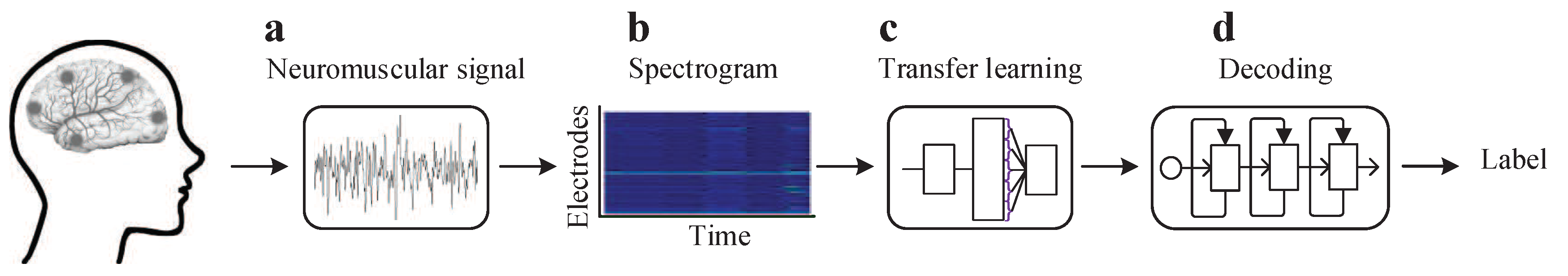
:1. Introduction
2. Silent Speech Data
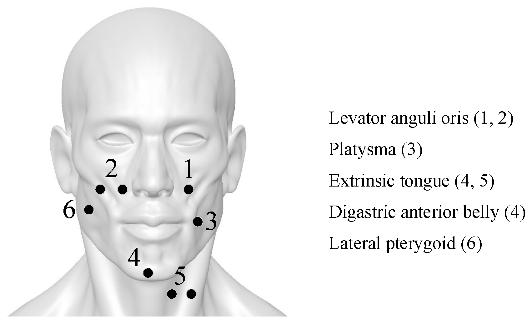
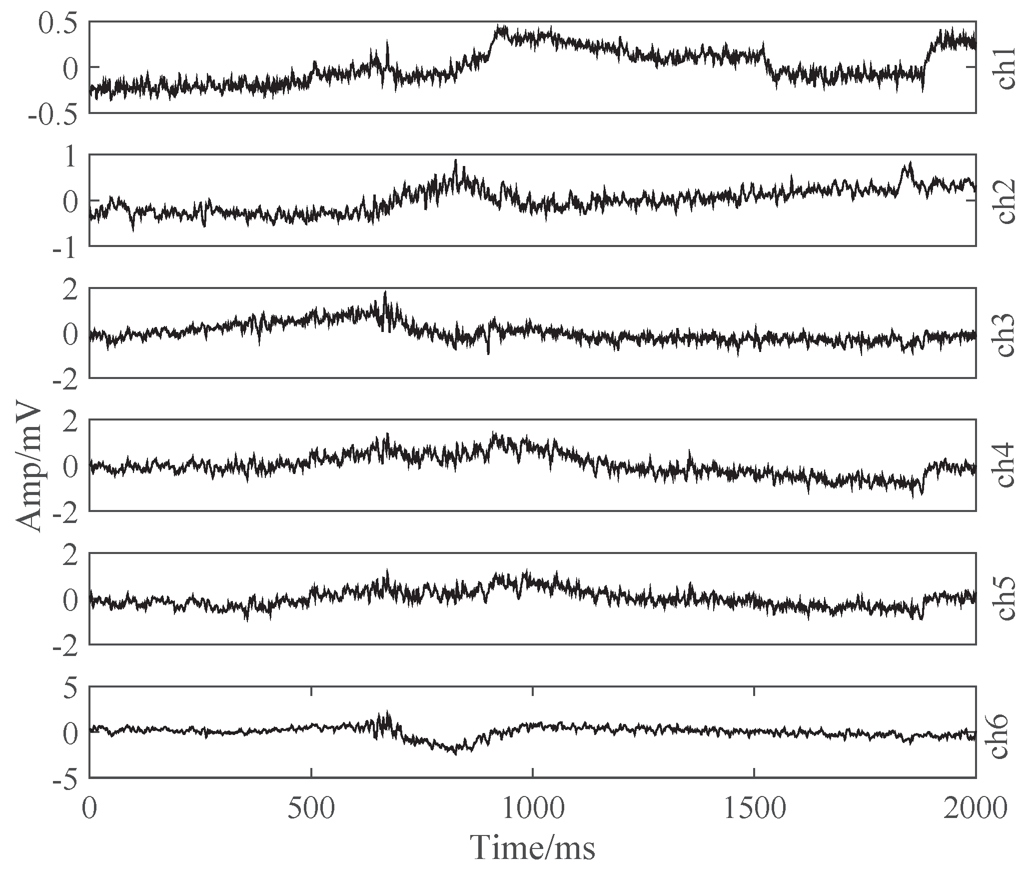
2.1. Capturing Speech-Related sEMG
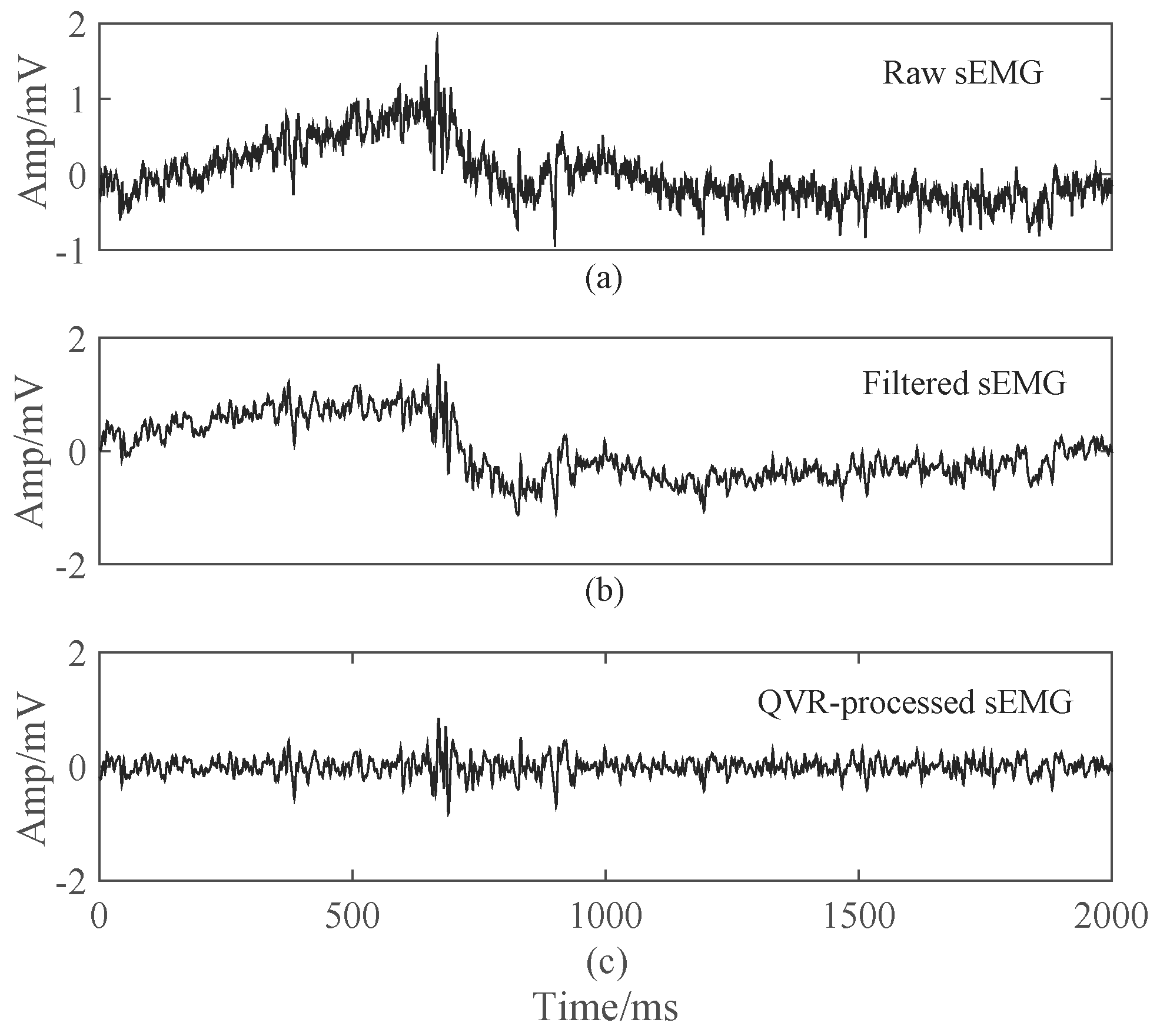
2.2. Preprocessing
3. Processing Methods
3.1. Spectrogram Images
3.2. Feature Extraction
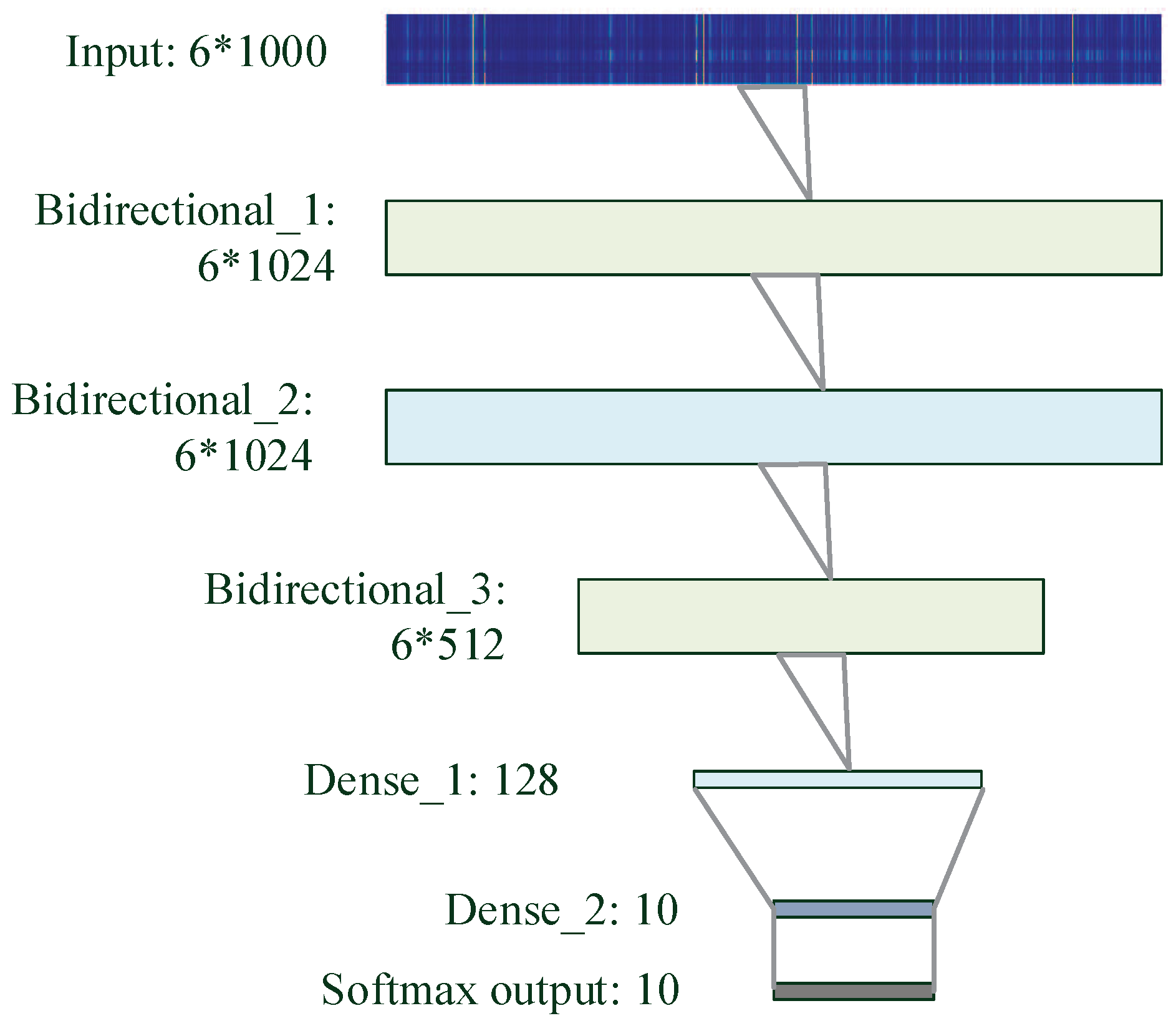
3.3. Decoder Design
3.3.1. MLP
3.3.2. CNN
3.3.3. bLSTM
4. Results
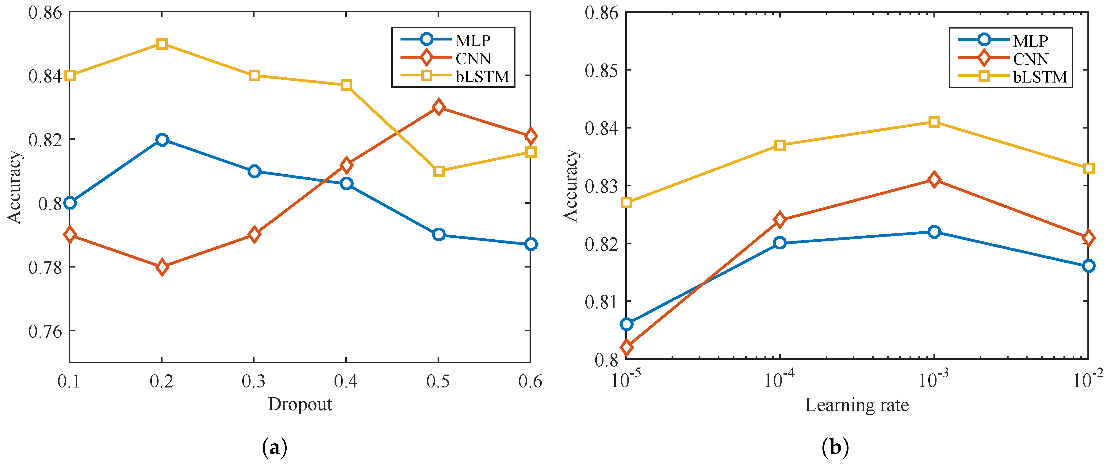
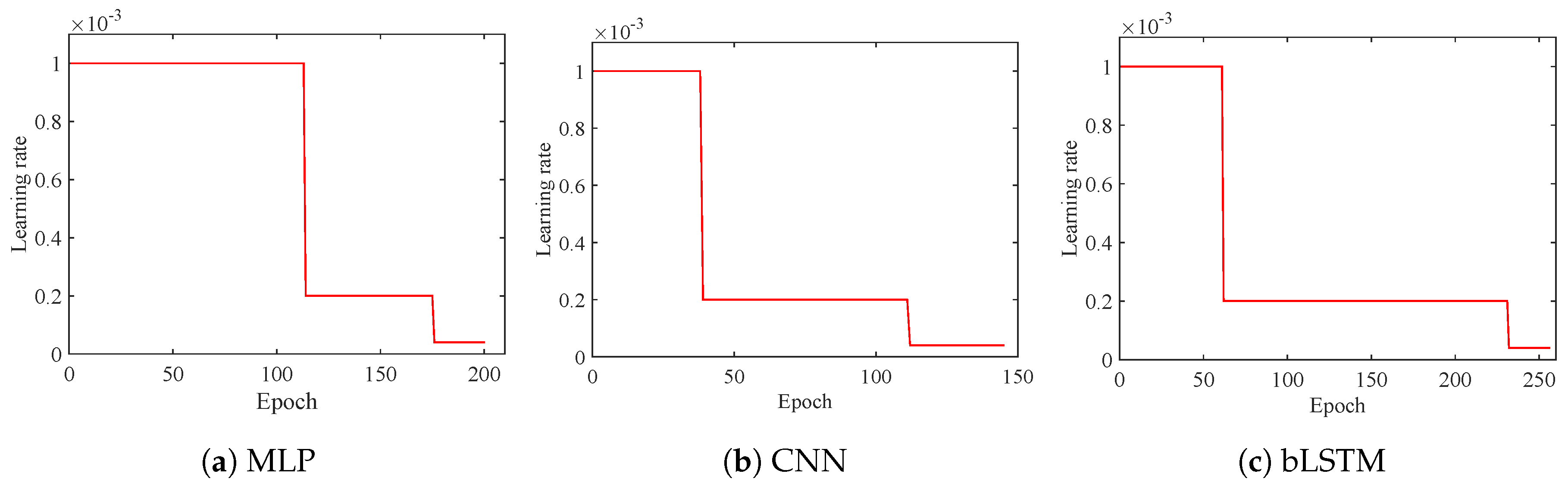
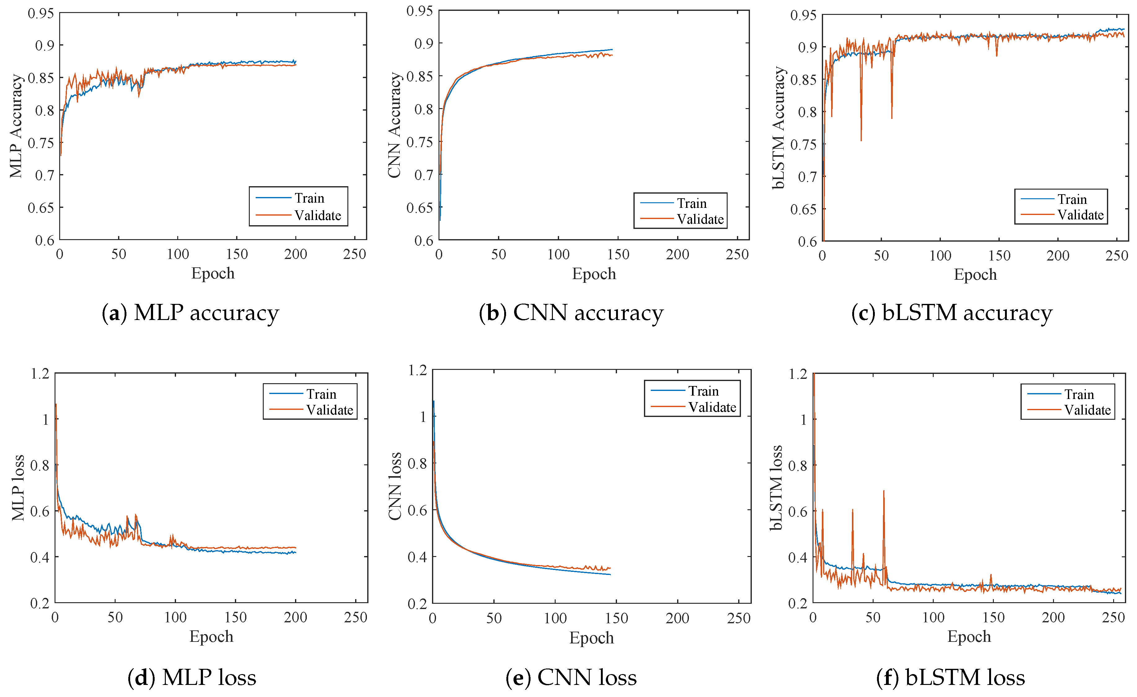
4.1. Decoder Optimization
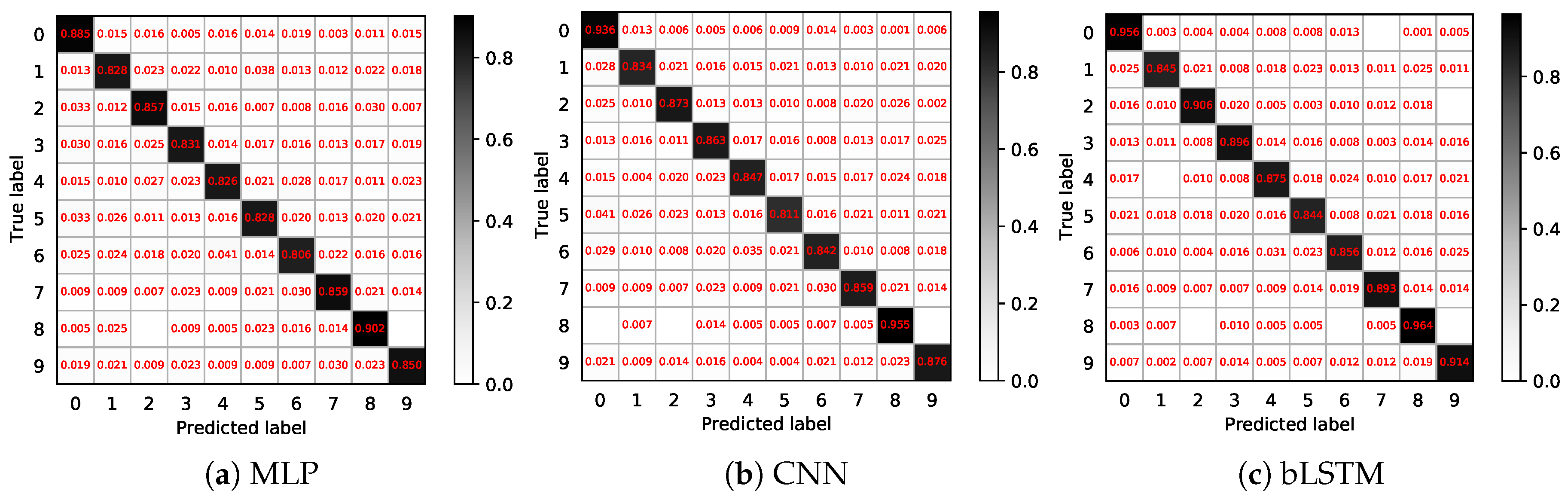
4.2. Decoding Results
5. Discussion
6. Conclusions
Author Contributions
Funding
Acknowledgments
Conflicts of Interest
References
- Vidal, J.J. Toward direct brain-computer communication. Annu. Rev. Biophys. Bioeng. 1973, 2, 157–180. [Google Scholar] [CrossRef] [PubMed]
- Pfurtscheller, G.; Flotzinger, D.; Kalcher, J. Brain-computer interface-a new communication device for handicapped persons. J. Microcomp. Appl. 1993, 16, 293–299. [Google Scholar] [CrossRef]
- Ang, K.K.; Chua, K.S.G.; Phua, K.S.; Wang, C.; Chin, Z.Y.; Kuah, C.W.K.; Low, W.; Guan, C. A randomized controlled trial of EEG-based motor imagery brain-computer interface robotic rehabilitation for stroke. Clin. EEG Neurosci. 2015, 46, 310–320. [Google Scholar] [CrossRef] [PubMed]
- Mahmood, M.; Mzurikwao, D.; Kim, Y.S.; Lee, Y.; Mishra, S.; Herbert, R.; Duarte, A.; Ang, C.S.; Yeo, W.H. Fully portable and wireless universal brain–machine interfaces enabled by flexible scalp electronics and deep learning algorithm. Nat. Mach. Intell. 2019, 1, 412–422. [Google Scholar] [CrossRef] [Green Version]
- Ramadan, R.A.; Vasilakos, A.V. Brain computer interface: Control signals review. Neurocomputing 2017, 223, 26–44. [Google Scholar] [CrossRef]
- Kapur, A.; Kapur, S.; Maes, P. Alterego: A personalized wearable silent speech interface. In 23rd International Conference on Intelligent User Interfaces; ACM: New York, NY, USA, 2018; pp. 43–53. [Google Scholar]
- Yau, W.C.; Arjunan, S.P.; Kumar, D.K. Classification of voiceless speech using facial muscle activity and vision based techniques. In Proceedings of the TENCON 2008-2008 IEEE Region 10 Conference, Hyderabad, India, 19–21 November 2008; IEEE: Piscataway, NJ, USA, 2008; pp. 1–6. [Google Scholar]
- Schultz, T.; Wand, M. Modeling coarticulation in EMG-based continuous speech recognition. Speech Commun. 2010, 52, 341–353. [Google Scholar] [CrossRef] [Green Version]
- Wand, M.; Janke, M.; Schultz, T. Tackling speaking mode varieties in EMG-based speech recognition. IEEE Trans. Biomed. Eng. 2014, 61, 2515–2526. [Google Scholar] [CrossRef]
- Wand, M.; Schultz, T. Speaker-adaptive speech recognition based on surface electromyography. In International Joint Conference on Biomedical Engineering Systems and Technologies; Springer: Berlin/Heidelberg, Germany, 2009; pp. 271–285. [Google Scholar]
- Deng, Y.; Colby, G.; Heaton, J.T.; Meltzner, G.S. Signal processing advances for the MUTE sEMG-based silent speech recognition system. In Proceedings of the MILCOM 2012-2012 IEEE Military Communications Conference, Orlando, FL, USA, 29 October–1 November 2012; IEEE: Piscataway, NJ, USA, 2012; pp. 1–6. [Google Scholar]
- Soon, M.W.; Anuar, M.I.H.; Abidin, M.H.Z.; Azaman, A.S.; Noor, N.M. Speech recognition using facial sEMG. In Proceedings of the 2017 IEEE International Conference on Signal and Image Processing Applications (ICSIPA), Kuching, Malaysia, 12–14 September 2017; IEEE: Piscataway, NJ, USA, 2017; pp. 1–5. [Google Scholar]
- Denby, B.; Schultz, T.; Honda, K.; Hueber, T.; Gilbert, J.M.; Brumberg, J.S. Silent speech interfaces. Speech Commun. 2010, 52, 270–287. [Google Scholar] [CrossRef] [Green Version]
- Hofe, R.; Ell, S.R.; Fagan, M.J.; Gilbert, J.M.; Green, P.D.; Moore, R.K.; Rybchenko, S.I. Small-vocabulary speech recognition using a silent speech interface based on magnetic sensing. Speech Commun. 2013, 55, 22–32. [Google Scholar] [CrossRef]
- Sugie, N.; Tsunoda, K. A speech prosthesis employing a speech synthesizer-vowel discrimination from perioral muscle activities and vowel production. IEEE Trans. Biomed. Eng. 1985, BME-32, 485–490. [Google Scholar] [CrossRef] [PubMed]
- Morse, M.S.; O’Brien, E.M. Research summary of a scheme to ascertain the availability of speech information in the myoelectric signals of neck and head muscles using surface electrodes. Comput. Biol. Med. 1986, 16, 399–410. [Google Scholar] [CrossRef]
- Morse, M.S.; Day, S.H.; Trull, B.; Morse, H. Use of myoelectric signals to recognize speech. In Images of the Twenty-First Century, Proceedings of the Annual International Engineering in Medicine and Biology Society, Seattle, WA, USA, 9–12 November 1989; IEEE: Piscataway, NJ, USA, 1989; pp. 1793–1794. [Google Scholar]
- Morse, M.; Gopalan, Y.; Wright, M. Speech recognition using myoelectric signals with neural networks. In Proceedings of the Annual International Conference of the IEEE Engineering in Medicine and Biology Society, Orlando, FL, USA, 31 October–3 November 1991; IEEE: Piscataway, NJ, USA, 1991; Volume 13, pp. 1877–1878. [Google Scholar]
- Chan, A.D.; Englehart, K.; Hudgins, B.; Lovely, D.F. Myo-electric signals to augment speech recognition. Med. Biol. Eng. Comput. 2001, 39, 500–504. [Google Scholar] [CrossRef] [PubMed]
- Jorgensen, C.; Lee, D.D.; Agabont, S. Sub auditory speech recognition based on EMG signals. In Proceedings of the International Joint Conference on Neural Networks, 2003, Portland, OR, USA, 20–24 July 2003; IEEE: Piscataway, NJ, USA, 2003; Volume 4, pp. 3128–3133. [Google Scholar]
- Jou, S.C.; Schultz, T.; Walliczek, M.; Kraft, F.; Waibel, A. Towards continuous speech recognition using surface electromyography. In Proceedings of the Ninth International Conference on Spoken Language Processing, Pittsburgh, PA, USA, 17–21 September 2006; pp. 573–576. [Google Scholar]
- Meltzner, G.S.; Heaton, J.T.; Deng, Y.; De Luca, G.; Roy, S.H.; Kline, J.C. Development of sEMG sensors and algorithms for silent speech recognition. J. Neural Eng. 2018, 15, 046031. [Google Scholar] [CrossRef] [PubMed]
- Martini, F.; Nath, J.L.; Bartholomew, E.F.; Ober, W.C.; Ober, C.E.; Welch, K.; Hutchings, R.T. Fundamentals of Anatomy & Physiology; Pearson Benjamin Cummings: San Francisco, CA, USA, 2006; Volume 7. [Google Scholar]
- Marieb, E.N.; Hoehn, K. Human Anatomy & Physiology, 9th ed.; Pearson: London, UK, 2013; pp. 276–482. [Google Scholar]
- Schultz, T.; Wand, M.; Hueber, T.; Krusienski, D.J.; Herff, C.; Brumberg, J.S. Biosignal-Based Spoken Communication: A Survey. IEEE Trans. Audio. Speech. Lang. Process. 2017, 25, 2257–2271. [Google Scholar] [CrossRef]
- Chollet, F. Xception: Deep learning with depthwise separable convolutions. In Proceedings of the IEEE Conference on Computer Vision and Pattern Recognition, Honolulu, HI, USA, 21–26 July 2017; IEEE: NewYork, NY, USA, 2017; pp. 1251–1258. [Google Scholar]
- Jinsakul, N.; Tsai, C.F.; Tsai, C.E.; Wu, P. Enhancement of Deep Learning in Image Classification Performance Using Xception with the Swish Activation Function for Colorectal Polyp Preliminary Screening. Mathematics 2019, 7, 1170. [Google Scholar] [CrossRef] [Green Version]
- Yang, L.; Chen, X.; Tao, L. Acoustic scene classification using multi-scale features. In Proceedings of the Workshop on DCASE 2018, Surrey, UK, 19–20 November 2018. [Google Scholar]
- Yang, L.; Yang, P.; Ni, R.; Zhao, Y. Xception-Based General Forensic Method on Small-Size Images. In Advances in Intelligent Information Hiding and Multimedia Signal Processing; Springer: Berlin, Germany, 2020; pp. 361–369. [Google Scholar]
- Hermens, H.J.; Freriks, B.; Disselhorstklug, C.; Rau, G. Development of recommendations for SEMG sensors and sensor placement procedures. J. Electromyogr. Kinesiol. 2000, 10, 361–374. [Google Scholar] [CrossRef]
- Roberts, A. Human Anatomy: The Definitive Visual Guide; Dorling Kindersley Ltd.: London, UK, 2016; pp. 50–65. [Google Scholar]
- Kenneth, S.S. Anatomy & Physiology: The Unity of Form and Function; McGraw-Hill: New York, NY, USA, 2017; pp. 307–570. [Google Scholar]
- Zhang, M.; Wang, Y.; Wei, Z.; Yang, M.; Luo, Z.; Li, G. Inductive conformal prediction for silent speech recognition. J. Neural Eng. 2020, in press. [Google Scholar] [CrossRef]
- Maier-Hein, L.; Metze, F.; Schultz, T.; Waibel, A. Session independent non-audible speech recognition using surface electromyography. In Proceedings of the IEEE Workshop on Automatic Speech Recognition and Understanding, 2005, San Juan, Puerto Rico, 27 November–1 December 2005; IEEE: Piscataway, NJ, USA, 2005; pp. 331–336. [Google Scholar]
- Stepp, C.E.; Heaton, J.T.; Rolland, R.G.; Hillman, R.E. Neck and face surface electromyography for prosthetic voice control after total laryngectomy. IEEE Trans. Neural Syst. Rehabil. Eng. 2009, 17, 146–155. [Google Scholar] [CrossRef]
- Hakonen, M.; Piitulainen, H.; Visala, A. Current state of digital signal processing in myoelectric interfaces and related applications. Biomed. Signal Process. Control 2015, 18, 334–359. [Google Scholar] [CrossRef] [Green Version]
- Fasano, A.; Villani, V. Baseline wander removal for bioelectrical signals by quadratic variation reduction. Signal Process. 2014, 99, 48–57. [Google Scholar] [CrossRef]
- Sairamya, N.; Susmitha, L.; George, S.T.; Subathra, M. Hybrid Approach for Classification of Electroencephalographic Signals Using Time–Frequency Images With Wavelets and Texture Features. In Intelligent Data Analysis for Biomedical Applications; Elsevier: Amsterdam, The Netherlands, 2019; pp. 253–273. [Google Scholar]
- Huang, J.; Chen, B.; Yao, B.; He, W. ECG Arrhythmia Classification Using STFT-Based Spectrogram and Convolutional Neural Network. IEEE Access 2019, 7, 92871–92880. [Google Scholar] [CrossRef]
- Pandey, A.; Wang, D. Exploring Deep Complex Networks for Complex Spectrogram Enhancement. In Proceedings of the ICASSP 2019-2019 IEEE International Conference on Acoustics, Speech and Signal Processing (ICASSP), Brighton, UK, 12–17 May 2019; IEEE: Piscataway, NJ, USA, 2019; pp. 6885–6889. [Google Scholar]
- Géron, A. Hands-on Machine Learning with Scikit-Learn and TensorFlow: Concepts, Tools, and Techniques to Build Intelligent Systems; O’Reilly Media, Inc.: Sebastopol, CA, USA, 2017. [Google Scholar]
- Xianshun, C. Keras Implementation of Video Classifier. Available online: https://github.com/chen0040/keras-video-classifier (accessed on 13 April 2018).
- Anumanchipalli, G.K.; Chartier, J.; Chang, E.F. Speech synthesis from neural decoding of spoken sentences. Nature 2019, 568, 493. [Google Scholar] [CrossRef] [PubMed]
- Orhan, U.; Hekim, M.; Ozer, M. EEG signals classification using the K-means clustering and a multilayer perceptron neural network model. Expert Syst. Appl. 2011, 38, 13475–13481. [Google Scholar] [CrossRef]
- Tang, J.; Deng, C.; Huang, G.B. Extreme learning machine for multilayer perceptron. IEEE Trans. Neural Netw. Learn. Syst. 2015, 27, 809–821. [Google Scholar] [CrossRef]
- Srivastava, N.; Hinton, G.; Krizhevsky, A.; Sutskever, I.; Salakhutdinov, R. Dropout: A simple way to prevent neural networks from overfitting. J. Mach. Learn. Res. 2014, 15, 1929–1958. [Google Scholar]
- Shin, H.C.; Roth, H.R.; Gao, M.; Lu, L.; Xu, Z.; Nogues, I.; Yao, J.; Mollura, D.; Summers, R.M. Deep convolutional neural networks for computer-aided detection: CNN architectures, dataset characteristics and transfer learning. IEEE Trans. Med. Imag. 2016, 35, 1285–1298. [Google Scholar] [CrossRef] [Green Version]
- Wang, J.; Yang, Y.; Mao, J.; Huang, Z.; Huang, C.; Xu, W. Cnn-rnn: A unified framework for multi-label image classification. In Proceedings of the IEEE Conference on Computer Vision and Pattern Recognition, Las Vegas, NV, USA, 27–30 June 2016; IEEE: Piscataway, NJ, USA, 2016; pp. 2285–2294. [Google Scholar]
- Goodfellow, I.; Bengio, Y.; Courville, A. Deep learning; MIT Press: Cambridge, MA, USA, 2016. [Google Scholar]
- Bjorck, N.; Gomes, C.P.; Selman, B.; Weinberger, K.Q. Understanding batch normalization. In Proceedings of the Advances in Neural Information Processing Systems, Montreal, QC, Canada, 3–8 December 2018; Curran Associates, Inc.: Red Hook, NY, USA, 2018; pp. 7694–7705. [Google Scholar]
- Ioffe, S.; Szegedy, C. Batch normalization: Accelerating deep network training by reducing internal covariate shift. arXiv 2015, arXiv:1502.03167. [Google Scholar]
- Santurkar, S.; Tsipras, D.; Ilyas, A.; Madry, A. How does batch normalization help optimization? In Proceedings of the Advances in Neural Information Processing Systems, Montreal, QC, Canada, 3–8 December 2018; Curran Associates, Inc.: Red Hook, NY, USA, 2018; pp. 2483–2493. [Google Scholar]
- Cho, K.; Van Merriënboer, B.; Gulcehre, C.; Bahdanau, D.; Bougares, F.; Schwenk, H.; Bengio, Y. Learning phrase representations using RNN encoder-decoder for statistical machine translation. arXiv 2014, arXiv:1406.1078. [Google Scholar]
- Sak, H.; Senior, A.; Beaufays, F. Long short-term memory based recurrent neural network architectures for large vocabulary speech recognition. arXiv 2014, arXiv:1402.1128. [Google Scholar]
- Zeiler, M.D. Adadelta: An adaptive learning rate method. arXiv 2012, arXiv:1212.5701. [Google Scholar]
- Yu, C.; Qi, X.; Ma, H.; He, X.; Wang, C.; Zhao, Y. LLR: Learning learning rates by LSTM for training neural networks. Neurocomputing 2020, 394, 41–50. [Google Scholar] [CrossRef]
- Janke, M.; Diener, L. Emg-to-speech: Direct generation of speech from facial electromyographic signals. IEEE Trans. Audio. Speech. Lang. Process. 2017, 25, 2375–2385. [Google Scholar] [CrossRef] [Green Version]
- Denby, B.; Chen, S.; Zheng, Y.; Xu, K.; Yin, Y.; Leboullenger, C.; Roussel, P. Recent results in silent speech interfaces. J. Acoust. Soc. Am. 2017, 141, 3646. [Google Scholar] [CrossRef]
- Cler, M.J.; Nieto-Castanon, A.; Guenther, F.H.; Stepp, C.E. Surface electromyographic control of speech synthesis. In Proceedings of the 2014 36th Annual International Conference of the IEEE Engineering in Medicine and Biology Society, Chicago, IL, USA, 26–30 August 2014; IEEE: Piscataway, NJ, USA, 2014; pp. 5848–5851. [Google Scholar]


| Label | ‘0’ | ‘1’ | ‘2’ | ‘3’ | ‘4’ | ‘5’ | ‘6’ | ‘7’ | ‘8’ | ‘9’ |
| Word | ’噪’ | ’1#’ | ’2#’ | ’ 前’ | ’后’ | ’左’ | ’右’ | ’快’ | ’慢’ | ’停’ |
| Samples | 7964 | 6707 | 6814 | 6978 | 6593 | 6510 | 6682 | 6883 | 7614 | 6524 |
| Model | Optimizer | Dropout | Learning Rate | Activation | Batch Size |
|---|---|---|---|---|---|
| MLP | adam | 0.2 | 1 | ReLU | 32 |
| CNN | adadelta | 0.5 | 1 | ReLU | 32 |
| bLSTM | rmsprop | 0.2 | 1 | ReLU | 32 |
© 2020 by the authors. Licensee MDPI, Basel, Switzerland. This article is an open access article distributed under the terms and conditions of the Creative Commons Attribution (CC BY) license (http://creativecommons.org/licenses/by/4.0/).
Share and Cite
Wang, Y.; Zhang, M.; Wu, R.; Gao, H.; Yang, M.; Luo, Z.; Li, G. Silent Speech Decoding Using Spectrogram Features Based on Neuromuscular Activities. Brain Sci. 2020, 10, 442. https://doi.org/10.3390/brainsci10070442
Wang Y, Zhang M, Wu R, Gao H, Yang M, Luo Z, Li G. Silent Speech Decoding Using Spectrogram Features Based on Neuromuscular Activities. Brain Sciences. 2020; 10(7):442. https://doi.org/10.3390/brainsci10070442
Chicago/Turabian StyleWang, You, Ming Zhang, RuMeng Wu, Han Gao, Meng Yang, Zhiyuan Luo, and Guang Li. 2020. "Silent Speech Decoding Using Spectrogram Features Based on Neuromuscular Activities" Brain Sciences 10, no. 7: 442. https://doi.org/10.3390/brainsci10070442