Spatiotemporal Dynamics of Multiple Memory Systems During Category Learning

Abstract
:1. Introduction
2. fMRI Pilot Experiment
2.1. Materials and Methods
2.1.1. Participants
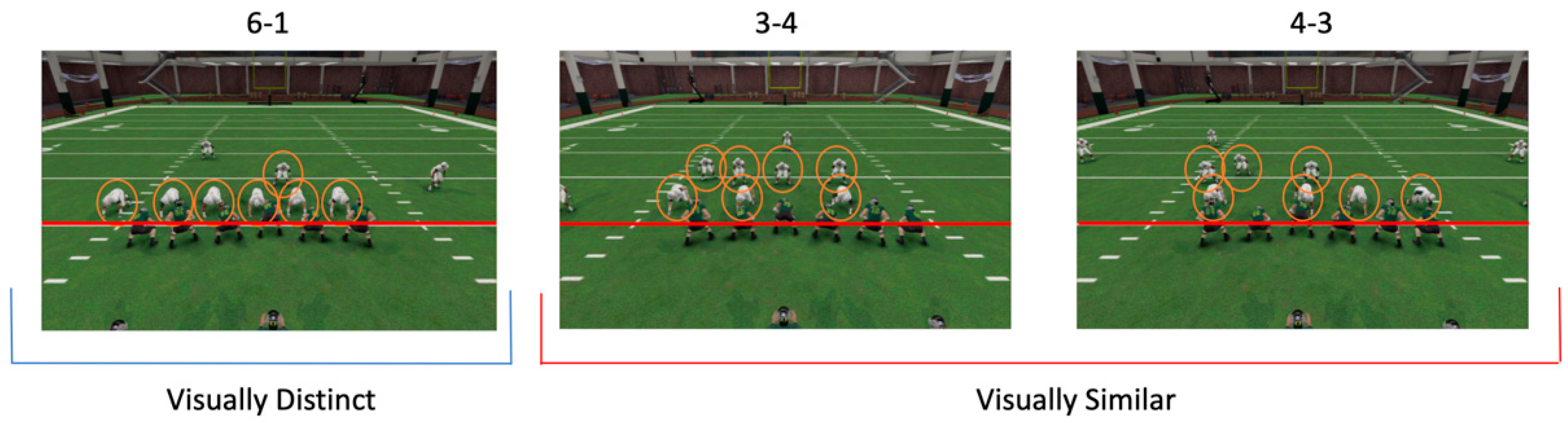
2.1.2. Task
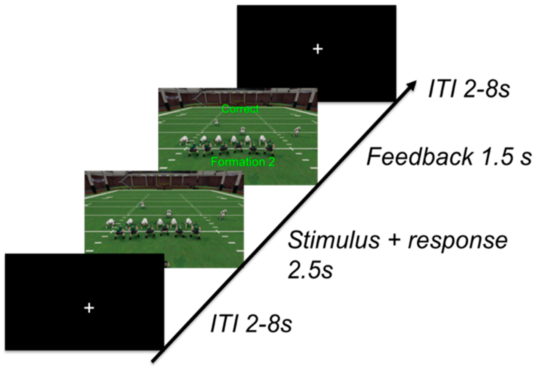
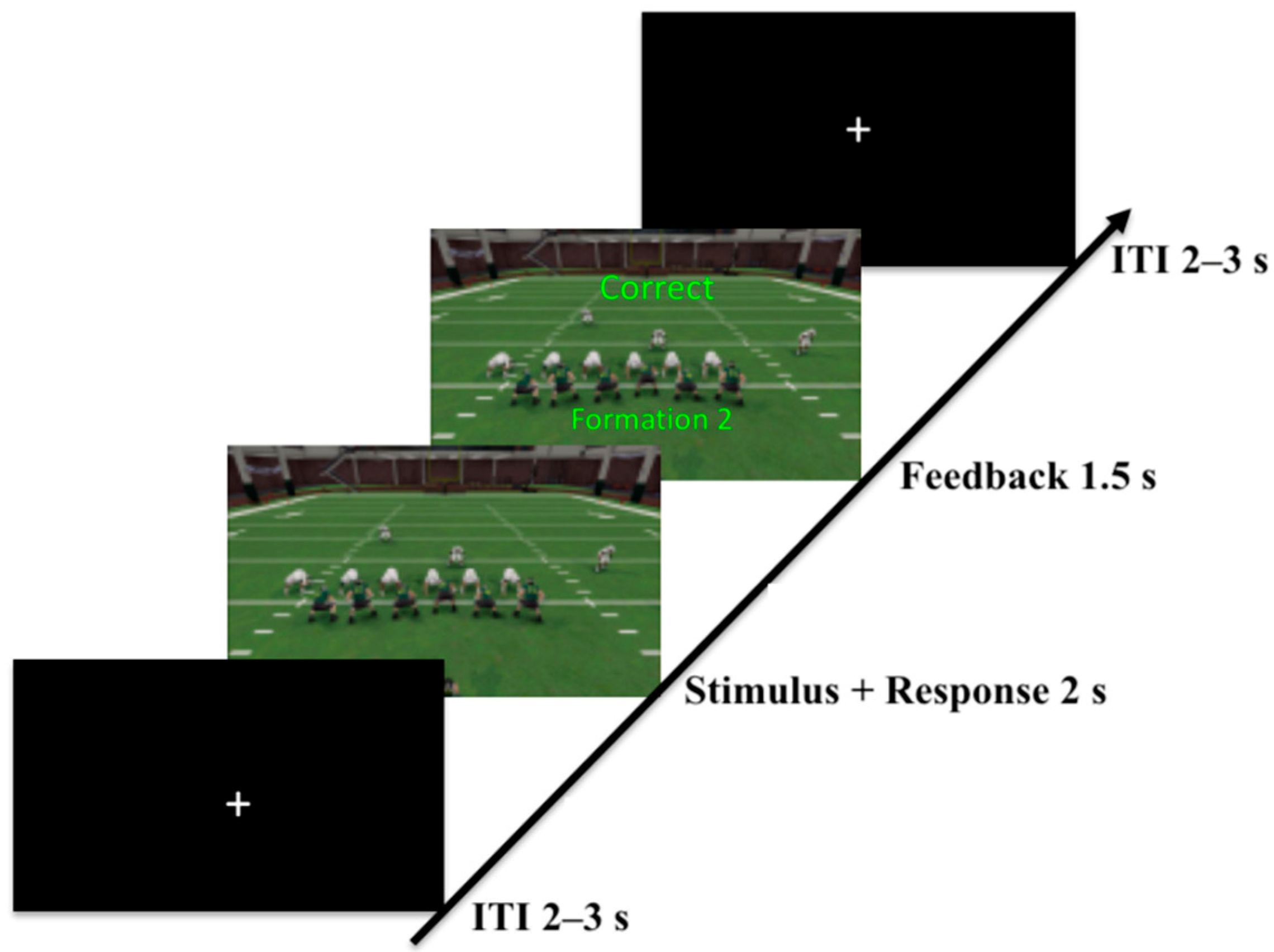
2.1.3. Procedure
2.1.4. fMRI Acquisition and Pre-Processing
2.2. Results
2.2.1. Behavioral Results
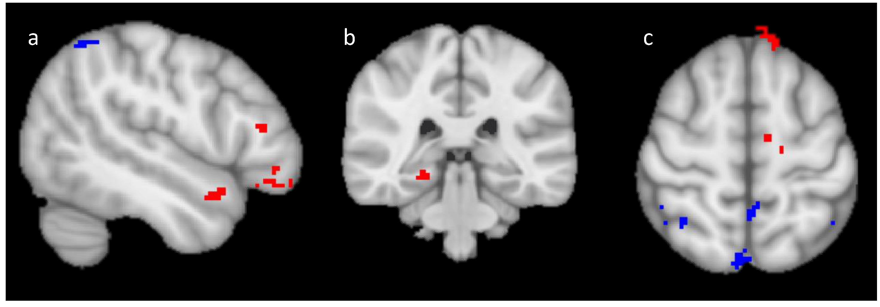
2.2.2. Univariate fMRI Analysis
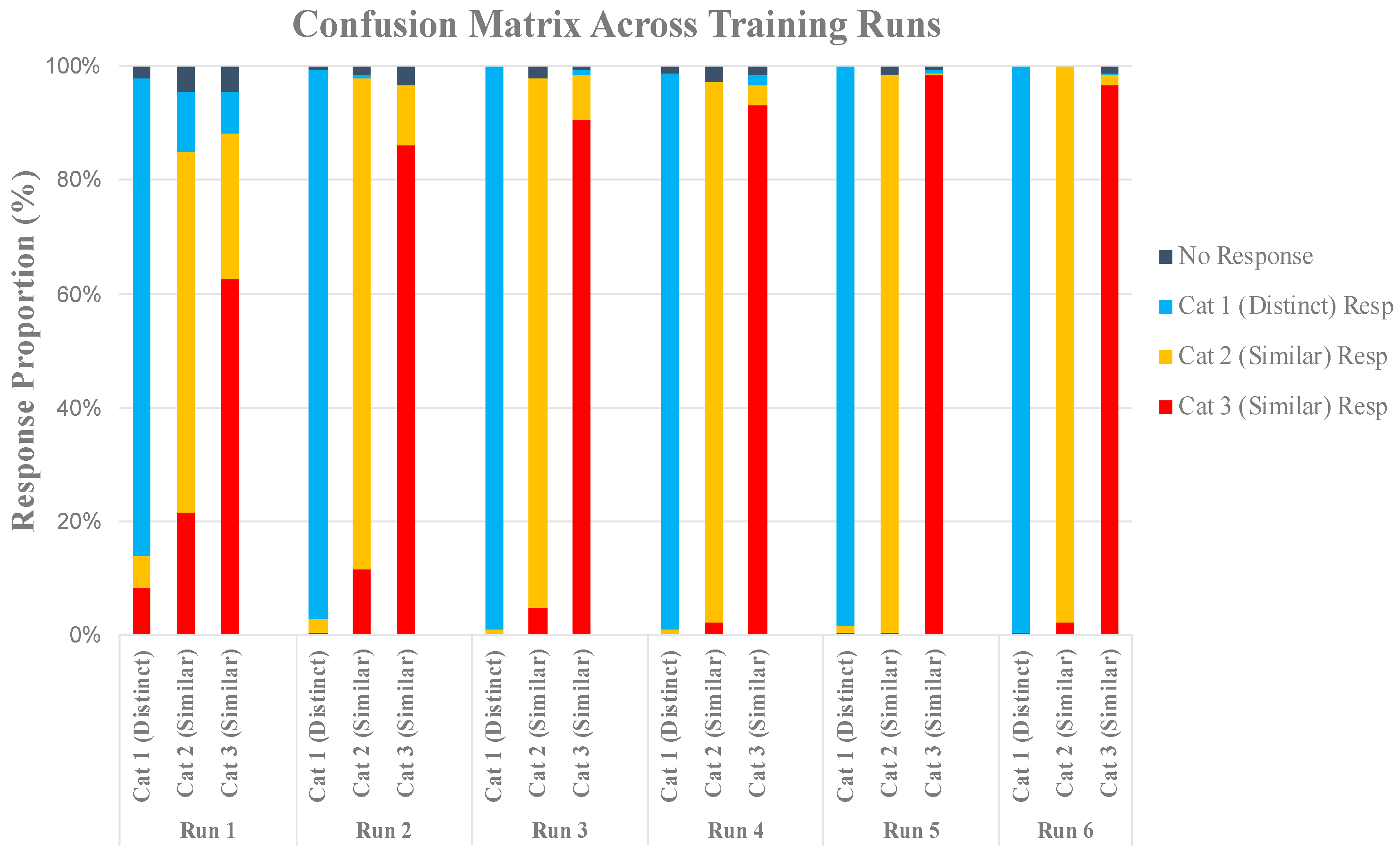
Training Analysis
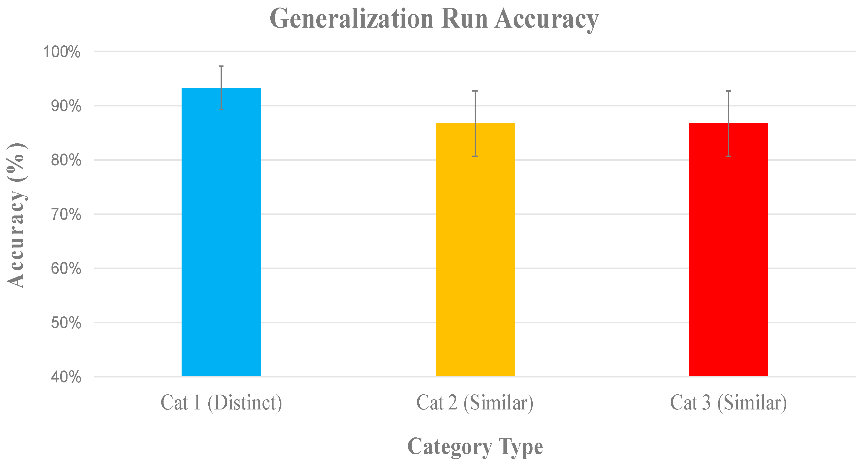
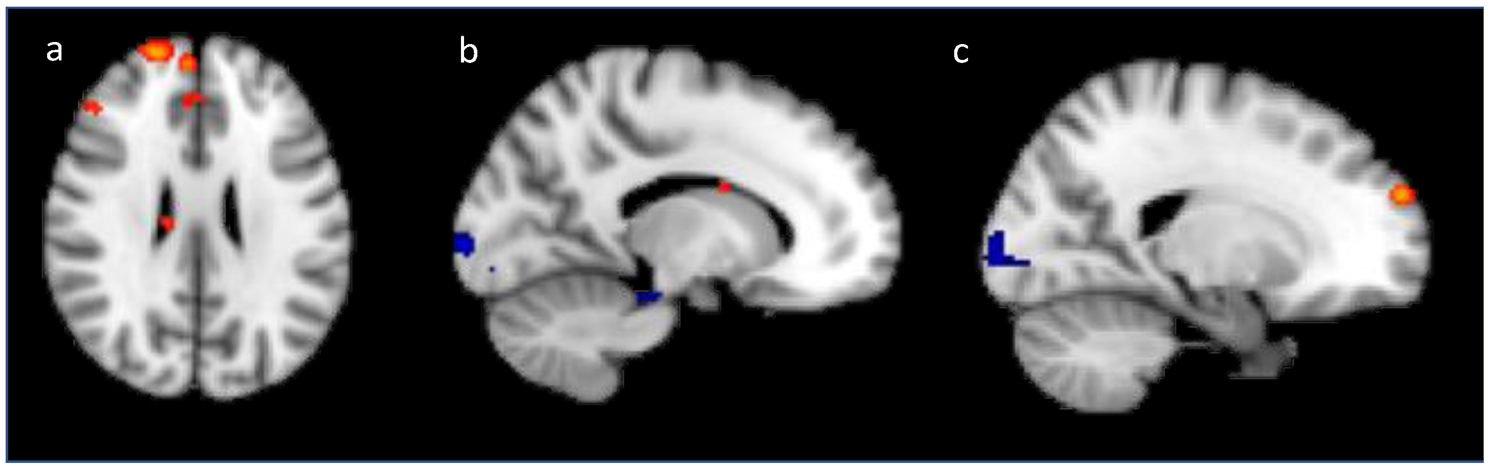
Generalization
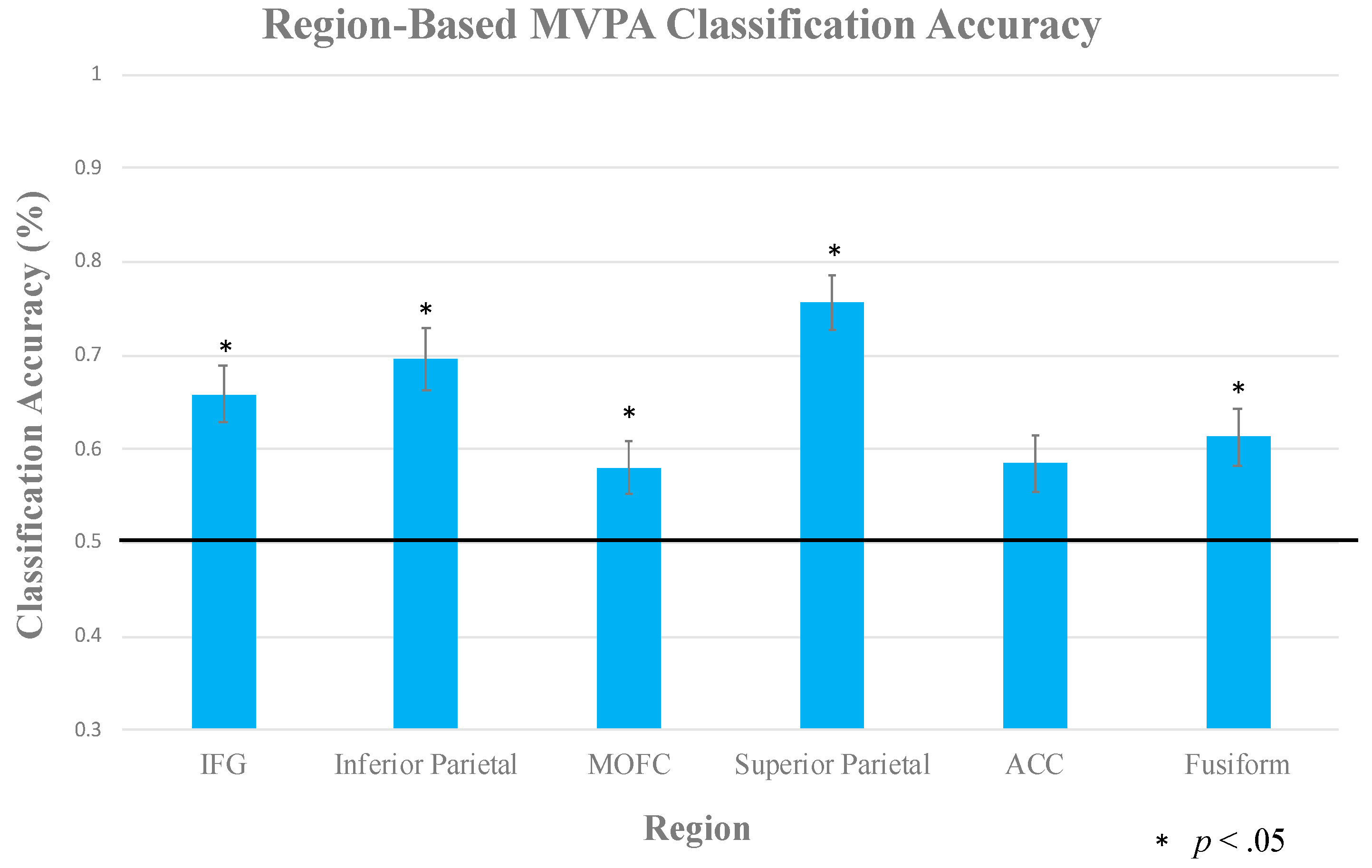
2.2.3. Multi-Voxel Pattern Analysis
3. dEEG Experiment
3.1. Materials and Methods
3.1.1. Participants
3.1.2. Task
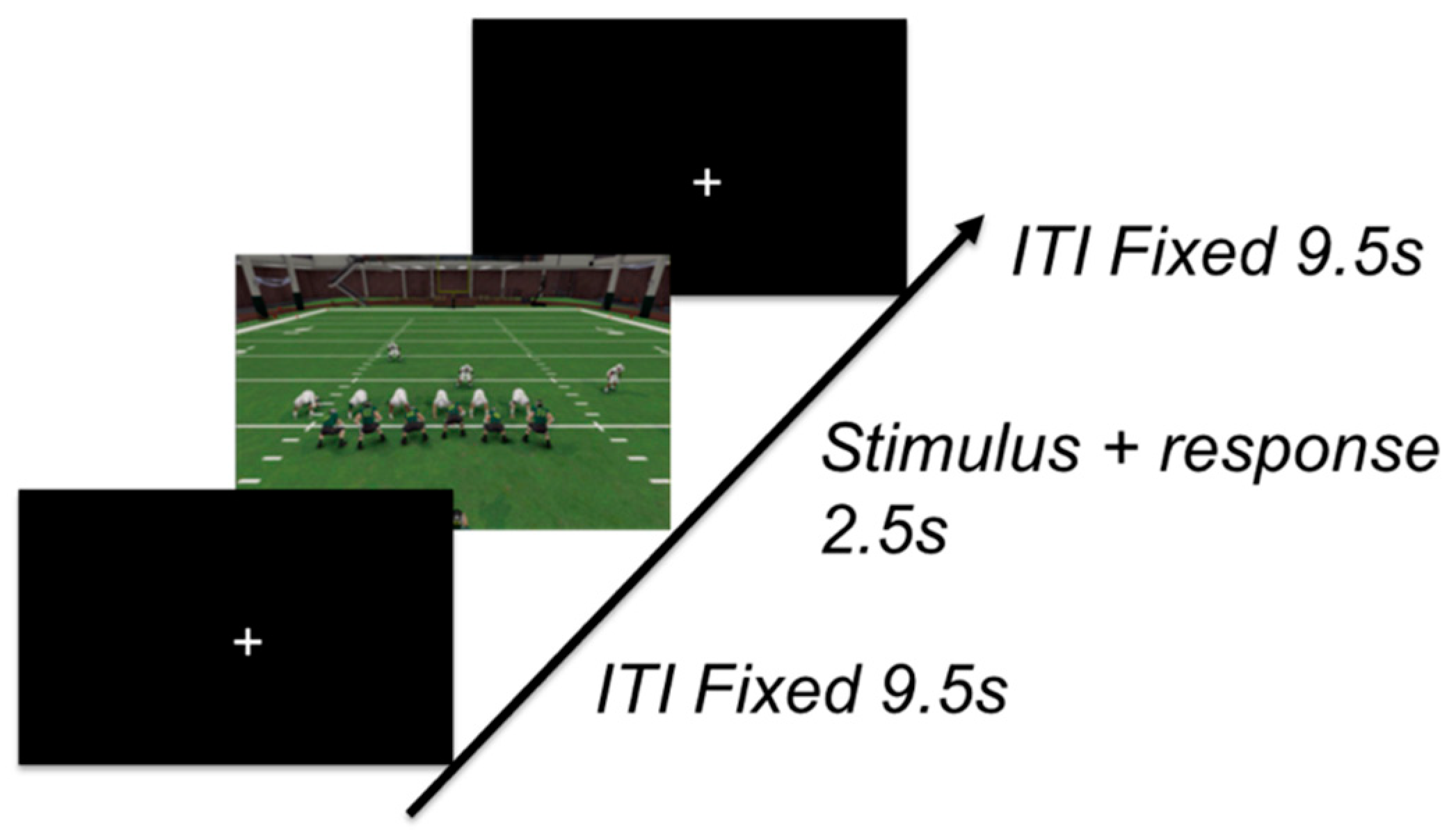
3.1.3. Procedure
3.1.4. Learning Criterion
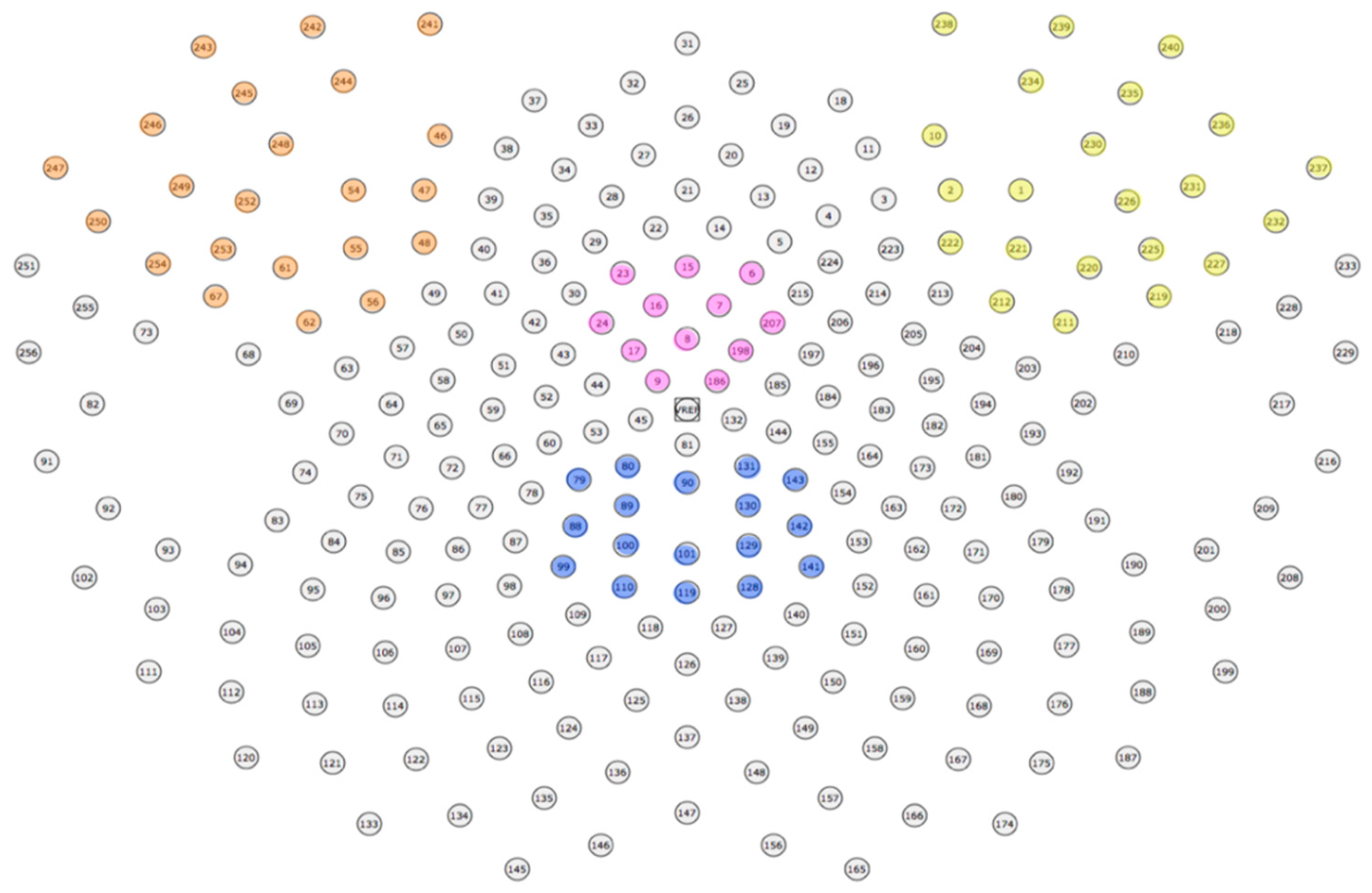
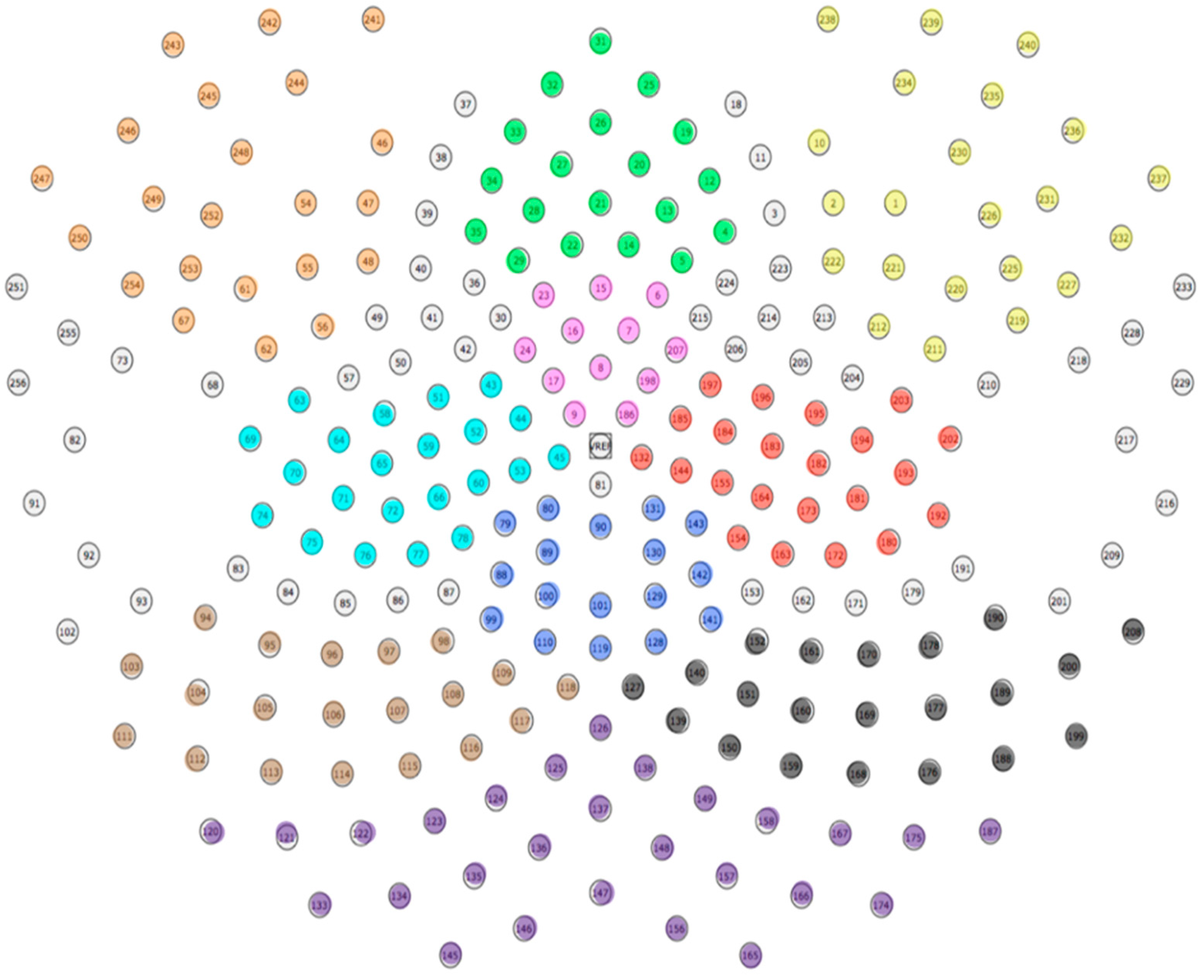
3.1.5. EEG Recording and Pre-Processing
3.2. Results
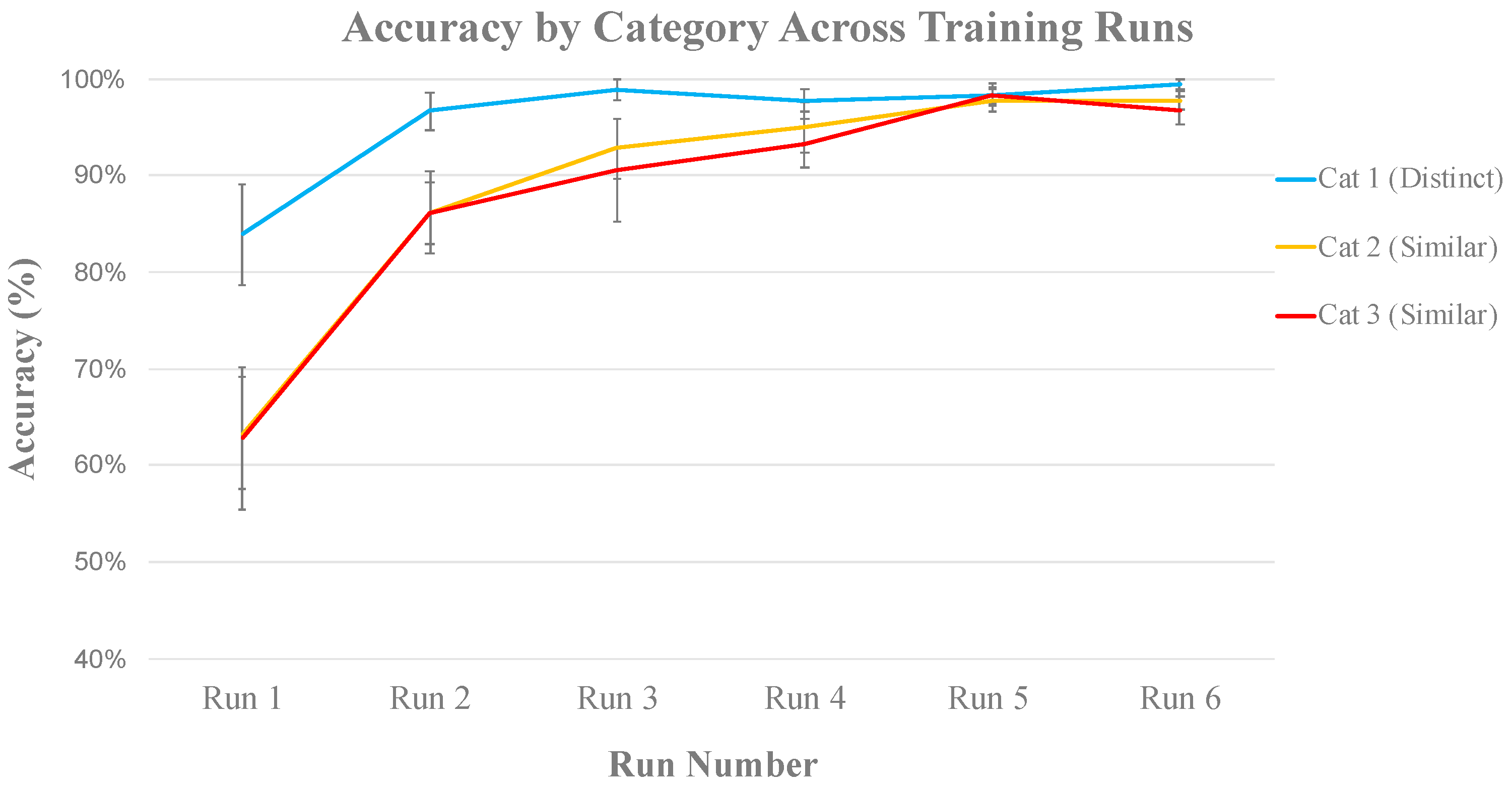
3.2.1. Behavioral Analysis
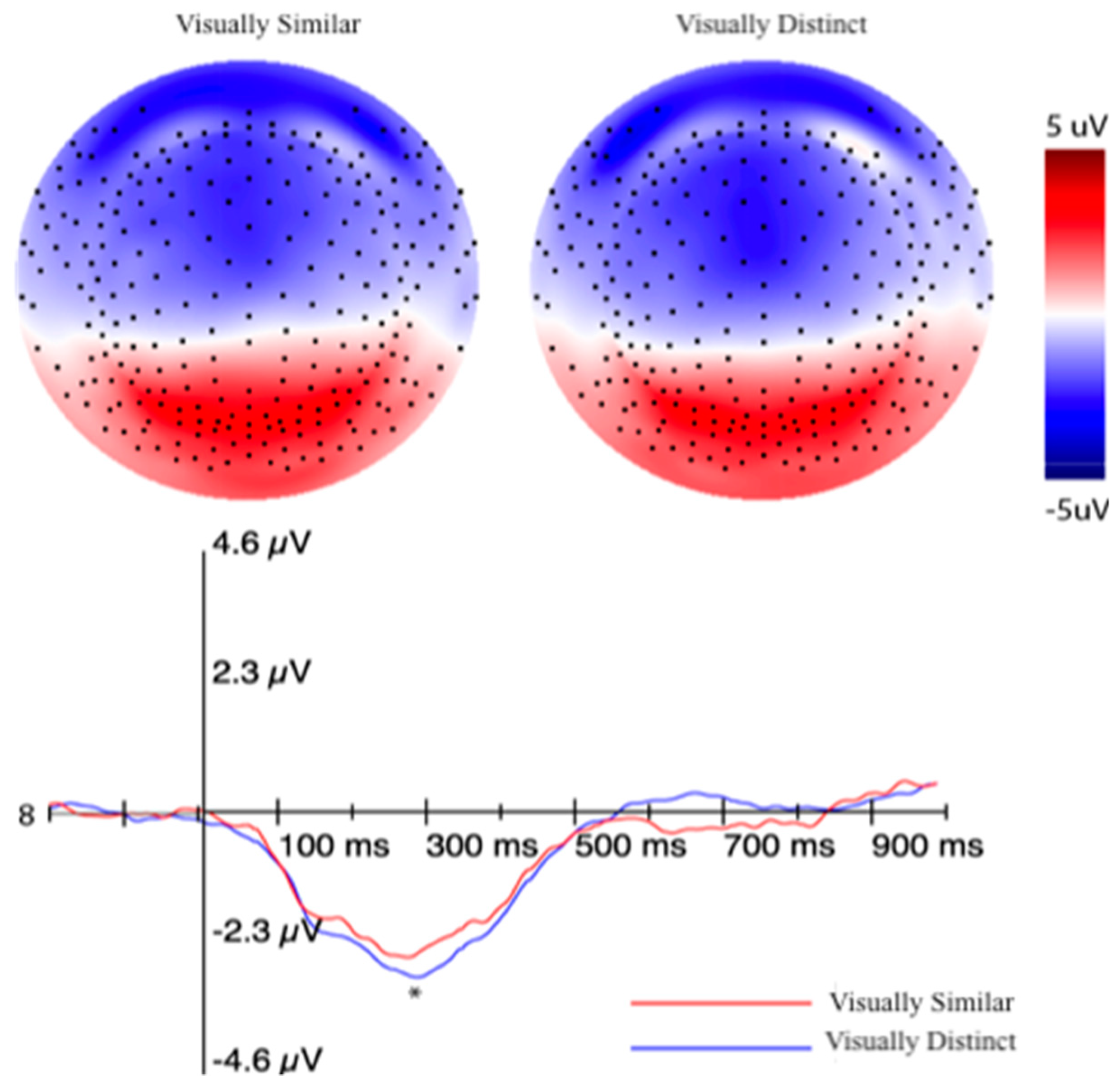
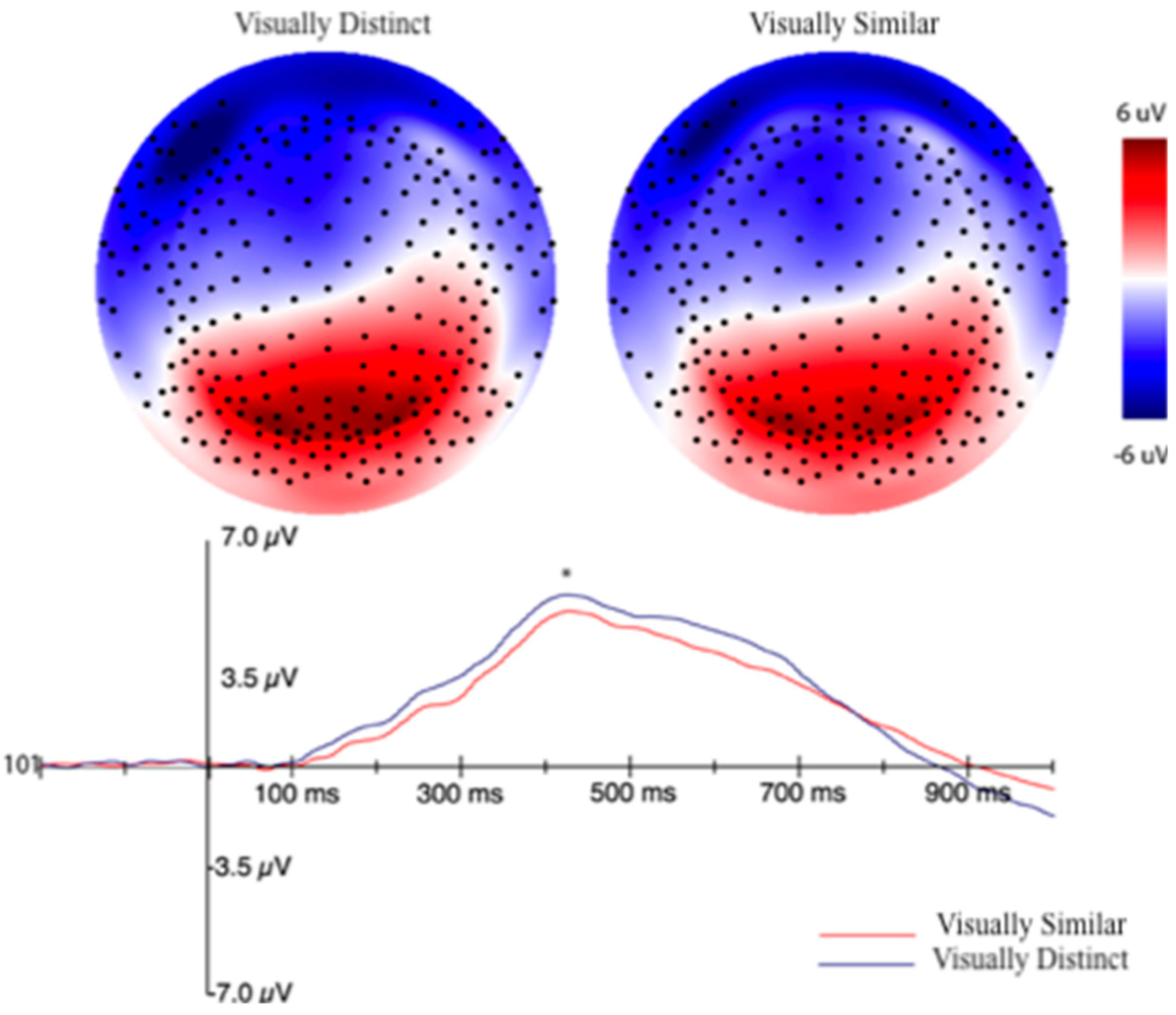
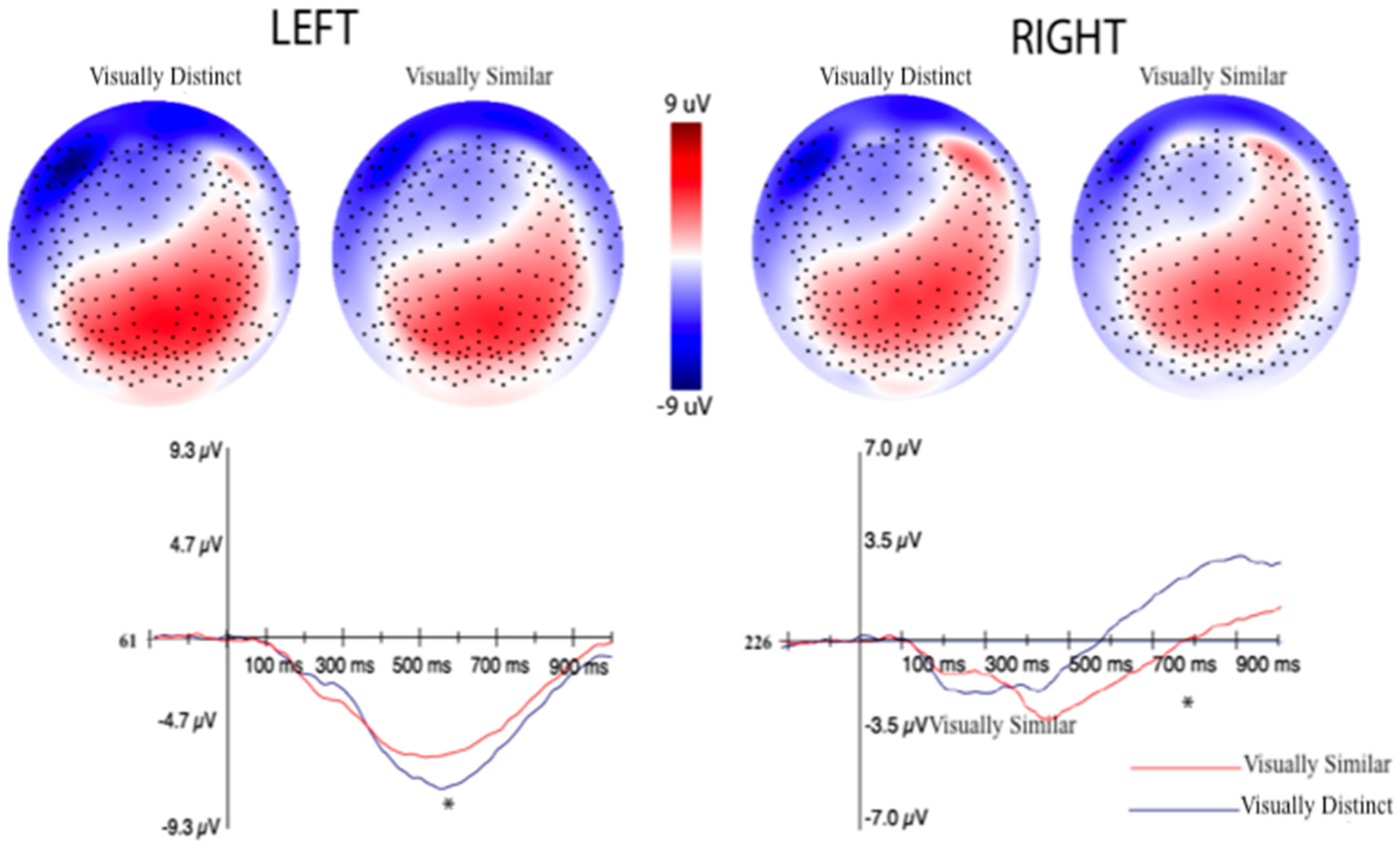
3.2.2. Event-Related Potentials (ERPs) Selection Motivation and Analysis
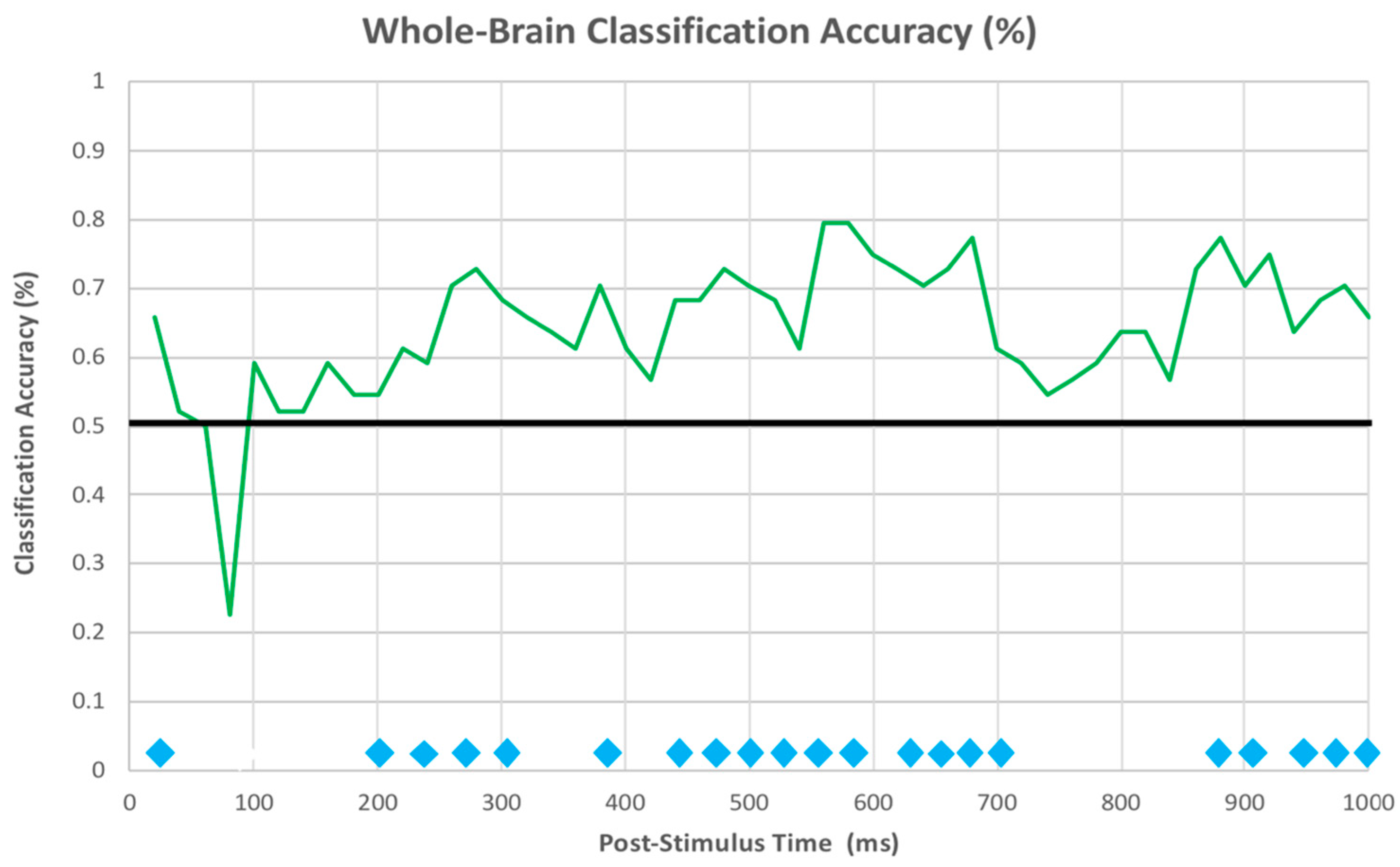
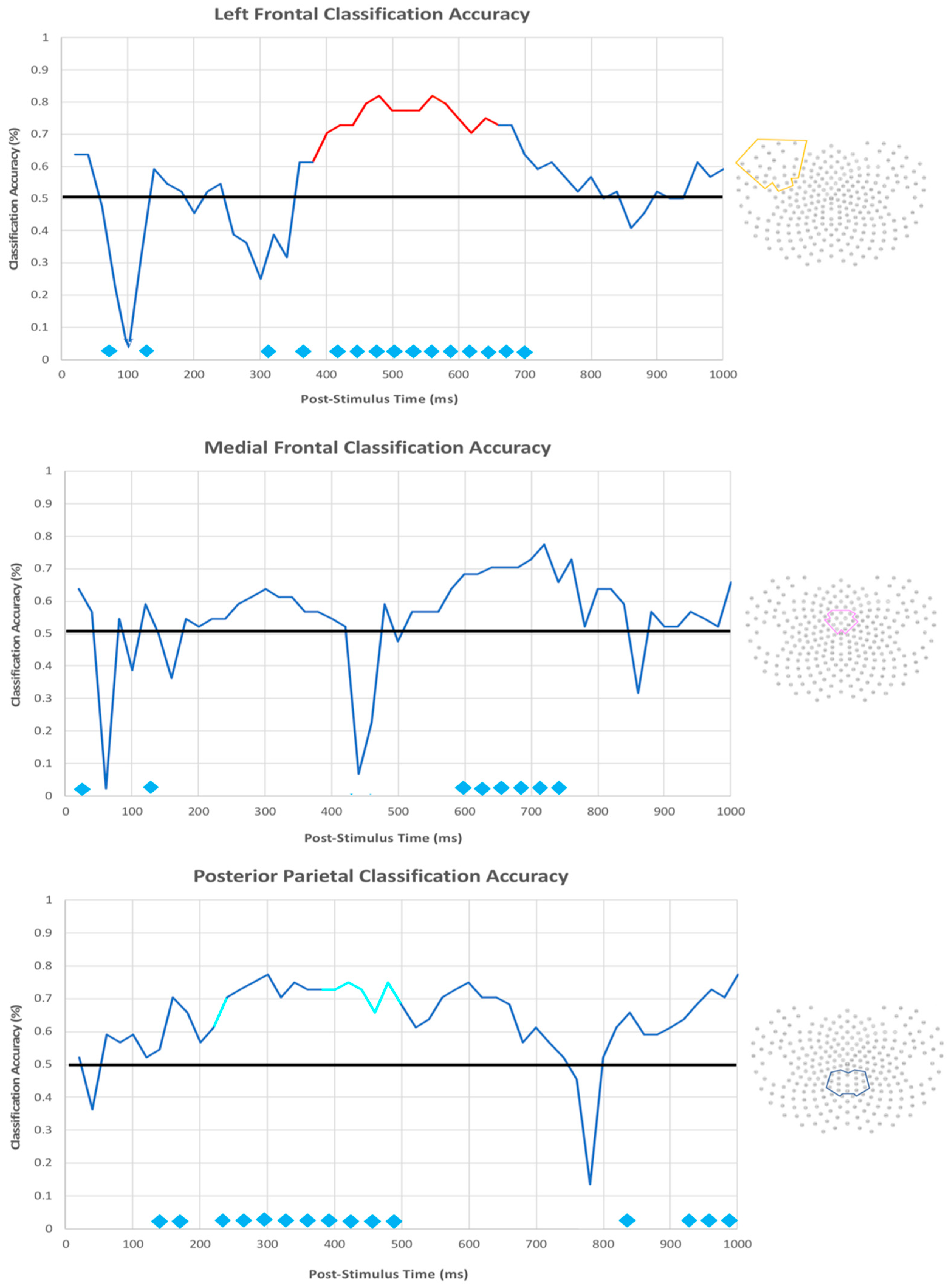
3.2.3. EEG Machine Learning Analysis
4. Discussion
4.1. fMRI Pilot Experiment
4.1.1. Univariate Analysis
4.1.2. Multi-Voxel Pattern Analysis
4.2. Experiment 2 (dEEG)
4.2.1. ERPs
4.2.2. dEEG Machine Learning
4.3. Category Learning Strategies as a Function of Expertise
4.4. Alternative Interpretations and Limitations
5. Conclusions
Author Contributions
Funding
Conflicts of Interest
References
- Bruner, J.; Goodnow, J.J.; Austin, G.A. A Study of Thinking; Science Editions: New York, NY, USA, 1967. [Google Scholar]
- Schneider, W.; Shiffrin, R.M. Controlled and automatic human information processing: I. Detection, search, and attention. Psychol. Rev. 1977, 84, 1–66. [Google Scholar] [CrossRef]
- Zeithamova, D.; Maddox, W.T. Dual task interference in perceptual category learning. Mem. Cogn. 2006, 34, 387–398. [Google Scholar] [CrossRef] [PubMed] [Green Version]
- Knowlton, B.J.; Squire, L.R. The learning of categories: Parallel brain systems for item memory and category knowledge. Science 1993, 262, 1747–1749. [Google Scholar] [CrossRef] [PubMed] [Green Version]
- Gabrieli, J.D.E. Cognitive neuroscience of human memory. Annu. Rev. Psychol. 1998, 49, 87–115. [Google Scholar] [CrossRef] [Green Version]
- Smith, E.E.; Patalano, A.L.; Jonides, J. Alternative strategies of categorization. Cognition 1998, 65, 167–196. [Google Scholar] [CrossRef] [Green Version]
- Casale, M.B.; Ashby, F.G. A role for the perceptual representation memory system in category learning. Percept. Psychophys. 2008, 70, 983–999. [Google Scholar] [CrossRef] [Green Version]
- Chein, J.M.; Schneider, W. Neuroimaging studies of practice-related change: fMRI and meta-analytic evidence of a domain-general control network for learning. Cogn. Brain Res. 2005, 25, 607–623. [Google Scholar] [CrossRef]
- Gabriel, M.; Burhans, L.; Talk, A.; Scalf, P. Cingulate cortex. In Encyclopedia of the Human Brain; Ramachandran, V.S., Ed.; Elsevier Science: Amsterdam, The Netherlands, 2002; pp. 775–791. [Google Scholar]
- Schneider, G.E. Two visual systems. Science 1969, 163, 895–902. [Google Scholar] [CrossRef]
- Ungerleider, L.G.; Mishkin, M. Two cortical visual systems. In Analysis of Visual Behavior; Ingle, D.J., Goodale, M.A., Mansfield, R.J.W., Eds.; MIT Press: Cambridge, MA, USA, 1982; pp. 549–586. [Google Scholar]
- Keele, S.W.; Ivry, R.; Mayr, U.; Hazeltine, E.; Heuer, H. The cognitive and neural architecture of sequence representation. Psychol. Rev. 2003, 110, 316–339. [Google Scholar] [CrossRef] [Green Version]
- Luu, P.; Jiang, Z.; Poulsen, C.; Mattson, C.; Smith, A.; Tucker, D.M. Learning and the development of contexts for action. Front. Hum. Neurosci. 2011, 5, 159. [Google Scholar] [CrossRef] [Green Version]
- Kemler-Nelson, D.G. The effect of intention on what concepts are acquired. J. Verbal Learn. Verbal Behav. 1984, 23, 734–759. [Google Scholar] [CrossRef]
- Ashby, F.G.; Alfonso-Reese, L.A.; Turken, A.U.; Waldron, E.M. A neuropsychological theory of multiple systems in category learning. Psychol. Rev. 1998, 105, 442–481. [Google Scholar] [CrossRef] [PubMed] [Green Version]
- Rosch, E. Cognitive representations of semantic categories. J. Exp. Psychol. Gen. 1975, 104, 192–233. [Google Scholar] [CrossRef]
- Rosch, E. Principles of Categorization; Lawrence Erlbaum Associates: Hillsdale, NJ, USA, 1978. [Google Scholar]
- Aizenstein, H.J.; MacDonald, A.W.; Stenger, V.A.; Nebes, R.D.; Larson, J.K.; Ursu, S.; Carter, C.S. Complementary category learning systems identified using event-related functional mri. J. Cogn. Neurosci. 2000, 12, 977–987. [Google Scholar] [CrossRef] [PubMed]
- Reber, P.J.; Stark, C.E.L.; Squire, L.R. Contrasting cortical activity associated with category memory and recognition memory. Learn. Mem. 1998, 5, 420–428. [Google Scholar] [PubMed]
- Reber, P.J.; Squire, L.R. Intact learning of artificial grammars and intact category learning by patients with Parkinson’s disease. Behav. Neurosci. 1999, 113, 235–242. [Google Scholar] [CrossRef] [PubMed]
- Nosofsky, R.M. Attention, similarity, and the identification-categorization relationship. J. Exp. Psychol. Gen. 1986, 115, 39–57. [Google Scholar] [CrossRef]
- Ashby, F.G.; Ell, S.W. The neurobiology of human category learning. Trends Cogn. Sci. 2001, 5, 204–210. [Google Scholar] [CrossRef]
- Waldron, E.M.; Ashby, F.G. The effects of concurrent task interference on category learning: Evidence from multiple category learning systems. Psychon. Bull. Rev. 2001, 8, 168–176. [Google Scholar] [CrossRef]
- Minda, J.P.; Miles, S.J. The influence of verbal and nonverbal processing on category learning. Psychol. Learn. Motiv. 2010, 52, 117–162. [Google Scholar]
- Dale, A.M. Optimal experimental design for event-related mri. Hum. Brain Mapp. 1999, 8, 109–114. [Google Scholar] [CrossRef]
- Jenkinson, M.; Beckmann, C.F.; Behrens, T.E.; Woolrich, M.W.; Smith, S.M. FSL. NeuroImage 2012, 62, 782–790. [Google Scholar] [CrossRef] [PubMed] [Green Version]
- Worsley, K.J. Statistical analysis of activation images. In Functional Mri: An Introduction to Methods; Jezzard, P., Matthews, P.M., Smith, S.M., Eds.; Oxford University Press: New York, NY, USA, 2001; pp. 251–270. [Google Scholar]
- Nomura, E.M.; Maddox, W.T.; Filoteo, J.V.; Ing, A.D.; Gitelman, D.R.; Parrish, T.B.; Mesulam, M.M.; Reber, P.J. Neural correlates of rule-based and information-integration visual category learning. Cereb. Cortex 2006, 17, 37–43. [Google Scholar] [CrossRef] [PubMed] [Green Version]
- Norman, K.A.; Polyn, S.M.; Deltre, G.J.; Haxby, J.V. Beyond mind-reading: Multi-voxel pattern analysis of fMRI data. Trends Cogn. Sci. 2006, 10, 424–430. [Google Scholar] [CrossRef]
- Dale, A.M.; Fischl, B.; Sereno, M.I. Cortical surface-based analysis. I. Segmentation and surface reconstruction. NeuroImage 1999, 9, 179–194. [Google Scholar] [CrossRef]
- Fischl, B.; Salat, D.H.; Busa, E.; Albert, M.; Dieterich, M.; Haselgrove, C.; van der Kouwe, A.; Killiany, R.; Kennedy, D.; Klaveness, S.; et al. Whole brain segmentation: Automated labeling of neuroanatomical structures in the human brain. Neuron 2002, 33, 341–355. [Google Scholar] [CrossRef] [Green Version]
- Woolgar, A.; Thompson, R.; Bor, D.; Duncan, J. Multi-voxel coding of stimuli, rules, and responses in human frontoparietal cortex. NeuroImage 2011, 56, 744–752. [Google Scholar] [CrossRef]
- Reverberi, C.; Görgen, K.; Haynes, J.D. Compositionality of rule representations in human prefrontal cortex. Cereb. Cortex 2012, 22, 1237–1246. [Google Scholar] [CrossRef] [Green Version]
- Nelissen, N.; Strokes, M.; Nobre, A.C.; Rushworth, M.F. Frontal and parietal cortical interactions with distributed visual representations during selection attention and action selection. J. Neurosci. 2013, 33, 16443–16458. [Google Scholar] [CrossRef] [Green Version]
- Rissman, J.; Gazzaley, A.; D’Esposito, M. Measuring functional connectivity during distinct stages of a cognitive task. NeuroImage 2004, 23, 752–763. [Google Scholar] [CrossRef]
- Avants, B.B.; Tustison, N.J.; Song, G.; Cook, P.A.; Klein, A.; Gee, J.C. A reproducible evaluation of ANTs similarity metric performance in brain image registration. NeuroImage 2011, 54, 2033–2044. [Google Scholar] [CrossRef] [PubMed] [Green Version]
- Mur, M.; Bandettini, P.A.; Kriegeskorte, N. Revealing representational content with pattern-information fMRI—An introductory guide. Soc. Cogn. Affect. Neurosci. 2009, 4, 101–109. [Google Scholar] [CrossRef] [PubMed]
- Esterman, M.; Tamber-Rosenau, B.J.; Chiu, Y.; Yantis, S. Avoiding non-independence in fMRI data analysis: Leave one subject out. NeuroImage 2010, 50, 572–576. [Google Scholar] [CrossRef] [PubMed] [Green Version]
- Luu, P.; Tucker, D.M.; Stripling, R. Neural mechanisms for learning action in context. Brain Res. 2007, 1179, 89–105. [Google Scholar] [CrossRef]
- Morgan, K.K.; Luu, P.; Tucker, D.M. Changes in p3b latency and amplitude reflect expertise acquisition in a football visuomotor learning task. PLoS ONE 2016, 11, e0154021. [Google Scholar] [CrossRef] [PubMed] [Green Version]
- Bush, G.; Vogt, B.A.; Holmes, J.; Dale, A.M.; Greve, D.; Jenike, M.A.; Rosen, B.R. Dorsal anterior cingulate cortex: A role in reward-based decision making. Proc. Natl. Acad. Sci. USA 2002, 99, 523–528. [Google Scholar] [CrossRef] [PubMed] [Green Version]
- Halgren, E.; Baudena, P.; Heit, G.; Clarke, J.M.; Marinkovic, K.; Chauvel, P. Spatio-temporal stages in face and word processing. 2. Depth-recorded potentials in the human frontal and Rolandic cortices. J. Physiol. 1994, 88, 51–80. [Google Scholar] [CrossRef]
- Halgren, E.; Baudena, P.; Clarke, J.M.; Heit, G.; Liegeois, C.; Chauvel, P.; Musolino, A. Intracerebral potential to rare target and distractor auditory and visual stimuli. I. Superior temporal plane and parietal lobe. Electroencephalogr. Clin. Neurophysiol. 1995, 94, 191–220. [Google Scholar] [CrossRef]
- Halgren, E.; Baudena, P.; Clarke, J.M.; Heit, G.; Marinkovic, K.; Devaux, B.; Vignal, J.P.; Biraben, A. Intracerebral potential to rare target and distractor auditory and visual stimuli. II. Medial, lateral, and posterior temporal lobe. Electroencephalogr. Clin. Neurophysiol. 1995, 94, 229–250. [Google Scholar] [CrossRef]
- Baudena, P.; Halgren, E.; Heit, G.; Clarke, J.M. Intracerebral potentials to rare target and distractor auditory and visual stimuli. III. Frontal cortex. Electroencephalogr. Clin. Neurophysiol. 1995, 94, 251–264. [Google Scholar] [CrossRef]
- Smith, M.E.; Halgren, E.; Sokolik, M.; Baudena, P.; Musolino, A.; Liegeois-Chauvel, C.; Chauvel, P. The intracranial topography of the p3 event-related potential elicited during auditory oddball. Electroencephalogr. Clin. Neurophysiol. 1990, 76, 235–248. [Google Scholar] [CrossRef]
- Brankack, J.; Seidenbecher, T.; Muller-Gartner, H.W. Task-relevant late positive component in rats: Is it related to hippocampal theta rhythm? Hippocampus 1996, 6, 475–482. [Google Scholar] [CrossRef]
- Shin, J. The interrelationship between movement and cognition: Theta rhythm and the p330 event-related potential. Hippocampus 2011, 21, 744–752. [Google Scholar] [CrossRef] [PubMed]
- Kahana, M.J.; Seelig, D.; Madsen, J.R. Theta returns. Curr. Opin. Neurobiol. 2001, 11, 739–744. [Google Scholar] [CrossRef]
- Miles, S.J.; Matsuki, K.; Minda, J.P. Continuous executive function disruption interferes with application of an information integration categorization strategy. Atten. Percept. Psychophys. 2014, 76, 1318–1334. [Google Scholar] [CrossRef]
- Lombardi, W.J.; Andreason, P.J.; Sirocco, K.Y.; Rio, D.E.; Gross, R.E.; Umhau, J.C.; Hommer, D.W. Wisconsin card sorting test performance following head-injury: Dorsolateral fronto-striatal circuit activity predicts perseveration. J. Exp. Neuropsychol. 1999, 21, 2–16. [Google Scholar] [CrossRef]
- Rao, S.M.; Bobholz, J.A.; Hammeke, T.A.; Tosen, A.C.; Woodley, S.J.; Cunningham, J.M.; Cox, R.W.; Stein, E.A.; Binder, J.R. Functional mri evidence for subcortical participation in conceptual reasoning skills. Neuroreport 1997, 8, 1987–1993. [Google Scholar] [CrossRef]
- Rogers, R.D.; Andrews, T.C.; Grasby, P.M.; Brooks, D.J.; Robbins, T.W. Contrasting cortical and subcortical activations produced by attentional-set shifting and reversal learning in humans. J. Cogn. Neurosci. 2000, 12, 142–162. [Google Scholar] [CrossRef]
- Ashby, F.G.; Paul, E.J.; Maddox, W.T. COVIS. In Formal Approaches in Categorization; Pothos, E.M., Wills, A.J., Eds.; Cambridge University Press: New York, NY, USA, 2011; pp. 65–87. [Google Scholar]
- Eichenbaum, H. A cortical-hippocampal system for declarative memory. Nat. Rev. Neurosci. 2000, 1, 41–50. [Google Scholar] [CrossRef]
- Haynes, J.D.; Rees, G. Decoding mental states from brain activity in humans. Nat. Rev. Neurosci. 2006, 7, 523–534. [Google Scholar] [CrossRef]
- Desimone, R.; Duncan, J. Neural mechanisms of selective visual attention. Annu. Rev. Neurosci. 1995, 18, 193–222. [Google Scholar] [CrossRef] [PubMed]
- Miller, E.K.; Cohen, J.D. An integrative theory of prefrontal cortex function. Annu. Rev. Neurosci. 2001, 24, 167–202. [Google Scholar] [CrossRef] [PubMed]
- Asaad, W.F.; Rainer, G.; Miller, E.K. Neural activity in the primate prefrontal cortex during associative learning. Neuron 1998, 21, 1399–1407. [Google Scholar] [CrossRef] [Green Version]
- Freedman, D.J.; Assad, J.A. Experience-dependent representation of visual categories in parietal cortex. Nature 2006, 443, 85–88. [Google Scholar] [CrossRef] [PubMed]
- White, I.M.; Wise, S.P. Rule-dependent neuronal activity in the prefrontal cortex. Exp. Brain Res. 1999, 126, 315–335. [Google Scholar] [CrossRef] [PubMed]
- Bode, S.; Haynes, J.D. Decoding sequential stages of task preparation in the human brain. NeuroImage 2009, 45, 606–613. [Google Scholar] [CrossRef] [PubMed]
- Haynes, J.D.; Sakai, K.; Rees, G.; Gilbert, S.; Frith, C.; Passingham, R.E. Reading hidden intentions in the human brain. Curr. Biol. 2007, 17, 323–328. [Google Scholar] [CrossRef] [Green Version]
- Toni, I.; Rammani, N.; Josephs, O.; Ashburner, J.; Passingham, R.E. Learning arbitrary visuomotor associations: Temporal dynamics of brain activity. NeuroImage 2001, 14, 1048–1057. [Google Scholar] [CrossRef]
- Groll, M.J.; de Lange, F.P.; Verstraten, F.A.J.; Passingham, R.E.; Toni, I. Cerebral changes during performance of overlearned arbitrary visuomotor associations. J. Neurosci. 2006, 26, 117–125. [Google Scholar] [CrossRef]
- Donchin, E.; Coles, M.G.H. Is the p300 component a manifestation of context updating? Behav. Brain Sci. 1988, 11, 357–374. [Google Scholar] [CrossRef]
- Palmeri, T.J. Exemplar similarity and the development of automaticity. J. Exp. Psychol. Learn. Mem. Cogn. 1997, 23, 324–354. [Google Scholar] [CrossRef] [PubMed]
- Nosofsky, R.M.; Palmeri, T.J.; McKinley, S.C. Rule-plus-exception model of classification learning. Psychol. Rev. 1994, 101, 53–79. [Google Scholar] [CrossRef] [PubMed]
- Palmeri, T.J.; Nosofsky, R.M. Recognition memory for exceptions to the category rule. J. Exp. Psychol. Learn. Mem. Cogn. 1995, 21, 548–568. [Google Scholar] [CrossRef] [PubMed]
- Zeithamova, D.; Maddox, W.T.; Schnyer, D.M. Dissociable prototype learning systems: Evidence from brain imaging and behavior. J. Neurosci. 2008, 28, 13194–13201. [Google Scholar] [CrossRef] [PubMed]


| Location | Cluster Size | Z-Value | X | Y | Z |
|---|---|---|---|---|---|
| L Sup. Fr. Gyrus | 58 | 2.79 | −54 | 44 | −10 |
| L. IFG | 50 | 2.95 | −50 | 30 | 14 |
| L. Sup. Fr. Gyrus | 38 | 2.72 | −12 | 40 | 56 |
| L. Sup. Fr. Gyrus | 34 | 2.47 | −16 | 56 | 38 |
| R. Hippocampus | 26 | 2.88 | 22 | −34 | −10 |
| L. Sup. Temp. Gyrus | 25 | 2.67 | −50 | 10 | −16 |
| R. Fusiform Gyrus | 25 | 3.04 | 40 | −44 | −20 |
| R. Lateral Occipital Cortex | 24 | 2.72 | −10 | −12 | 56 |
| L. Suppl. Motor Cortex | 22 | 2.42 | 58 | −64 | 24 |
| Brain Stem | 22 | 2.63 | 6 | −22 | −28 |
| R. Mid. Temp. Gyrus | 20 | 2.56 | 40 | −58 | 2 |
| Location | Cluster Size | Z-Value | X | Y | Z |
|---|---|---|---|---|---|
| R. Lateral Occipital Cortex | 519 | 3.16 | 6 | −74 | 36 |
| R. Lateral Occipital Cortex | 154 | 2.87 | 34 | −62 | 62 |
| L. Fusiform Gyrus | 106 | 3.17 | −20 | −66 | −18 |
| L. Lateral Occipital Cortex | 98 | 2.83 | −36 | −56 | 38 |
| R. IFG | 89 | 3.25 | 20 | 56 | −6 |
| L. Post. Cingulate Gyrus | 70 | 2.88 | −8 | −40 | 48 |
| R. Lateral Occipital Cortex | 55 | 2.47 | 20 | −88 | 38 |
| R. Fusiform Gyrus | 52 | 2.62 | 20 | −54 | −16 |
| L. Middle Frontal Gyrus | 49 | 2.77 | −38 | 45 | 18 |
| R. Occipital Pole | 41 | 2.34 | 20 | −104 | −10 |
| Brain Stem | 40 | 3.05 | 22 | −32 | −42 |
| Location | Cluster Size | Z-Value | X | Y | Z |
|---|---|---|---|---|---|
| L. Caudate Nucleus | 290 | 3.5 | −8 | −10 | 24 |
| Cerebellum | 129 | 3.22 | 16 | −72 | −28 |
| Cerebellum | 125 | 3.43 | 32 | −80 | −22 |
| Cerebellum | 90 | 3.18 | 4 | −50 | −10 |
| L. Sup. Frontal Gyrus | 88 | 3.21 | −28 | 6 | 64 |
| L. Lateral Occipital Cortex | 73 | 3.17 | −26 | −78 | 50 |
| R. Lateral Occipital Cortex | 71 | 3.08 | 40 | −74 | 42 |
| L. Inf. Frontal Gyrus | 67 | 3.22 | −42 | 22 | 4 |
| Cerebellum | 63 | 3.3 | −26 | −90 | −26 |
| L. Sup. Frontal Gyrus | 59 | 3.17 | −42 | 46 | 20 |
| Brain Stem | 58 | 2.92 | 14 | −16 | −38 |
| Location | Cluster Size | Z-Value | X | Y | Z |
|---|---|---|---|---|---|
| R. Lateral Occipital Cortex | 1922 | 4 | 18 | −100 | 6 |
| R. Fusiform Gyrus | 335 | 3.41 | 12 | −72 | −2 |
| R. Inf. Frontal Gyrus | 213 | 3.11 | 62 | 6 | 12 |
| Postcentral Gyrus | 144 | 3.35 | −40 | −26 | 54 |
| L. Sup. Temporal Gyrus | 143 | 3.49 | 68 | −24 | 28 |
| Cerebellum | 113 | 3.09 | −20 | −72 | −52 |
| L. Fusiform Gyrus | 100 | 2.88 | 38 | −54 | −24 |
| R. Mid. Temporal Gyrus | 99 | 3.13 | 66 | −40 | 2 |
| R. Mid. Frontal Gyrus | 82 | 3.25 | 32 | 18 | 30 |
| R. Mid Temporal Gyrus | 79 | 3.37 | 54 | −6 | −28 |
| R. Angular Gyrus | 70 | 3.7 | 56 | −46 | 30 |
© 2020 by the authors. Licensee MDPI, Basel, Switzerland. This article is an open access article distributed under the terms and conditions of the Creative Commons Attribution (CC BY) license (http://creativecommons.org/licenses/by/4.0/).
Share and Cite
K. Morgan, K.; Zeithamova, D.; Luu, P.; Tucker, D. Spatiotemporal Dynamics of Multiple Memory Systems During Category Learning. Brain Sci. 2020, 10, 224. https://doi.org/10.3390/brainsci10040224
K. Morgan K, Zeithamova D, Luu P, Tucker D. Spatiotemporal Dynamics of Multiple Memory Systems During Category Learning. Brain Sciences. 2020; 10(4):224. https://doi.org/10.3390/brainsci10040224
Chicago/Turabian StyleK. Morgan, Kyle, Dagmar Zeithamova, Phan Luu, and Don Tucker. 2020. "Spatiotemporal Dynamics of Multiple Memory Systems During Category Learning" Brain Sciences 10, no. 4: 224. https://doi.org/10.3390/brainsci10040224