Methane Detection Based on Improved Chicken Algorithm Optimization Support Vector Machine

Abstract

Methane, known as a flammable and explosion hazard gas, is the main component of marsh gas, firedamp, and rock gas. Therefore, it is important to be able to detect methane concentration safely and effectively. At present, many models have been proposed to enhance the performance of methane predictions. However, the traditional models displayed inevitable shortcomings in parameter optimization in our experiment, which resulted in their having poor prediction performance. Accordingly, the improved chicken swarm algorithm optimized support vector machine (ICSO-SVM) was proposed to predict the concentration of methane precisely. The traditional chicken swarm optimization algorithm (CSO) easily falls into a local optimum due to its characteristics, so the ICSO algorithm was developed. The formula for position updating of the chicks of the ICSO is not only about the rooster of the same subgroup, but also about the roosters of other subgroups. Therefore, the ICSO algorithm more easily avoids falling into the local extremum. In this paper, the following work has been done. The sample data were obtained by using the methane detection system designed by us; In order to verify the validity of the ICSO algorithm, the ICSO, CSO, genetic algorithm (GA), and particle swarm optimization algorithm (PSO) algorithms were tested, and the four models were applied for methane concentration prediction. The results showed that he ICSO algorithm had the best convergence effect, relative error percentage, and average mean squared error, when the four models were applied to predict methane concentration. The results showed that the average mean squared error values of ICSO-SVM model were smaller than other three models, and that the ICSO-SVM model has better stability, and the average recovery rate of the ICSO-SVM is much closer to 100%. Therefore, the ICSO-SVM model can efficiently predict methane concentration.

1. Introduction

Air pollution is a serious environmental issue that has attracted more and more attention globally in recent years [1,2,3]. Methane is the main greenhouse pollutant, and also the main component of mine gas, biogas, and various liquid fuels [4,5]. It is stipulated that the lowest limit of explosion in air is 5.0%, the highest limit is 15.0%, and the explosive capacity is the strongest when the volume fraction is 9.5% [6]. Methane in the atmosphere can also cause a greenhouse effect and accelerate global warming [7,8]. It is for these reasons that methane detection is an indispensable field of research. Traditional detection generally adopts chemical methods, which require chemical reagents. These reagents have many disadvantages, such as danger, need to replace, and short life, and so these methods are not conducive to online real-time detection. In addition, absorption spectroscopy is a detection method that offers a rapid, direct, and selective technique to measure the concentration of methane [9], and it has become the dominant detecting method [10,11]. Methane concentrations are obtained through infrared spectroscopy with an appropriate forecasting model.

Currently, it is urgent that an accurate and effective methane prediction model be developed, such as least squares fit, multi-element linear regression, back propagation neural network, or support vector machine (SVM). SVM, based on the principle of structural risk minimization, has higher efficiency when the number of training samples is small [12,13]. The performance of SVM is highly related to its kernel parameters and penalty factor, so choosing appropriate parameters is the key to improving the prediction accuracy. At present, there are a lot of parameter optimization algorithms. For example, Zhou and Lu used the genetic algorithm (GA) to select features and optimize the SVM parameters to improve the prediction accuracy of a hospitalization expense model [14]. Wang and Guan used the particle swarm optimization algorithm optimized support vector machine (PSO-SVM) classifier to classify the maximum tensile shear strength of spot-welded joints; the results showed that the PSO-SVM classifier had a good accuracy [15]. The PSO-SVM based on adaptive mutation was used to classify the increased volume and complexity of flow cytometry (FCM) data by Wang [16]. Liu proposed a short-term wind speed forecasting method, which consists of ensemble empirical mode decomposition (EEMD) for data preprocessing, and an SVM optimized by the cuckoo search algorithm (CS). The experimental results indicated that the proposed model can not only improve the forecasting accuracy, but also can be an effective tool in assisting the management of wind power plants [17]. A new cuckoo search algorithm based on a chaotic catfish effect optimization of the SVM was proposed by He and Xia, who applied it to oil layer recognition [18]. Dai and Niu proposed a SVM optimization based on differential evolution and the grey wolf optimization (DE-GWO-SVM) algorithm to predict power grid investment, which proved that the DE-GWO-SVM model had strong generalization capacity and had a good prediction effect on power grid investment forecasting in China [19].

The CSO algorithm, known as a novel nature-inspired algorithm, was proposed by Meng Xianbing in 2014 [20]. CSO is a stochastic optimization method based on the search behavior of the chicken, which simulates the hierarchy order and the behaviors of a chicken swarm. The chicken swarm is divided into subgroups, and each subgroup consists of chicks, some hens, and a rooster. There is competition between subgroups, that is to say, there is a global optimization result. However, in the paper [18], it was indicated that CSO easily falls into a local optimum, and its progress and speed are greatly influenced by initial values. To this end, an ICSO is proposed. In the ICSO algorithm, a position update equation was added the chicks’ learning from the rooster, and learning factors of the chicks were introduced. The convergence accuracy of ICSO is improved, and the ICSO algorithm can easily jump out of the local optimal [21]. The ICSO algorithm has been applied variously in many fields. In Reference [22], the ICSO algorithm was applied in tracking control of the maximum power point of a photovoltaic system. Liang and Wang employed an ICSO algorithm to improve the efficiency of synthetic aperture radar (SAR) image segmentation [23] and so on. However, no paper has yet reported on the application of ICSO algorithm in gas detection.

Based on the above research, this paper proposes a prediction model for methane based on ICSO and SVM. The methane concentration is predicted by SVM, and the ICSO is used to optimize the penalty factor and kernel parameters of SVM. To validate the performance of ICSO-SVM model, the parameters of SVM were also optimized by CSO, GA, and PSO. This paper is organized as follows: Section 2 introduces the methodology, including the SVM, CSO, and ICSO algorithms, and proposes the ICSO-SVM forecasting model. Section 3 gives a brief introduction to the evaluation criteria for forecasting performance. The experiment device and its performance analysis are introduced in Section 4. In Section 5, the results and the superiority of the ICSO-optimized SVM are discussed, using comparisons with the CSO-, GA-, and PSO-optimized SVM. Finally, Section 6 summarizes this paper.

2. Methodology

2.1. SVM

The SVM was proposed by Vapnik in 1995 [24,25]. SVM, as a machine learning method, is effective for small samples, nonlinear, high dimensional, etc. SVM is developed from solving linear problems; it can construct an optimal hyperplane under the condition of linear and divisible. However, in practical applications, most problems are nonlinear. Therefore, the nonlinear input data map to a high-dimensional feature space. For example, given a set of array lengths n, which belong to R^d:

$$\begin{gathered} ({\mathit{x}}_1,y_1),({\mathit{x}}_2,y_2),\dots ,({\mathit{x}}_n,y_n) \\ {\mathit{x}}_i\in {\mathbf{R}}^d,y_i\in \{-1,+1\},i=1,\dots ,n \end{gathered}$$

(1)

where x_i ∈ R^d are input training samples, y_i are training samples, and d is dimension.

If the samples are separable, there is a classification hyperplane that separates the two types of samples. Crosses and open circles represent two types of samples in Figure 1, respectively. The nearest points to the classified hyperplane are named the support vector. H is a classification hyperplane. Hyperplanes H₁ and H₂ are linked to two types of support vectors and are parallel to H. The distance between H₁ and H is equal to the distance between H₂ and H. The distance between H₁ and H₂ is called the classification interval.

A hyperplane divides the data into two categories, as follows:

$$\{\begin{array}{c}(\mathit{w}·{\mathit{x}}_i)+\mathrm{b}\ge 0,y_i=+1\\ (\mathit{w}·{\mathit{x}}_i)+\mathrm{b}\le 0,y_i=-1\end{array}$$

(2)

where w is the vector of the hyperplane, x is the input vector of the training set, and b is the constant term of the hyperplane. A hyperplane over two types of sample support vector is defined as:

$$\{\begin{array}{c}(\mathit{w}·{\mathit{x}}_i)+\mathrm{b}=+1\\ (\mathit{w}·{\mathit{x}}_i)+\mathrm{b}=-1\end{array}$$

(3)

The interval d between hyperplanes H₁ and H₂ can be obtained from Equation (3):

$$d=\frac{2}{\left|\mathit{w}\right|}$$

(4)

The regression function of classification of the hyperplane is defined as:

$$f(\mathit{x})=(\mathit{w}·\mathit{x})+\mathrm{b},\mathit{w}\in {\mathbf{R}}^d,\mathrm{b}\in \mathbf{R}$$

(5)

The optimal hyperplane has a maximum margin between two classes. The optimal hyperplane problem is transformed into solving the quadratic optimization, and the slack variable is introduced [26]. The quadratic form can be represented as:

$$\begin{array}{c}\min \frac{1}{2}{\Vert \mathit{w}\Vert }^2+C{\displaystyle \sum _{i=1}^n{\xi }_i}+{\xi }_i^{*}\\ s.t.\{\begin{array}{c}{y}_i-(\mathit{w}·{\mathit{x}}_i)-\mathrm{b}\le \epsilon +{\xi }_i\\ (\mathit{w}·{\mathit{x}}_i)+\mathrm{b}-y_i\le \epsilon +{\xi }_i^{*}\\ {\xi }_i,{\xi }_i^{*}\ge 0\end{array}\end{array}\}$$

(6)

where ${\xi }_i,{\xi }_i^{*}$ are relaxation factors, C is the penalty factor, ε is the insensitivity coefficient, and s.t. is constraint.

Due to the complexity of the calculations of the quadratic optimization, the Equation (6) is transformed into a dual problem with Lagrange duality theory, as Equation (7) and (8)

$$\begin{array}{ll}\mathrm{L}(\mathit{w},{\xi }_i,{\xi }_i^{*},\alpha ,{\alpha }^{*},\mathrm{C},\beta ,{\beta }^{*})& =\frac{1}{2}{\Vert \mathit{w}\Vert }^2+\mathrm{C}{\displaystyle \sum _{i=1}^n{\xi }_i}+{\xi }_i^{*}\\ & -{\displaystyle \sum _{i=1}^n{\alpha }_i[(\mathit{w}·{\mathit{x}}_i)+\mathrm{b}-y_i+\epsilon +{\xi }_i]}\\ & -{\displaystyle \sum _{i=1}^n{\alpha }_i^{*}[y_i-(\mathit{w}·{\mathit{x}}_i)-\mathrm{b}+\epsilon +{\xi }_i^{*}]}\\ & -{\displaystyle \sum _{i=1}^n({\beta }_i{\xi }_i+{\beta }_i^{*}{\xi }_i^{*})}\end{array}$$

(7)

where α_i, α_i*, β_i, β_i* are all Lagrange multipliers.

$$\begin{array}{c}\begin{array}{l}\underset{{\alpha }_i,{\alpha }_i^{*}}{\max }-\epsilon {\displaystyle \sum _{i=1}^l(}{\alpha }_i+{\alpha }_i^{*})+{\displaystyle \sum _{i=1}^l{y}_i}({\alpha }_i-{\alpha }_i^{*})\\ -\frac{1}{2}{\displaystyle \sum _{i,j=1}^l(}{\alpha }_i-{\alpha }_i^{*})({\alpha }_j-{\alpha }_j^{*})({\mathit{x}}_i·{\mathit{x}}_j)\end{array}\\ s.t.\{\begin{array}{c}{\displaystyle \sum _{i=1}^l(}{\alpha }_i-{\alpha }_i^{*})=0\\ {\alpha }_i,{\alpha }_i^{*}\in [0,\mathrm{C}]\end{array}\end{array}\}$$

(8)

The expression of f(x) in Equation (5) is expressed as:

$$f(\mathit{x})={\displaystyle \sum _{i=1}^l{\beta }_i}({\mathit{x}}_i·\mathit{x})+\mathrm{b}$$

(9)

β_i is non-support vector. When the data set is certain, β_i = 0. The f(x) is represented by the remaining support vectors as:

$$f(\mathit{x})={\displaystyle \sum _{i\in \mathrm{N}}{\beta }_i({\mathit{x}}_i·\mathit{x})+\mathrm{b}}$$

(10)

where N is a subset of the input data set. For a particular problem, a model for this problem can be determined by a subset of given data. When the problem is nonlinear, Equation (10) cannot accurately represent f(x). The nonlinear input data map to a high-dimensional feature space using nonlinear mapping Φ(x). In order to reduce the amount of calculation involved, the inner product operation of the high-dimensional feature space is converted into a function transport of the input space by using the kernel function K(x_i, x).

$$K({\mathit{x}}_i,{\mathit{x}}_j)=(\Phi ({\mathit{x}}_i)·\Phi ({\mathit{x}}_j))$$

(11)

The expression of f(x) of Equation (10) can be expressed as:

$$f(\mathit{x})={\displaystyle \sum _{i\in \mathrm{N}}{\beta }_i}K({\mathit{x}}_i,\mathit{x})+\mathrm{b}$$

(12)

Common kernel functions include the linear kernel function, polynomial kernel function, sigmoid kernel function, and Gaussian radical kernel function. The Gaussian radical kernel function is better for problems with less a priori information [20]. The expression of the Gaussian radical kernel function is expressed as:

$$K({\mathit{x}}_i,{\mathit{x}}_j)=\exp \left(-\frac{{\Vert {\mathit{x}}_i-{\mathit{x}}_j\Vert }^2}{2r^2}\right)$$

(13)

where r is the radius of radial basis kernel function, and g = 2r² is the kernel parameter.

The values of g and penalty factor C heavily affect the performance of SVM. The ICSO algorithm is intended to optimize the parameters of SVM rather than relying on random selection.

2.2. Chicken Swarm Optimization Algorithm (CSO)

The CSO algorithm is a kind of bionic random search algorithm, which imitates the foraging behaviors of a chicken swarm. The CSO algorithm consists of several subgroups. Each subgroup consists of a rooster, some hens, and several chicks. The roosters have the best fitness value, and the chicks have the worst fitness value. The position of each individual (roosters, hens, and chicks) represents a solution of the problem. The rooster has the best search ability compared to hens and chicks in each subgroup.

The rooster is a leader of the subgroup, with its position update equation defined by the following:

$${\mathit{x}}_{i,j}\left(t+1\right)={\mathit{x}}_{i,j}\left(t\right)\cdot \left(1+\Phi \left(0,{\sigma }^2\right)\right)$$

(14)

$${\sigma }^2=\{\begin{array}{c}1,f_{ir}\le f_{kr}\\ \exp \left(\frac{f_{kr}-f_{ir}}{\left|f_{ir}\right|+\epsilon }\right)\end{array}$$

(15)

where x_i,j(t + 1) is the position of the rooster at the time t + 1. x_i,j(t) is the position of at the time t. i is the subgroup number, j is the rooster index, Φ(0, σ²) is the Gaussian distribution with zero mean and standard deviation σ. f_ir and f_kr are the fitness value of rooster, which is randomly selected (k ≠ i). ε is the smallest constant that is not equal to 0.

The hens follow the rooster when foraging, so their position is affected by roosters in both the same subgroup and other subgroups. Hens’ position update equation is as follows:

$$x_{i,j}\left(t+1\right)=x_{i,j}\left(t\right)+C_1\cdot rand\cdot \left(x_{r_1,j}\left(t\right)-x_{i,j}\left(t\right)\right)+C_2\cdot rand\cdot \left(x_{r_2,j}\left(t\right)-x_{i,j}\left(t\right)\right)$$

(16)

$$C_1=\exp \left(\left(f_{ih}-f_{r_1}\right)/\left(a\mathrm{b}s\left(f_i+\epsilon \right)\right)\right)$$

(17)

$$C_2=\exp \left(\left(f_{r_2}-f_i\right)\right)$$

(18)

where rand is a random number over [0, 1]. f_r1 is the fitness value of the r₁th rooster, which belongs to the same subgroup as the ith hen. r₂ is an index of chicken (rooster or hen), which is randomly selected and not equal to r₁. C₁ and C₂ are the weight of the same subgroup and a different subgroup to the hen, respectively.

The chicks follow their mothers when foraging; their position update equation is as follows:

$$x_{i,j}\left(t+1\right)=x_{i,j}(t)+F\cdot \left(x_{m,j}\left(t\right)-x_{i,j}\left(t\right)\right)$$

(19)

where x_m,j is the position of the ith chick’s mother. F (F ∈ [0, 2]) is a following coefficient, which means that the chick will follow its mother to go foraging.

2.3. Improved Chicken Swarm Optimization (ICSO)

In the swarm, the chicks will follow their mother hen when foraging. The chicks have the worst foraging, and have the smallest foraging range—that is to say, the chicks have the worst global search ability. In the CSO algorithm, the number of hens is the largest. Therefore, the search ability of hens has a great influence on the convergence of the CSO algorithm. From Equation (16), we can see that the position of hens is affected by roosters in the same subgroup and other subgroups, and hens have no self-learning ability. The roosters fall into the local optimum, which results in the hens and chicks falling into the local optimum and affecting the convergence of the whole algorithm. In the Improve Chicken Swarm Optimization (ICSO) algorithm, learning factors C₃ and C₄ are introduced to the chicks’ position equation to solve the above problem. The chicks’ position is not just about the rooster of same subgroup, but the roosters of other subgroups. The chicks’ position update equation is modified as follows:

$$x_{i,j}\left(t+1\right)=x_{i,j}(t)+F\cdot \left(x_{m,j}\left(t\right)-x_{i,j}\left(t\right)\right)+C_3\cdot \left(x_{r_3,j}\left(t\right)-x_{i,j}\left(t\right)\right)+C_4\cdot \left(x_{r_4,j}\left(t\right)-x_{i,j}\left(t\right)\right)$$

(20)

where C₃ and C₄ are constants, which are learning factors by which the chicks follow roosters of the same subgroup and other subgroups, respectively. x_r3,j is position of the rooster in same subgroup as the chicks. x_r4,j is position of the rooster in other subgroups.

2.4. ICSO Optimized SVM Model

The steps of ICSO optimized SVM are as follows:

(1)

Parameter setting.

The population size pop: namely, the number of chickens (roosters, hens, and chicks).

The maximum number of iterations M: the chickens finish their forage after repeating their search procedure M times.

Reconstruction coefficient G: the role assignment of chickens and the subgroup divisions will be done every G times.

The numbers of roosters is denoted as RP, hens are HP, mother hens are MP, and chicks are CP.

The values of the learning factors are denoted as C₃ and C₄.

The penalty factor C and the kernel parameter g are set within a range.

(2)

Calculate the best fitness of the individuals, and find the optimum position according to the value of their fitness. Initialize the personal best position p best and the global best position g best. Initialize the current iteration number t = 1.

(3)

If t% G = 1, rank the fitness of chickens and sort chickens according to their fitness values in descending order. Select the chickens with the best fitness values as roosters. Those chickens with the worst fitness values are chicks, and the other chickens are hens. The chickens are divided into subgroups, the number of subgroups equals to the number of roosters. The hens and chicks are randomly assigned. The hens are assigned randomly as the chicks’ mothers, and chicks are in the same subgroup as their mothers.

(4)

Update the position of each chicken with Equations (14), (16), and (20), and recalculate the fitness values of the chickens. Update the value of p best and g best.

(5)

Repeat steps (3) and (4) until the iteration stop condition is reached, and output the optimum value.

3. Performance Evaluation Criterion

For the spectral data of methane with large variations, pretreatment should be done before training. Experimental data were given normalized treatment as follows:

$$y=\frac{x-x_{\min }}{x_{\max }-x_{\min }}$$

(21)

where x is the raw data, y is the processed data, and x, y ∈ R^m. x_min = min (x). x_max = max (x). The fluctuation range of processed data is 0–1, and y_i ∈ [0, 1], i = 1, 2, … n.

The mean squared error (MSE), relative error (RE), and the recovery rate (r) were used to evaluate the predictive effect of the model. Their values can be computed as follows:

$$MSE=\frac{{\displaystyle \sum _i^N{\left(y_i^{\prime }-y_i\right)}^2}}{N}$$

(22)

$$r=\frac{y_i^{\prime }}{y_i}\times 100\%$$

(23)

$$RE=\frac{y_i^{\prime }-y_i}{y_i}\times 100\%$$

(24)

where y_i is the true concentration value, y_i’ is the predicted concentration value, and N is the numbers of the sample set.

4. Introduction of Datasets

The experiment was carried out using the methane detection system shown in Figure 2. Based on the infrared spectrum absorption characterization of methane gas, the long optical distance differential absorption method for methane detection was studied. The system is mainly composed of light source, filter system, double-chamber, signal collector, and a processing part.

The light source uses a super light emitting diode (SLED). The power spectrum of the SLED was obtained using the steady-state spectrograph (AQ6317C, YOKOGAWA, Tokyo, Japan), as shown in Figure 3. The filter system uses slits, a collimator, a grating, a focus lens, and plane mirrors to obtain the necessary experimental monochrome. The chamber consists of two parts: reference chamber Ⅰ and test chamber Ⅱ. The length of chambers is 0.9 m. Reference chamber Ⅰ is filled with nitrogen, and the test chamber Ⅱ. Is filled with the target gas (methane). As shown in Figure 2, the effective optical path can be extended to 2.7 m because the light was reflected twice in chamber. Light from the light source is scattered in the air inlet of the chamber, therefore, a graduated refractive index (GRIN) rod lens is placed at the inlet and outlet of the chamber. The pigtail of the GRIN rod lens is fused with transmission optical fiber.

Nitrogen was used as the diluting gas to create concentration standards of methane gas. Concentrations of methane at 2000 ppm, 3000 ppm, 4000 ppm, 5000 ppm, 6000 ppm, 7000 ppm, 8000 ppm, 9000 ppm, 10,000 ppm, 11,000 ppm, 12,000 ppm, 13,000 ppm, 14,000 ppm, 15,000 ppm, 16,000 ppm, 17,000 ppm, 18,000 ppm, 19,000 ppm, and 20,000 ppm were prepared. For each concentration of gas, we made three repeated measurements. The measurement results are shown in

Table 1. Methane gas test results and relative errors.

Standard Concentration of Methane/ppm	Detectable Concentration/ppm			Average Concentrations/ppm	Relative Error
	1	2	3
2000	2100	2010	2150	2090	0.0450
4000	3900	4070	3870	3970	−0.0075
6000	6110	6030	5900	6010	0.0017
8000	8060	8270	8100	8140	0.0175
10,000	10,110	9770	9960	9950	−0.0050
12,000	12,120	11,970	12,010	12,030	0.0025
14,000	14,240	14,170	14,050	14,150	0.0107
16,000	16,300	16,110	16,250	16,220	0.0138
18,000	17,950	17,870	18,130	17,980	−0.0011
20,000	19,860	19,930	20,020	19,940	−0.0030

. Table 1 reveals that the maximum measuring error was 0.045, and the average error was 0.0075. The four-concentration absorption spectra of methane are shown in Figure 4. The linear relationship between optical power and methane concentration is shown in Figure 5. The linear correlation coefficient is 0.9888, and the linear equation is y = −0.2344 x − 41.41.

From the experimental results, we can see that the methane detection system shown in Figure 2 can be used to detect methane. The data sets in this paper were obtained from the above detection system.

5. Results and Analysis

The Windows 7 Ultimate operating system was used to perform the experiments. The specific version of the software used to conduct the proposed model was Matlab2014a. The details of the hardware are as follows: Intel(R) Core (TM) i3-4160 CPU (Fourth Generation Standard Edition, Intel Corporation, Santa Clara, CA, USA and 2014), and 4 GB RAM. The effectiveness and superiority of our method were verified through the following aspects.

The results of the ICSO algorithm were compared with the CSO, PSO, and GA algorithms.

5.1. Parameter Setting and Analysis

In this subsection, we give all parameter settings used in this paper and focus on analyzing some parameters used in our method.

The parameters settings and analysis of ICSO, CSO, PSO, and GA are given after experimental verification, as follows:

First, considering that the population size pop and the iterations M were small, it was difficult to converge to a global optimum. If their values are too large, it will take much time. We set their values to be 100 and 100, respectively, after experimental verification, and set the cross-validation value to be 3. Other parameters of the four algorithms are listed in

Table 2. The parameters of the four algorithms.

The Algorithms	Parameters
GA 1	C ∈ [0.1, 1000], g ∈ [0.001, 100]
PSO 2	C1 = 1.5, C2 = 1.7, w = 0.7, C ∈ [0.1, 1000], g ∈ [0.001, 100]
CSO 3	RP = 0.15 * pop, HP = 0.7 * pop, MP = 0.5 * HP, CP = pop − RP − HP − MP, G = 10, C ∈ [0.1, 1000], g ∈ [0.001, 100]
ICSO 4	RP = 0.15 * pop, HP = 0.7 * pop, MP = 0.5 * HP, CP = pop − RP − HP − MP, G = 10, C ∈ [0.1, 1000], g ∈ [0.001, 100]

¹ genetic algorithm; ² particle swarm optimization algorithm; ³ chicken swarm optimization algorithm; ⁴ improved chicken swarm optimization algorithm.

. The four algorithms ran independently, and the average convergence curve obtained is shown in Figure 6, Figure 7, Figure 8 and Figure 9.

As can be seen from Figure 6, Figure 7, Figure 8 and Figure 9, the ICSO algorithm found the optimal fitness value after the 4th iteration, CSO after the 9th iteration, GA after about the 10th iteration, and PSO after about the 13th iteration. The average fitness value of the ICSO algorithm began to converge after the 21st iteration, the CSO after about the 22th iteration, and the GA after the 9th iteration, but it did not converge to the optimal fitness. The average fitness value of PSO stabilized at the 3rd iteration, but it has a large gap between the average fitness curve and optimal fitness curve.

According to the above results, the ICSO algorithm is the fastest algorithm that is convergent to a global optimum solution to solve optimization problems. The CSO algorithm is also convergent to a global optimum solution, but the convergence speed is slower. The GA and PSO algorithms cannot converge to the global optimum. Comprehensive comparison shows that the convergence effect of the ICSO algorithm is the best.

5.2. Prediction Results

In our experiment, there were 40 concentrations (1000 ppm–40,000 ppm) of methane. We randomly split the dataset into 80% training and 20% test sets. In other words, 32 samples were selected for training the classifiers, while the rest of the samples were used to test the model. The training set and testing set were randomly selected from the whole dataset. We repeated the train–test procedure five times with four models (ICSO-SVM, CSO-SVM, GA-SVM, and PSO-SVM), and calculated the mean value. The predicted results of the four models are shown in

Table 3. The predicted results of the four models.

Samples Number	Ture Value/ppm	ICSO-SVM/ppm	CSO-SVM/ppm	GA-SVM/ppm	PSO-SVM/ppm
1	2000	2300	2300	2600	2800
2	7000	6900	7200	7400	7700
3	11,000	11,300	11,500	11,800	11,800
4	14,000	14,100	14,200	13,700	13,600
5	19,000	18,800	18,900	18,600	18,700
6	26,000	26,200	26,200	26,400	26,700
7	31,000	31,200	31,300	30,700	30,700
8	38,000	37,900	37,900	38,300	38,200

.

In order to analyze the performances of four models clearly, we calculated the relative error percentages of the four models, as shown in Figure 10.

As shown in Figure 10, the fluctuations of the ICSO-SVM and CSO-SVM relative error lines are stable, while the GA-SVM and PSO-SVM relative error lines are volatile. The maximum relative error percentage of the ICSO-SVM model was 4%, which is obviously lower than the other three models.

To eliminate bias in the test results, we repeated this train–test procedure 50 times with different random splits. We then averaged the recovery of each test to get the recovery rate and the mean squared error for each model.

The recovery rate can be calculated with Equation (23), and the mean squared error with Equation (22). The recovery rates for 50 repetitions of the four models are shown in Figure 11, Figure 12, Figure 13 and Figure 14. The recovery rates and the mean squared errors of ICSO-SVM, CSO-SVM, GA-SVM, and PSO-SVM models are shown in

Table 4. The recovery rates and the mean squared errors of four models.

Models	ICSO-SVM	CSO-SVM	GA-SVM	PSO-SVM
Average recovery rate/%	101.23	103.15	113.58	125.61
Average mean squared error	1.12 × 10−5	1.23 × 10−5	3.56 × 10−5	3.22 × 10−5

.

It can be seen from Figure 11, Figure 12, Figure 13 and Figure 14 that the recovery rate of the ICSO-SVM model remained stable within the values of [90, 110], the CSO-SVM and GA-SVM models within [80, 120], and the PSO-SVM model within [75, 120]. The results of the stability study showed that the ICSO-SVM model has better stability. From Table 4, the four models could be indexed on their average recovery rate, as follows: ICSO-SVM > CSO-SVM > GA-SVM > PSO-SVM. The four models could also be indexed on their average mean squared error, as follows: ICSO-SVM > CSO-SVM > PSO-SVM > GA-SVM. The results from the experiments indicate that the ICSO-SVM has the best prediction performance.

6. Conclusions

In order to detect the concentration of methane accurately, the support vector machine optimized by improved chicken swarm optimization (ICSO-SVM) was used in this paper. First, the data were obtained by the methane detecting system. Next, in order to verify the validity of the ICSO-SVM model for predicting methane, CSO-SVM, GA-SVM, and PSO-SVM were used for comparison.

This study draws the following conclusions:

(1)

The mean squared error was adopted as the fitness function of the models. The experimental results show that the ICSO algorithm more easily finds a global optimum, and can converge more stably than the other three algorithms. The results also show that the ICSO algorithm has satisfactory convergence, and that it is effective for the improvement of the CSO algorithm.

(2)

The samples were randomly selected from the whole dataset. The train–test procedure was repeated five times with four models. Compared with the other three optimization algorithms, the prediction values and predicted average relative error percentage of the ICSO-SVM model are obviously superior.

(3)

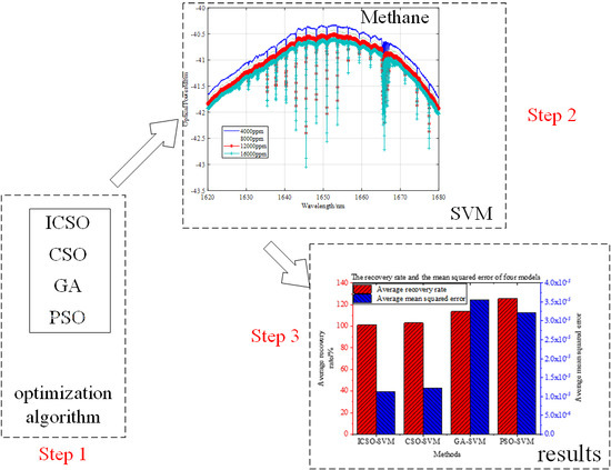
From the 50 train–test repeats experiment, we can see that the recovery rate of ICSO-SVM model shows better stability than other three models. The average recovery rates of ICSO-SVM, CSO-SVM, GA-SVM, and PSO-SVM were 101.23, 103.15, 113.58, and 125.61, respectively. The average mean squared errors of the four models were 1.12 × 10⁻⁵, 1.23 × 10⁻⁵, 3.56 × 10⁻⁵, and 3.22 × 10⁻⁵, respectively. These experimental results verify the feasibility and validity of ICSO-SVM for predicting the concentration of methane.

These are initial steps. Further research should focus on integrating the detection system and algorithm into methane detection equipment, meaning it would be possible to detect methane concentration and obtain a concentration value quickly. Finally, the equipment should be tested at in civil, ambient, and industrial spaces.

References

1. Apte, J.S.; Marshall, J.D.; Cohen, A.J.; Brauer, M. Addressing global mortality from ambient PM2.5. Environ. Sci. Technol. 2015, 49, 8057–8066. [Google Scholar] [CrossRef] [PubMed]
2. Di, Q.; Kloog, I.; Koutrakis, P.; Lyapustin, A.; Wang, Y.; Schwartz, J. Assessing PM2.5 exposures with high spatiotemporal resolution across the continental United States. Environ. Sci. Technol. 2016, 50, 4712–4721. [Google Scholar] [CrossRef] [PubMed]
3. Li, C.; Zhu, Z. Research and application of a novel hybrid air quality early-warning system: A case study in China. Sci. Total Environ. 2018, 626, 1421–1438. [Google Scholar] [CrossRef]
4. Liu, K.; Wang, L.; Tan, T.; Wang, G.; Zhang, W.; Chen, W.; Gao, X. Highly Sensitive Detection of Methane by Near-infrared Laser Absorption Spectroscopy Using A Compact Dense-pattern Multipass Cell. Sens. Actuators B-Chem. 2015, 220, 1000–1005. [Google Scholar] [CrossRef]
5. Cao, Y.; Sanchez, N.P.; Jiang, W.; Griffin, R.J.; Xie, F.; Hughes, L.C.; Zah, C.-E.; Tittel, F.K. Simultaneous Atmospheric Nitrous Oxide, Methane and Water Vapor Detection with A Single Continuous Wave Quantum Cascade Laser. Opt. Express 2015, 23, 2121–2132. [Google Scholar] [CrossRef]
6. Tan, W.; Yu, H.; Huang, C. Discrepant responses of methane emissions to additions with different organic compound classes of rice straw in paddy soil. Sci. Total Environ. 2018, 630, 141–145. [Google Scholar] [CrossRef]
7. Zhou, G. Research prospect on impact of climate change on agricultural production in China. Meteorol. Environ. Sci. 2015, 38, 80–94. [Google Scholar]
8. Contribution of Working Group I to the 5th Assessment Report of the Intergovernmental Panel on Climate Change. The Physical Science Basis; IPCC: Geneva, Switzerland, 2013. [Google Scholar]
9. Shemshad, J.; Aminossadati, S.M.; Kizil, M.S. A review of developments in near infrared methane detection based on tunable diode laser. Sens. Actuators B Chem. 2012, 171, 77–92. [Google Scholar] [CrossRef]
10. Ma, Y.; Lewicki, R.; Razeghi, M.; Tittel, F.K. QEPAS based ppb-level detection of CO and N2O using a high power CW DFB-QCL. Opt. Express 2013, 21, 1008–1019. [Google Scholar] [CrossRef] [PubMed]
11. He, Y.; Ma, Y.; Tong, Y.; Yu, X.; Tittel, F.K. Ultra-high sensitive light-induced thermoelastic spectroscopy sensor with a high Q-factor quartz tuning fork and a multipass cell. Opt. Lett. 2019, 44, 1904–1907. [Google Scholar] [CrossRef] [PubMed]
12. Hao, Z.; Zhao, H.; Zhang, C.; Wang, H.; Jiang, Y.; Yi, Z. Estimating winter wheat area based on an SVM and the variable fuzzy set method. Remote Sens. Lett. 2019, 10, 343–352. [Google Scholar] [CrossRef]
13. Haobin, P.E.N.G.; Guohua, C.H.E.N.; Xiaoxuan, C.H.E.N.; Zhimin, L.U.; Shunchun, Y.A.O. Hybrid classification of coal and biomass by laser-induced breakdown spectroscopy combined with K-means and SVM. Plasma Sci. Technol. 2019, 21, 034008. [Google Scholar] [CrossRef]
14. Tao, Z.; Huiling, L.; Wenwen, W.; Xia, Y. GA-SVM based feature selection and parameter optimization in hospitalization expense modeling. Appl. Soft Comput. J. 2019, 75, 323–332. [Google Scholar] [CrossRef]
15. Wang, X.; Guan, S.; Hua, L.; Wang, B.; He, X. Classification of spot-welded joint strength using ultrasonic signal time-frequency features and PSO-SVM method. Ultrasonics 2019, 91, 161–169. [Google Scholar] [CrossRef]
16. Wang, Y.; Meng, X.; Zhu, L. Cell Group Recognition Method Based on Adaptive Mutation PSO-SVM. Cells 2018, 7, 135. [Google Scholar] [CrossRef]
17. Liu, T.; Liu, S.; Heng, J.; Gao, Y. A New Hybrid Approach for Wind Speed Forecasting Applying Support Vector Machine with Ensemble Empirical Mode Decomposition and Cuckoo Search Algorithm. Appl. Sci. 2018, 8, 1754. [Google Scholar] [CrossRef]
18. He, Z.; Xia, K.; Niu, W.; Aslam, N.; Hou, J. Semi supervised SVM Based on Cuckoo Search Algorithm and Its Application. Mathe. Probl. Eng. 2018, 2018, 8243764. [Google Scholar]
19. Dai, S.; Niu, D.; Han, Y. Forecasting of Power Grid Investment in China Based on Support Vector Machine Optimized by Differential Evolution Algorithm and Grey Wolf Optimization Algorithm. Appl. Sci. 2018, 8, 636. [Google Scholar] [CrossRef]
20. Meng, X.; Liu, Y.; Gao, X.; Zhang, H. A New Bio-Inspired Algorithm: Chicken Swarm Optimization; Advances in Swarm Intelligence; Springer: Berlin, Germany, 2014; pp. 86–94. [Google Scholar]
21. Wu, D.; Kong, F.; Gao, W.; Shen, Y.; Ji, Z. Improved Chicken Swarm Optimization. In Proceedings of the 5th Annual IEEE International Conference on Cyber Technology in Automation, Shenyang, China, 8–12 June 2015. [Google Scholar]
22. Wu, Z.; Yu, D.; Kang, X. Application of improved chicken swarm optimization for MPPT in photovoltaic system. Optim. Control Appl. Meth. 2018, 39, 1029–1042. [Google Scholar] [CrossRef]
23. Liang, J.; Wang, L.; Ma, M.; Zhang, J. A fast SAR image segmentation method based on improved chicken swarm optimization algorithm. Multimed. Tools Appl. 2018, 77, 31787–31805. [Google Scholar] [CrossRef]
24. VAPNIK, V. The Nature of Statistical Learning Theory; Springer: New York, NY, USA, 1995. [Google Scholar]
25. Cherkassky, V. The Nature of Statistical Learning Theory. IEEE Trans. Neural Netw. 1997, 8, 1564. [Google Scholar] [CrossRef] [PubMed]
26. Smola, A.J.; Scholkopf, B. A tutorial on support vector regression. Stat. Comput. 2004, 14, 199–222. [Google Scholar] [CrossRef] [Green Version]
Figure 1. Optimization classification of a hyperplane under a linear condition.
Applsci 09 01761 g001
Figure 2. Structural diagram of methane gas detection system. 1—super light emitting diode light source; 2—condensing mirror; 3, 9—slit; 4, 8, 11—plane mirror; 5—collimator; 6—grating; 7—focus lens; 10—beam splitter; 12, 16, 18, 22—gradient index lens; 13, 14, 19, 20—spherical mirror; 15, 21—air inlet; 17, 23—air outlet.
Applsci 09 01761 g002
Figure 3. The power spectrum of SLED.
Applsci 09 01761 g003
Figure 4. Spectra of four concentrations of methane gas.
Applsci 09 01761 g004
Figure 5. Linear relationship between optical power and methane concentration.
Applsci 09 01761 g005
Figure 6. The fitness curve of improved chicken swarm optimization algorithm.
Applsci 09 01761 g006
Figure 7. The fitness curve of chicken swarm optimization algorithm.
Applsci 09 01761 g007
Figure 8. The fitness curve of genetic algorithm.
Applsci 09 01761 g008
Figure 9. The fitness curve of particle swarm optimization algorithm.
Applsci 09 01761 g009
Figure 10. The relative error percentage for 8test samples.
Applsci 09 01761 g010
Figure 11. The recovery rate of ICSO-SVM.
Applsci 09 01761 g011
Figure 12. The recovery rate of CSO-SVM.
Applsci 09 01761 g012
Figure 13. The recovery rate of GA-SVM.
Applsci 09 01761 g013
Figure 14. The recovery rate of PSO-SVM.
Applsci 09 01761 g014