Experimental Validation of Aero-Hydro-Servo-Elastic Models of a Scaled Floating Offshore Wind Turbine

Abstract

Floating offshore wind turbines are complex dynamical systems. The use of numerical models is an essential tool for the prediction of the fatigue life, ultimate loads and controller design. The simultaneous wind and wave loading on a non-stationary foundation with a flexible tower makes the development of numerical models difficult, the validation of these numerical models is a challenging task as the floating offshore wind turbine system is expensive and the testing of these may cause loss of the system. The validation of these numerical models is often made on scaled models of the floating offshore wind turbines, which are tested in scaled environmental conditions. In this study, an experimental validation of two numerical models for a floating offshore wind turbines will be conducted. The scaled model is a 1:35 Froude scaled 5 MW offshore wind turbine mounted on a tension-leg platform. The two numerical models are aero-hydro-servo-elastic models. The numerical models are a theoretical model developed in a MATLAB/Simulink environment by the authors, while the other model is developed in the turbine simulation tool FAST. A comparison between the numerical models and the experimental dynamics shows good agreement. Though some effects such as the periodic loading from rotor show a complexity, which is difficult to capture.

1. Introduction

The worldwide energy demand is steadily increasing, therefore the supply must follow. Rising greenhouse gas emissions are moving energy suppliers focus heavily towards the renewable energy sector. Wind energy has become a major energy contributor to the renewable energy sector, the global wind capacity in 2018 reached 540 GW [1]. In 2018 a report from the International Energy Agency (IEA) estimated that the wind energy capacity is to increase to between 1700 GW and 2800 GW in 2040 [1], where the offshore wind energy capacity is estimated to be between 160 GW and 350 GW [2]. The wind energy sector is continually moving towards reducing the levelized cost of electricity (LCOE) to make wind energy more competitive with other sources of energy e.g. fossil fuels. Today, offshore wind turbine suppliers are interested in non-conventional offshore wind concepts such as floating foundations. The floating foundation offers the possibility to move the wind turbines out into deeper waters. This opens up for large installation areas where offshore wind turbines was not feasible before. At deep water locations there is often a more steady and continuous wind, which increases the full load hours during the wind turbines lifetime. Furthermore, some concepts of platforms for floating offshore wind turbines (FOWT) offers the possibility to tow out the assembled wind turbine for installation, and also tow it back for maintenance. This could lead to a reduction in installation and maintenance cost.

But FOWTs are complex structures with multiple variables, which all contribute to a highly complex dynamical behavior: Simultaneous wind and wave loads, which are irregular by nature, hydrodynamic and aerodynamic couplings, flexible structures, a non-stationary platform and interaction with electrical components, these all make the design and control of the floating wind turbine a difficult challenge.

To obtain a better understanding of the dynamical behavior of FOWTs there have been extensive research in the area. However, large-scale testing of FOWT are expensive to acquire and operate. Therefore, there has been an increasing focus to use small-scale models which have been experimented on in wave tanks and wind tunnels to validate their numerical models and the design of the structure. A review of some of the projects which addresses the subject of FOWT model validation by use of scaled model experiments is given.

At MARIN, three different 1/50 scaled models were tested by the DeepCWind consortium led by the University of Maine in 2011 and in 2013 [3,4]. The test was part of a model test campaign, which were to produce experimental data which could be used for validating offshore wind modeling tools. The FAST code has been calibrated and validated with use of these data [5,6]. The initial tests in 2011 were on a Tension-Leg Platform (OC-4 TLP), semi-submersible (OC4-semi) platform and a spar-buoy (OC4-spar). These platforms used a rotor which was based on Froude scaling of the NREL 5 MW wind turbine. The platforms were tested in simultaneous wind and wave environments. Due to the geometrically scaled rotor, the Reynolds number was not scaled; as a consequence the aerodynamic performance not match the scaled aerodynamic performance. In 2013, a new rotor was developed, this was designed to replicate the aerodynamic loads of the 5 MW NREL wind turbine and a scaled flexible tower was designed. This new rotor and tower were mounted on the previously used OC4-semi platform from 2011 and retested. These tests showed that the scaled aerodynamic properties was better matched.

In 2015, a 1/60 scaled model of a 10 MW wind turbine was developed to match the scaled rotor thrust and the OC-4 semi platform was modified to support this [7]. The scaled model was tested in different scaled operational conditions with simulations wind and wave loads and under extreme load conditions. In addition, a feedback controlled ducted fan was used to simulate the thrust force in some of the experiments.

At Kyushu University, three platform designs for a 1/100 scaled model 2 MW wind turbine was tested without any aerodynamic loading in 2009 [8]. The experimental results were compared to the numerical predictions where potential theory and Morison’s equation was used. These results showed that one of the designs, a stepped cylindrical shaped platform, was promising. This led to larger 1/22.5 scaled model of the stepped cylindrical shaped platform which was tested in the deep-sea wave basin at National Maritime Research Institute in 2009 [9]. To simulate the aerodynamic loading from the rotor a steady horizontal force was applied by a constant weight on a pulley. The experimental results showed good agreement with the numerical simulations and no unexpected phenomenon was observed. A 1/10 scaled model of the stepped cylindrical shaped platform was deployed at sea in 2010 [10]. The feasibility of the hybrid-spar concept was confirmed through the study which lead to a half-scale prototype in 2011 [11] and full-scale prototype in 2013 which was also installed and tested at sea. The numerical simulations during power production showed good agreement and both prototypes even survived several severe typhoons [12].

At the University of California, Berkeley a feasibility study of the triangular semi-submersible platform Windfloat was conducted in 2010 [13]. This were done by using a 1/100 scaled platform for a 5 MW wind turbine. The platform was tested in a wave basin. The aerodynamic thrust and the gyroscopic force were simulated by an actuator disk and a scaled spinning mass respectively.

The spar platform concept from HyWind was tested at Marintek in 2005 on a 1/47 scaled model of a 5 MW wind turbine [14,15]. The tests were done in combined wind and wave conditions. The rotor was Froude scaled and its speed was set by a dc-motor which was controlled to obtain the right power. The collective blade pitch was controlled by another DC-motor. At the technical university of Denmark, a 1/60 model of the 10MW DTU reference wind turbine mounted on a TLP platform was tested in 2015 [16,17]. The tests were done in scaled wind and wave conditions, with a Froude scaled rotor. A later study used a redesigned rotor, which was designed to match the scaled rotor thrust [18]. A later study in 2017 used a new platform, which was, the triple spar platform, which is a hybrid between a spar buoy and a semi-submersible tri-floated concept which had been developed at DTU. The scaled model was tested in a range of wind-wave conditions and with different control strategies. The main focus was the effects of aerodynamic damping and interaction effects between the wind forcing, wave forcing and the blade pitch control algorithm.

At the university Ecole Centrale de Nantes a 1/60 scaled model of an upscaled 6 MW wind turbine, on the concrete star wind platform, was tested in 2013 [19]. This platform is a braceless-semisubmersible platform design, the wind turbine thrust was upscaled from the 5 MW NREL wind turbine and was generated by a controllable ducted fan at the top of the tower. The thrust was controlled by adjusting the rotational speed of the fan, which was set by a reference from a real-time simulation of the scaled model in FAST.

The contribution of this paper is the experimental validation of two numerical simulation models for the new FOWT design: the AAUE-TLP. The scaled floating wind turbine model used in this paper is referred to as AAUE-TLP. These simulation models can be used as baseline models for future studies. The simulation models will be validated in several experiments with wind and wave loads applied. The theory for developing a coupled aero-hydro-servo-elastic model for a FOWT is presented in this paper. Furthermore, to do a code-to-code comparison, the FAST model is calibrated for the AAUE-TLP. The design of AAUE-TLP differs from other state-of-the-art scaled FOWT models by being a large-sized scaled model, which have an individual blade pitch system. This will be advantageous in future studies of control methods for FOWTs as individual pitch control can be applied. The blades of the wind turbine are designed to match the Froude scaled thrust, but at a larger wind speed interval. This will make the wind turbine less sensitive to wind speed variations in the wind field. The FAST code for the scaled floating offshore wind turbine AAUE-TLP can be downloaded from [20].

In this paper the simulations and experiments are compared in two DOF. These two DOF are the TLPs and tower top surge movement because these are the most dominant DOFs.

The paper is organized as follows: The theoretical aero-hydro-servo-elastic model is presented in Section 2. The experimental setup is described in Section 3. The theoretical model verification is conducted in Section 4. The conclusions are made in Section 5.

2. Aero-Hydro-Servo-Elastic Model

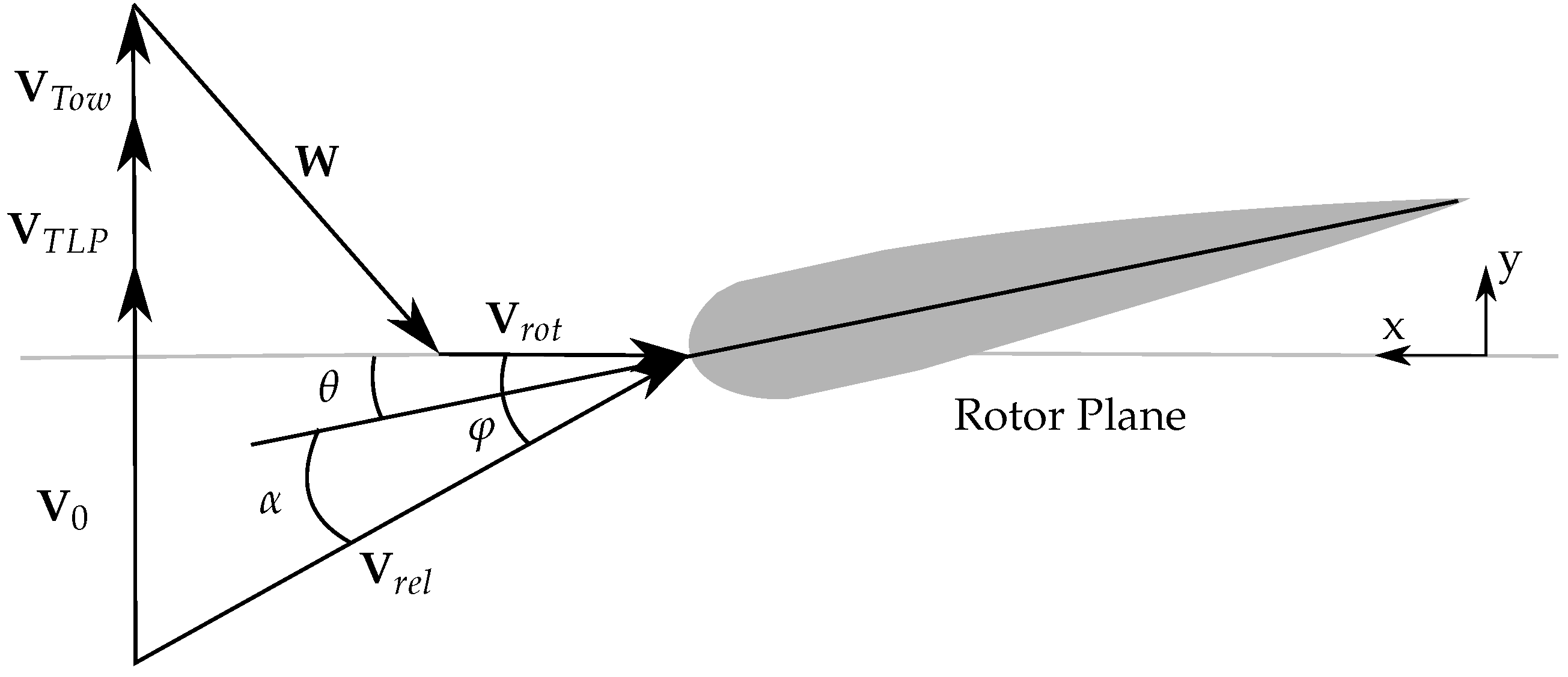
2.1. Aerodynamic Model

To model the transient rotor loading for a FOWT the unsteady Blade Element Method (UBEM) is used. The unsteady flow around a FOWT is caused by different factors. The factors which are taken into account in this paper are the unsteady and uneven wind field with turbulence, the translational velocity of the TLP and tower. The structural dynamics of the blade are not taken into account, as this is assumed to be small compared to the surge motion. Furthermore, the yaw motion of the wind turbine is not taken into account in the aerodynamic calculations. The theory presented in this paper regarding the modeling of unsteady aerodynamics of wind turbines is mainly by M. Hansen from [21]. The BEM arises from a combination of two theories; the 2D blade element theory and the 1D momentum theory. In BEM the blade is discretized spanwise, and the forces are calculated for each section, which is summarized at the end to calculate the forces on the whole rotor. To model the unsteady effects in BEM three unsteady dynamic models are applied, these are a dynamic stall model, a dynamic inflow model, and a tower-interference model.

The main objective of the BEM method is to calculate the relative velocity the blade sections experience. The relative velocity at a blade section can be found by

$${\mathbf{V}}_{rel}={\mathbf{V}}_0+{\mathbf{V}}_{Tow}+{\mathbf{V}}_{TLP}+{\mathbf{V}}_{Rot}+\mathbf{W}$$

(1)

where ${\mathbf{V}}_{rel}\in {\mathbb{R}}^2$ is the relative velocity at a blade section, ${\mathbf{V}}_0\in {\mathbb{R}}^2$ is the free stream velocity of the wind, ${\mathbf{V}}_{TLP}\in {\mathbb{R}}^2$ and ${\mathbf{V}}_{Tow}\in {\mathbb{R}}^2$ is the translational velocity of the TLP and tower respectively, ${\mathbf{V}}_{Rot}\in {\mathbb{R}}^2$ is the rotational velocity at the blade section and W is the induction velocity. The velocity vectors can be visualized in Figure 1.

The flow angle can be found from the two components of the relative wind speed. By a geometrical inspection of the velocity triangle, the flow angle can be calculated as

$$tan\left(\varphi \right)=\frac{{\mathbf{n}}_y{\mathbf{V}}_{rel}}{-{\mathbf{n}}_x{\mathbf{V}}_{rel}}$$

(2)

where $\varphi$ is the flow angle, ${\mathbf{n}}_y$ and ${\mathbf{n}}_x$ are the direction vectors vectors ${\mathbf{n}}_y$ = [0 1] and ${\mathbf{n}}_x$ = [1 0]. From this the blades angle of attack can be found as

$$\alpha =\varphi -(\beta +\theta )$$

(3)

where $\beta$ is the blade sections pitch angle and $\theta$ is the blade sections geometrical twist. As the yaw movement of the wind turbine is neglected, the induced velocity can be described by two induction factors

$$a={\left(\frac{4F{sin}^2\left(\varphi \right)}{\nu C_n}+1\right)}^{-1}$$

(4)

$$a^{\prime }={\left(\frac{4Fsin\left(\varphi \right)cos\left(\varphi \right)}{\nu C_t}-1\right)}^{-1}$$

(5)

where a and a′ are the axial and tangential induction factors respectively. $\nu$ is the solidity factor, which describes the fraction of the blade section covers in the rotor annulus. F is Prandtl’s tip loss factor, which describes the loss from the tip wake at the blade section. $C_n$ and $C_t$ are the normal and tangential coefficients. These are found by the projection of the lift and drag coefficients, which can be found by using airfoil data for a given angle of attack. The expression for the axial coefficient in Equation (4) hold for values lower than approximately 0.2, as beyond this the momentum theory does no longer hold, therefore the Glauert’s correction is used in this case.

The tangential and normal force on the blade section can be calculated as

$$F{T}_{j,k}=\frac{1}{2}{\rho }_a{\mathbf{n}}_1{\mathbf{V}}_{rel}{C}_{t}cdr$$

(6)

$$F{N}_{j,k}=\frac{1}{2}{\rho }_a{\mathbf{n}}_2{\mathbf{V}}_{rel}{C}_{n}cdr$$

(7)

where $FT$ and $FN$ are the tangential and normal force on blade j, at blade section, k. ${\rho }_a$ is the density of the air. c and $dr$ is the chord length and spanwise length of the blade section respectively.

It is clear that these equations must be solved iteratively since the flow angle and thus also the angle of attack depends on the induced velocity itself. But as this method is unsteady, the time is here used as a relaxation. Therefore, the simulation time step is set to 0.05 s. Thereby, the induced velocity vector calculated from the previous timestep is used for the current timestep. This can be accomplished as the induced velocity changes relatively slow in time compared to the simulation time step. This is incorporated in the simulation model by using a dynamic wake model. In this paper, the TUDK dynamic wake model from S. Oye given in [22] is used. The angle of attack will not change instantaneously, but instead with a time delay. To model this a dynamic stall model from S. Oye given in [23] is used to model the angle of attacks dynamic change. At last the tower shadow model from M. Hansen given in [21] is used to describe the effect of the tower on the incoming wind speed.

2.2. Hydrodynamic Model

The hydrodynamic model used in this project is the same as previously used and described in [24], see this for more information. To model the movement of the TLP in six DOF in the time domain, a modified version of Cummin’s equation [25] is utilized. The movement of a rigid floating structure was described by W.E Cummins by a second order differential equation with a convolution integral. The model is modified by incorporating a linear and quadratic viscous damping term into Cummin’s equation yielding a linear vector integro differential equation

$$\begin{array}{c}\left({\mathbf{M}}_{TLP}+\mathbf{A}(\infty )\right)\ddot{\mathbf{y}}\left(t\right)+{\int }_0^z{\mathbf{B}}_{quad,v}\left((\mathbf{u}(t,z)-\dot{\mathbf{y}}(t,z))\left|\mathbf{u}(t,z)-\dot{\mathbf{y}}(t,z)\right|\right)dz\hfill \\ +{\int }_0^z{\mathbf{B}}_{lin,v}(\mathbf{u}(t,z)-\dot{\mathbf{y}}(t,z))dz+{\int }_0^t\mathbf{R}(t-\tau )\dot{\mathbf{y}}\left(\tau \right)d\tau +{\mathbf{K}}_{\mathbf{TLP}}\mathbf{y}\left(t\right)={\mathbf{F}}_{wave}\left(t\right)\hfill \end{array}$$

(8)

where $\ddot{\mathit{y}}$, $\dot{\mathit{y}}$ and $\mathit{y}$, denote the acceleration, velocity and position of the TLP, respectively in ${\mathbb{R}}^6$. $\mathbf{u}\in {\mathbb{R}}^6$ denotes the velocity of the water particles, which decays exponentially towards the bottom. The viscous forces arising from the relative velocity therefore needs to be integrated along the height of the TLP. ${\mathbf{M}}_{TLP}\in {\mathbb{R}}^{6\times 6}$ is the inertia matrix of the TLP. $\mathbf{A}(\infty )\in {\mathbb{R}}^{6\times 6}$ is a constant positive-definite added mass matrix at an infinite frequency. ${\mathbf{B}}_{lin,v}$ and ${\mathbf{B}}_{quad,v}$ denote the linear and quadratic viscous damping matrices respectively both in ${\mathbb{R}}^{6\times 6}$. The linear and quadratic viscous damping matrices are found by analyzing experimental data from the free decay motion of the TLP, the data for this can be seen in [24]. ${\mathbf{K}}_{\mathbf{TLP}}\in {\mathbb{R}}^{6x6}$ is the combined stiffness matrix from the hydrostatic stiffness and mooring stiffness. The hydrostatic stiffness arises due to changes in the water-plane area and the interaction between the forces from gravity and buoyancy, this is described in [26]. The mooring stiffness is found by analytical force/moments equilibrium as described in [27]. ${\mathbf{F}}_{wave}\in {\mathbb{R}}^6$ describes the wave induced forces and moments on the TLP, in this paper only the first order wave forces are taken into account. $\mathbf{R}\in {\mathbb{R}}^{6x6}$ is a matrix consisting of retardations functions, which describe the radiation impulse responses in the different DOFs. The radiation impulse response can be described in the time domain as

$$\mathbf{R}\left(t\right)=\frac{2}{\pi }{\int }_0^{\infty }{\mathbf{B}}_{pot}\left(\omega \right)cos\left(\omega t\right)d\omega$$

(9)

where the retardation function is a conversion of the frequency dependent potential damping matrix ${\mathbf{B}}_{pot}\left(\omega \right)\in {\mathbb{R}}^{6\times 6}$ from the frequency domain to the time domain through the Fourier transform. This effect captures the energy transfer from the motion of the structure to the surrounding fluid. The hydrodynamic coefficients $\mathbf{A}(\infty )$, ${\mathbf{B}}_{pot}\left(\omega \right)$ and the wave height normalized frequency dependent first order wave loads ${\overline{\mathbf{F}}}_{wave}\left(\omega \right)$ are calculated by solving the velocity potential of the diffraction problem when appropriate boundary conditions are applied. This is done by loading the geometry of the TLP into the software NEMOH [28], which uses the boundary element method to solve the diffraction problem. The convolution integral formulation in Equation (8), describes the change in the fluid momentum due to the motion of the structure at a particular time instant, which will affect the motion of the structure at all subsequent times. The convolution integral formulation requires a significant amount of computer memory if directly implemented. Therefore, in this paper, the convolution integral formulation is approximated by a linear state-space model, as described in [29]. The linear state-space model that describes the memory effect is created by using the MSS FDI [30] toolbox in MATLAB. The MSS FDI toolbox uses system identification to paramitize the state-space model based on the non-parametric retardation functions. Thereby, the convolution integral can be approximated by a state space model as

$$\mu ={\int }_0^{\infty }\mathbf{R}(t-\tau )\dot{\mathbf{y}}\left(\tau \right)d\tau \Rightarrow \left\{\begin{array}{c}\dot{\mathbf{x}}={\mathbf{A}}_c\mathbf{x}+{\mathbf{B}}_c\dot{\mathbf{y}}\hfill \\ \mathit{\mu }={\mathbf{C}}_c\mathbf{x}\hfill \end{array}\right.$$

(10)

where the matrices ${\mathbf{A}}_c$, ${\mathbf{B}}_c$ and ${\mathbf{C}}_c$ are time invariant and the number of components in the state vector x corresponds to the order of the approximated model.

2.3. Drive Train Model

To model the rotational energy transfer from the rotor to the generator through a gearing, a drive train model is used. The drive train model is modeled on the low speed shaft side, by Newton’s second law for rotation of a rigid body SDOF system

$$N_G{T}_g-T_r=J_{dt}{\dot{\omega }}_r+B_{dt}{\omega }_r+T_0$$

(11)

where the DOF is the angular rotation of the low speed shaft. $N_G$ is the high speed to low speed gear ratio, $T_g$ is the generator torque on the high speed shaft. $J_{dt}$ is the equivalent drive train mass moment of inertia w.r.t the low speed shaft, ${\omega }_r$ is the rotor velocity and ${\dot{\omega }}_r$ is the rotor acceleration. $B_{dt}$ is the dynamic friction for the main shaft also known as viscous friction. $T_0$ is a combination of the torque contributions from the static friction, coulomb friction and the detent torque, all of them opposing the motion at standstill.

2.4. Tower Modelling

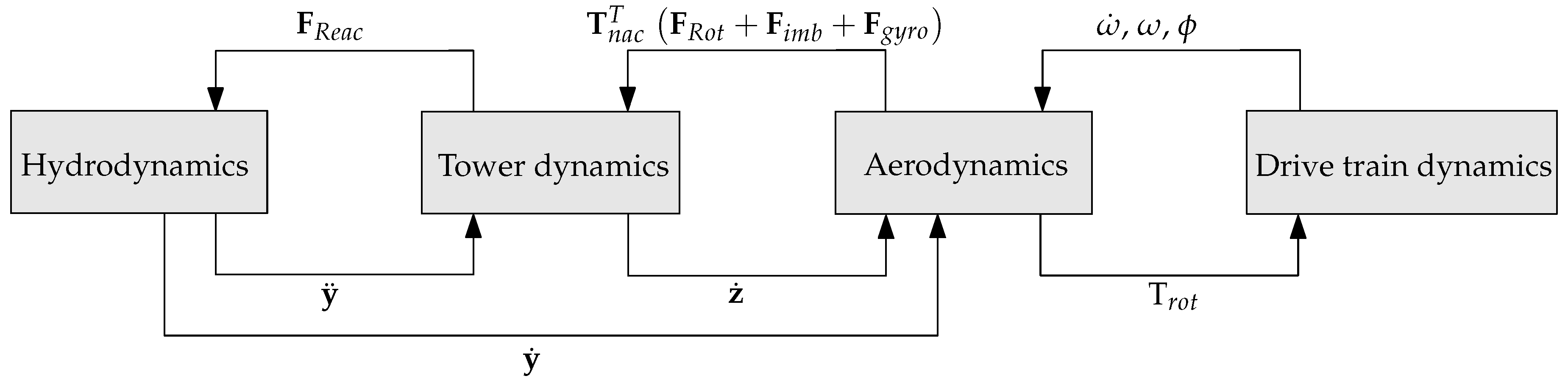
The tower model used in this project is the same as previously used and described in [24] see this for more information. The towers and nacelles dynamics are described by a Finite Element Model (FEM) constructed in a MATLAB code. The FEM model is based on an assembly of 3D beam elements each with 6 DOF. The FEM of the structure of the tower consists of 20 nodes along the tower and 2 nodes for the nacelle. Each node has six DOFs, and between two nodes are an element. The governing equation for one element, can be described by a mass-spring-damper system

$${\mathbf{m}}_{tow}\ddot{\mathbf{z}}+{\mathbf{c}}_{tow}\dot{\mathbf{z}}+{\mathbf{k}}_{tow}\mathbf{z}=\mathbf{f}$$

(12)

where $\ddot{\mathbf{z}}\in {\mathbb{R}}^6,\dot{\mathbf{z}}\in {\mathbb{R}}^6$ and $\mathbf{z}\in {\mathbb{R}}^6$ is the acceleration vector, velocity vector and position vector, respectively. ${\mathbf{m}}_{tow}\in {\mathbb{R}}^{6\times 6}$ is the mass matrix of a single element, ${\mathbf{c}}_{tow}\in {\mathbb{R}}^{6\times 6}$ is the damping matrix, ${\mathbf{k}}_{tow}\in {\mathbb{R}}^{6\times 6}$ is the stiffness matrix, and $\mathbf{f}\in {\mathbb{R}}^6$ is the vector describing the external force applied to each DOF.

For the mass matrix of the elements, a combination of the lumped mass matrix and consistent mass matrix is chosen. The derivation can be found in several textbooks e.g., [31]. The combinational mass matrix is chosen as it tends to estimate the natural frequency better, than the use of a single one of the latter two mass matrix formulations [31]. The combinational mass matrix is written as

$${\mathbf{m}}_{tow}={\mathbf{m}}_{Lump}\gamma +{\mathbf{m}}_{Con}(1-\gamma )$$

(13)

where ${\mathbf{m}}_{Lump}$ and ${\mathbf{m}}_{Con}$ is the lumped mass matrix and consistent mass matrix, respectively. $\gamma$ is a weighting parameter which takes a value between 0 and 1, in this paper a value of 0.5 is found suitable. The mass of the tower is formulated such that it is equally distributed along its longitudinal axis, whereas the mass of the nacelle and rotor is formulated to be placed in the center node of the nacelle.

For the stiffness matrix of the elements a 3D beam formulation is utilized, for more information see [32]. The bending-transverse stiffness of the elements consist of two stiffness components; the bending stiffness and initial stress stiffness. The bending stiffness is described by Bernoulli-Euler beam theory, which is a good approximation for long slender structures, such as the tower of the AAUE-TLP. The initial stress stiffness arises due to the weight of the wind turbine and tower, this decreases the stiffness of the structure. The axial and twisting motion is assumed to small, and thereby their motion can assumed to be decoupled. Thereby the axial and twisting stiffness of the elements can be formulated as linear spring by Hook’s law. The tower used in this paper have a symmetric cross section, this makes the decoupling of bending, axial and twisting motion a valid assumption [33]. For the damping matrix of the elements a classical Rayleigh damping formulation is used. Rayleigh damping is a viscous damping model, where the damping matrix is assumed to be a linear combination of the mass and stiffness matrices, which can be written as

$${\mathbf{c}}_{tow}={\alpha }_d{\mathbf{m}}_{tow}+{\beta }_d{\mathbf{k}}_{tow}$$

(14)

where ${\alpha }_d$ and ${\beta }_d$ are two weighting parameters. To determine the value of the weighting parameters in this paper, the damped natural frequency and the corresponding damping ratio are used. These are found by analyzing data from free decay tests of the tower mounted on the TLP, the mean damping ratio was found to be 0.025 and a damped natural frequency of 1.72 Hz. In this paper, the first natural frequency and damping ratio were found by free decay experiments. From these experimens the two weighting parameters can be determined by

$${\alpha }_d={\zeta }_1{\omega }_1\mathrm{and}{\beta }_d=\frac{{\zeta }_1}{{\omega }_1}$$

(15)

where ${\alpha }_d$ and ${\beta }_d$ can be calculated to be 0.270 and 0.002, respectively. The Rayleigh damping model is an approximation of the damping matrix and is often used for its ease of implementation. Furthermore, the mass proportional term will dampen the low frequency motions heavily, while the stiffness proportional term will dampen the high frequency motion heavily. In the simulations, a non-physical high frequency motion can occur, the stiffness proportional damping will also help dampen these [31].

To describe the motion of the tower structure, the local elements must be assembled into a global formulation. The local system matrices are converted into global system matrices, which give the global governing equation for the tower

$${\mathbf{M}}_{tow}\ddot{\mathbf{Z}}+{\mathbf{C}}_{tow}\dot{\mathbf{Z}}+{\mathbf{K}}_{tow}\mathbf{Z}={\mathbf{F}}_{ext}$$

(16)

where $\ddot{\mathbf{Z}}\in {\mathbb{R}}^{6N}$, $\dot{\mathbf{Z}}\in {\mathbb{R}}^{6N}$ and $\mathbf{Z}\in {\mathbb{R}}^{6N}$ is the global acceleration vector, velocity vector and position vector, respectivly, N is the number of nodes used for the tower and wind turbine discretization, which in this paper is 22. ${\mathbf{M}}_{tow}\in {\mathbb{R}}^{6N\times 6N}$ is the global mass matrix, ${\mathbf{C}}_{tow}\in {\mathbb{R}}^{6N\times 6N}$ is the global damping matrix, ${\mathbf{K}}_{tow}\in {\mathbb{R}}^{6N\times 6N}$ is the global stiffness matrix. ${\mathbf{F}}_{ext}\in {\mathbb{R}}^{6N}$ is the global load vector on the tower structure. At the top two elements, which is the wind turbine, the mass and inertia were found by usage of the 3D-model developed in the 3D CAD software Inventor [34]. The stiffness of the nacelle is assumed to be from the rectangular plate, the stiffness is therefore modeled as a rectangular plate of aluminum. The damping is assumed to be the same as used for the tower.

2.5. Coupling Model

The theoretical models for the different subsystems of the FOWT are explained in the above subsections. In order to simulate the coupled dynamics, the coupling between the subsystems must be described. A visualization of the coupling between the different subsystems can be seen in Figure 2.

The TLP is considered as a moving support for the tower. The effect of the moving support from the TLP to the tower can be described by a force in each node. This force can be can be described by assuming that the acceleration of the TLP is applied to all nodes in their respective DOF [35]. The force vector can then be calculated by using Newton’s second law

$${\mathbf{F}}_{sup}={\mathbf{T}}_{tow}{\mathbf{M}}_{tow}\ddot{\mathbf{y}}$$

(17)

where ${\mathbf{F}}_{sup}\in {\mathbb{R}}^{6N}$ is the force vector arising from the acceleration of the TLP on the tower. ${\mathbf{M}}_t\in {\mathbb{R}}^{6N\times 6N}$ is the global mass matrix for the tower and nacelle. $T_{tow}\in {\mathbb{R}}^{6Nx6}={[{\mathbf{I}}_{6x6}{\mathbf{I}}_{6x6}\dots {\mathbf{I}}_{6x6}]}^T$ is a transformation matrix consisting of N-identity matrices. This transforms the TLPs accelerations into each of the nodes FEM model of the tower, in the respective DOFs.

The towers relative movement with respect to the TLP will also affect the TLPs movement. The reaction force can be calculated in the bottom node of the FEM model of the tower and applying it to the TLPs external forces. The reaction force can be calculated by

$${\mathbf{F}}_{Reac}=\left({\mathbf{C}}_{tow}\dot{\mathbf{Z}}+{\mathbf{K}}_{tow}6\mathbf{Z}\right){\mathbf{T}}_{Reac}$$

(18)

where ${\mathbf{F}}_{Reac}\in {\mathbb{R}}^6$ is the reaction force in the bottom node of the FEM of the tower. ${\mathbf{T}}_{Reac}\in {\mathbb{R}}^{6\times 6N}$ is a transformation matrix, which transforms the global load matrix from the FEM model of the tower to the load matrix for the TLP. The motion of the TLP and tower will affect the rotors aerodynamics by changing the wind speed the wind turbines blades experience. The TLP and towers motion in surge are taken into account for the relative wind speed in Equation (1). The loads from the aerodynamics on the rotor in this paper are the rotor thrust force and moments in pitch and yaw, and a roll moment around the tower is due to the acceleration of the rotor. These loads will be inserted as an external force on the center node of the nacelle in their respective DOF in the FEM code for the tower. The loads arising from the rotor are

$${\mathbf{F}}_{Rot}={\left[\begin{array}{cccccc}{F}_{Su}& 0& 0& M_{Ya}& M_{Pi}& M_{Ro}\end{array}\right]}^T$$

(19)

where ${\mathbf{F}}_{Rot}\in {\mathbb{R}}^6$ is the load vector from the rotor. $F_{Su}$ are the thrust force on the rotor. $M_{Pi}$ and $M_{Ya}$ are the pitch and yaw moment around the tower. These load components from the aerodynamics can be calculated as

$$F_{Su}=\sum _{j=1}^{NB}\sum _{k=1}^{NS}{FT}_{j,k}$$

(20)

$$M_{Pi}=\mathbf{Si}\mathbf{FT}\mathbf{Br}$$

(21)

$$M_{Ya}=\mathbf{Co}\mathbf{FT}\mathbf{Br}$$

(22)

where $\mathbf{FT}\in {\mathbb{R}}^{NB\times NS}$ are the thrust force matrix. $NS$ is the number of blade sections used in the unsteady BEM model and $NB$ is the number of blades. In this paper, the blade is split into 19 blade sections on each of the 3 blades. $\mathbf{Br}\in {\mathbb{R}}^{NS}$ is a distance vector, which describes the blades spanwise length from center to each of the blade sections. Si = [$sin\left({\varphi }_r\right)sin({\varphi }_r+2\pi /3)sin({\varphi }_r+4\pi /3)$] and Co = [$cos\left({\varphi }_r\right)cos({\varphi }_r+2\pi /3)cos({\varphi }_r+4\pi /3)$], where ${\varphi }_r$ is the reference blades azimuthal postion.

The roll moment induced around the tower top can be calculated as

$$M_{Ro}=3{\dot{\omega }}_r{\mathbf{Br}}^T\mathbf{mr}$$

(23)

where $M_{Ro}$ are the roll moment around the tower. $\mathbf{mr}\in {\mathbb{R}}^{NS}$ is the blade mass vector, consisting of the mass of the individual blade the blade sections. The blades of the wind turbine in this paper have a slightly mass inequality, therefore the center of mass of mass of the rotor will be slightly shifted from the geometric center of the rotor. In this paper the center of mass is only considered to be shifted in the rotor plane, this will cause the center of mass of the rotor to take a cyclical path in the rotor plane. The force arising from the mass imbalance is modeled by considering one blade to have a reference mass, and the two other blades to have an equal mass imbalance in opposite directions. The reference mass is taken as mean weight of the blades, which is 0.76 kg, while the mass imbalance is approximated to be 5% of the reference mass, which is ±0.04 kg. The force from the rotor mass imbalance is caused by the centrifugal force, which can be calculated as

$${\mathbf{F}}_{imb}=\sqrt{3}{m}_{b,imb}{r}_{b,cm}{\omega }_r^2{\mathbf{T}}_{imb}^T$$

(24)

where ${\mathbf{F}}_{imb}\in {\mathbb{R}}^6$ is the mass imbalance force vector. $m_{b,imb}$ is the blades mass imbalance, which is set to 0.04 kg. $r_{b,cm}$ is the distance from the center of the rotor to the center of mass of the blades, which is set to 0.4 m. The imbalance force acts in sway and heave dependig in the azimuthal position of the mass imbalance, which here is set to be at the reference blades position, so ${\mathbf{T}}_{imb}$ = [ 0 $sin\left({\varphi }_r\right)cos\left({\varphi }_r\right){\mathbf{O}}_{1x3}$]. In this paper, an aerodynamic imbalance between the blades is also taken into account. The aerodynamic imbalance might be due to the fabrication errors of the blades, an offset in the calibration of the blade encoders or measurement errors from the blade encoders. A gyroscopic force arises when the TLP or tower either moves in pitch or yaw and thereby change the rotor plane. When changing the spinning rotors plane, a gyroscopic force arise which will couple the yaw and pitch motion. The gyroscopic force vector can be found as

$${\mathbf{F}}_{gyro}={\omega }_r{J}_r\left[\begin{array}{cc}{\mathbf{O}}_{4x4}& {\mathbf{O}}_{4x2}\\ {\mathbf{O}}_{2x4}& \mathbf{B}\end{array}\right]\left({\mathbf{T}}_{nac}\dot{\mathbf{Z}}+\dot{\mathbf{y}}\right)$$

(25)

where ${\mathbf{F}}_{gyro}\in {\mathbb{R}}^6$ is the gyroscopic force vector. $J_r$ is the mass moment of inertia of the rotor. ${\mathbf{T}}_{nac}$ = [${\mathbf{O}}_{6x6(N-2)}{\mathbf{I}}_{6x6}{\mathbf{O}}_{6x6}$] is a transformation matrix which isolates the center node of the nacelle in the FEM of the tower and nacelle. B = $\left[\begin{array}{cc}0& -1\\ 1& 0\end{array}\right]$ is a matrix coupling the roll and yaw motion.

The rotor aerodynamics will also couple with the drivetrain as the rotors aerodynamic torque will affect the drive train torque balance as seen in Equation (11). The drive train will affect the rotor aerodynamics by the rotational acceleration, speed and position of the rotor.

2.6. FAST

The numerical simulation software FAST (Fatigue, Aerodynamics, Structures, and Turbulence) developed by NREL [36], is a aeroelastic computer-aided engineering tool for simulating coupled dynamic response of wind turbines. In this paper FAST V8 is utilized. FAST combines the theories for hydrodynamics, aerodynamics, structural elastic dynamics, electrical systems and control system into one coupled non-linear aero-hydro-servo-elastic simulation in time domain. FAST is based on severeal sub-modules for the different dynamics, in this paper the following packages are utilized; Elastodyn for the tower dynamics, AeroDyn for calculation of the aerodynamics on the wind turbine, Inflowwind for specifing the wind field, HydroDyn for calculation of the hydrodynamics loads on the TLP, ServoDyn for implementing the simulink model of the drive-train, actuators and control system, SubDyn for modelling the coupling between structural members and FEAMooring for modelling the mooring dynamics. For more information about the FAST setup and parameters, see [24].

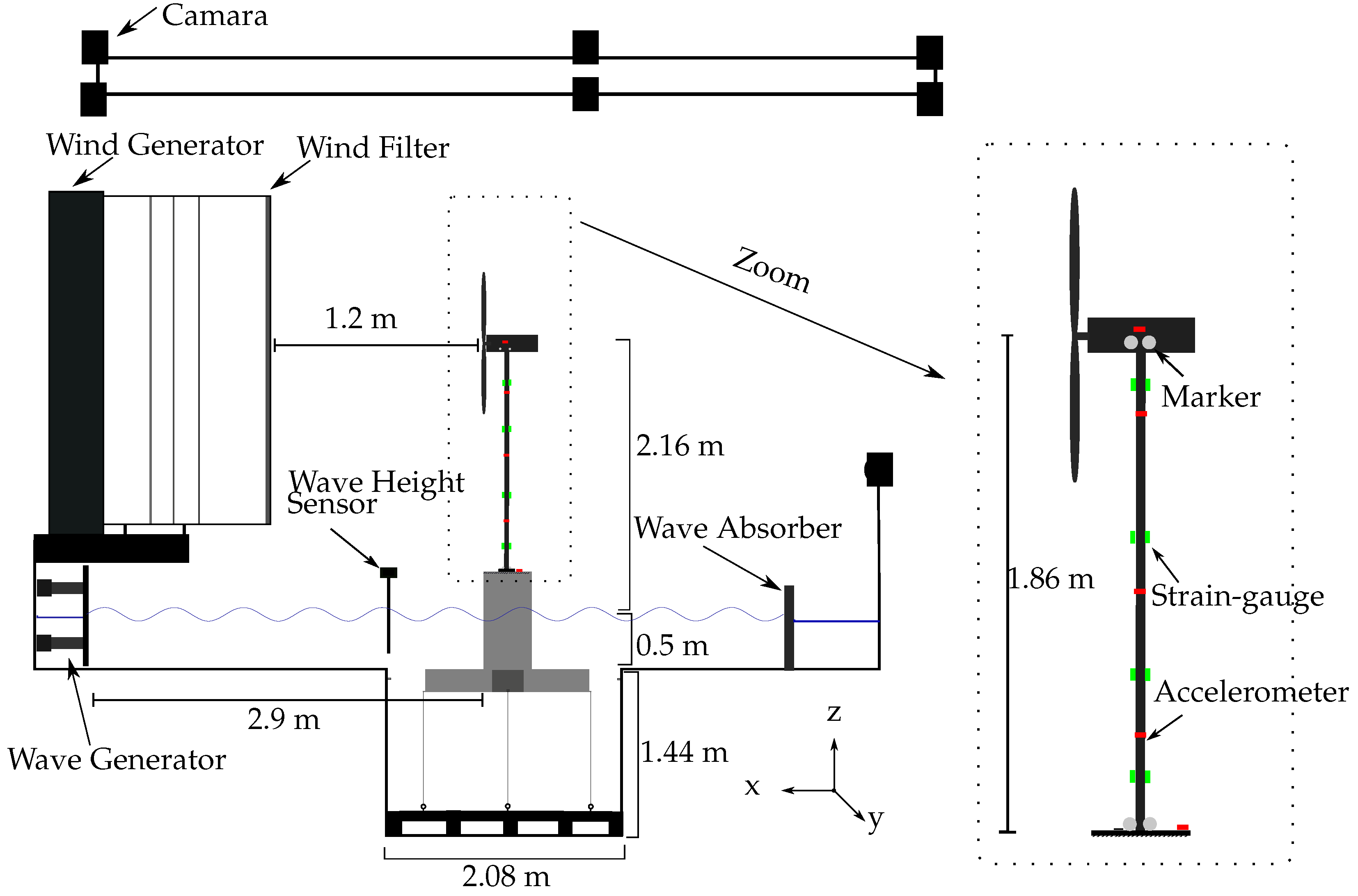
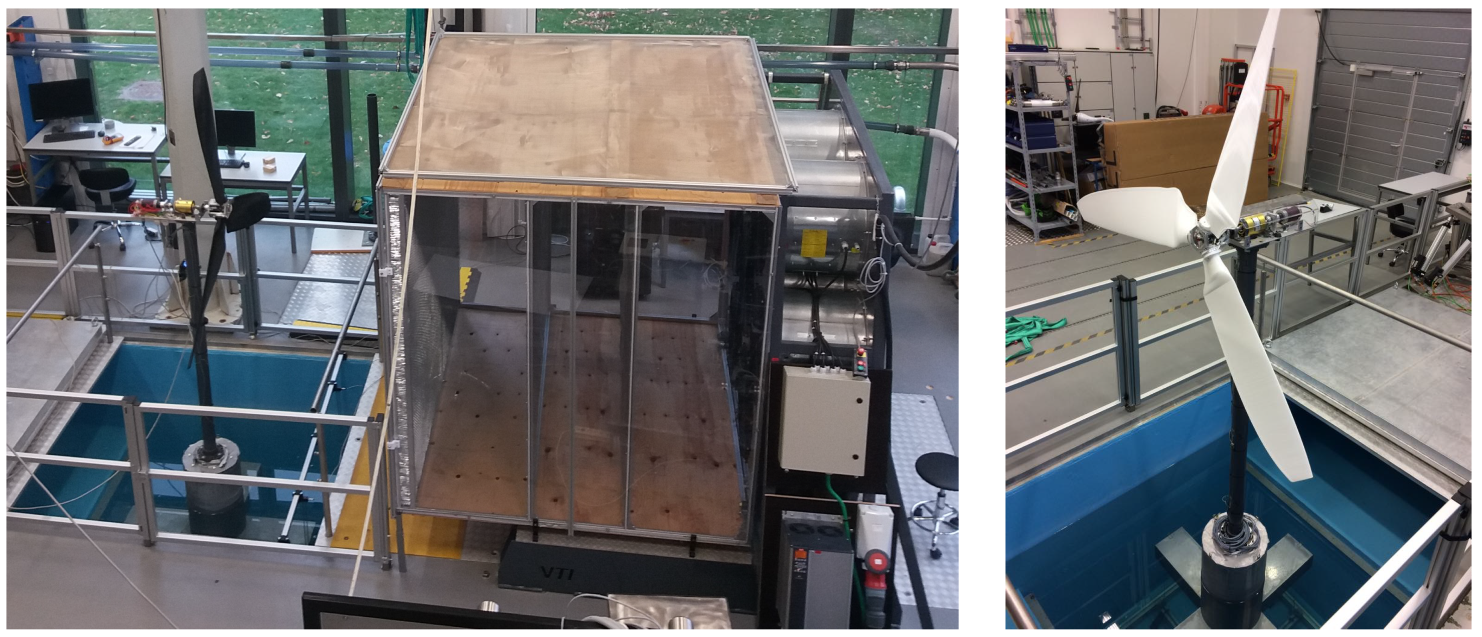
3. Experimental Setup

In this paper, the laboratory facilities used to test the scaled model of the FOWT is a wind generator with a wind filter in front of it, a wave tank with a wave generator and a camera tracking system. A visualization of the whole laboratory setup can be seen in Figure 3.

The wind and wave generator are installed such that the wind and wave generated are aligned. The wind generator consists of seven fans which are placed in a circular pattern. Each fan have a rated power of 4 kW. The rotational speed of fans can be controlled by an inverter, such that different wind speeds can be generated. The wind speeds which can be generated are up to 9 m/s. In front of the wind generator, a wind filter is mounted, this is designed to reduce the turbulence of the wind, straighten the wind flow, and make the wind field more uniform. The wind filter consists of three reconfigurable mesh screens, with different mesh sizes and a honeycombs screen at the outlet. The wind filter outlet have an height of 2.2 m and a width of 2.4 m. The wave tank is constructed with a shallow water depth, except at the middle where a pocket is made, which is also where the TLP is anchored to in the bottom. The wave generator is a piston type with a stroke length of 0.7 m, which is controlable through the software AwaSys [37]. It is able to generate unidirectional linear waves in the frequency range of approx. 0.2 Hz to 2 Hz. The wave generator can be set to generate regular waves, but also irregular waves according to a given wave spectrum. At the ends of the wave basin a passive wave absorber is placed, to minimize reflections.

To track the movement of the TLP and tower top, an infrared camera system Prime 13 from OptiTrack was utilized. Eight cameras are placed above the wave tank in the ceiling and one relocatable camera is placed near the structure on the ground. Infrared markers are placed on the nacelle and on top of the TLP. The camera system is set to a sampling rate of 100 Hz and been calibrated such that a mean 3D error of 0.51 mm is achieved. To obtain the relative displacement of the tower top compared to the TLP the measurement of the displacement of the TLP was subtracted from the total displacement of the tower top. The scaled FOWT setup also offers the possibility to monitor the movement by accelerometers on the wind turbine, along with the tower, and on the TLP. Furthermore, there are four sets of strain-gauges placed along the tower. For data acquisition the camera system is utilized, as this measures the displacement of the two DOF. The offshore laboratory facilities can be seen in Figure 4.

The wind turbine of the AAUE-TLP is a 1/35 scaled model of the 5 MW NREL offshore wind turbine [38]. The wind turbine properties can be seen in

Table 1. Nacelle and rotor properties.

Item	5 MW NREL	1/35	AAUE-TLP
Nacelle mass (kg)	24,000	5.60	10.2
Hub mass (kg)	56,780	1.32	2.02
Blade mass (kg)	17,740	0.41	0.76
Total Top mass (kg)	350,000	8.16	12.0
Hub diameter (m)	3	0.09	0.13
Blade length (m)	61.5	1.76	0.99
Cut-in/Rated/Cut-out wind speed (m/s)	3/11.5/25	0.5/1.9/4.2	3/7/11

,

Table 2. Tower Properties.

Item	5 MW NREL	1/35	AAUE-TLP
Height (m)	90.0	2.57	2.11
Base length (m)	10	0.29	0.30
Tower mass (kg)	347,460	8.10	4.74
Diameter (t/b) (m)	3.87/6.0	0.11/0.17	0.09/0.09
Length (m)	77.6	2.22	1.81
Thickness (t/b) (mm)	19/27	0.54/0.77	6.70/6.70
Young’s modulus (GPa)	210	6.0	3.15
Shear modulus (GPa)	80.8	2.31	1
Density (kg/m3)	8500	8500	1503
Struct.-damp. ratio (%)	1.0	1.0	2.5

and

Table 3. Drive train properties.

Item	5 MW NREL	1/35	AAUE-TLP
Hub inertia (kg m2)	115,926	2.2 × 10−3	4.0 × 10−3
Blade inertia (kg m2)	11,776,046	0.22	0.22
Generator inertia (kg m2)	5,025,500	0.10	8.4 × 10−3
Equivalent inertia (kg m2)	40,469,564	0.77	0.66
Gearbox ratio (-)	1:97	1:97	1:28.9
Gearbox effciency (%)	100	100	75
Viscous friction (Nms)	6,215,000	0.70	0.43

. The scaled FOWT was designed by utilizing geometric and Froude scaling. The scaled model of the TLP was designed on basis of work done by E. Bachynski in [39]. The TLP is a hybrid of two reference TLP designs, these are a half-scale model of the original Sea Star oil platform [40] and a TLP inspired by the GLGH design [26], seen in

Table 4. TLP properties.

Item	SeaStar Mini/GLGH	1/35	AAUE-TLP
Main cyl. dia. (m)	14/8.25	0.40/0.24	0.40
Main cyl. height (m)	32/39	0.91/1.11	1.00
Platform radius (m)	28/25	0.80/0.71	0.70
Draft (m)	19/19	0.54/0.54	0.70
Pontoon width (m)	6/6	0.17/0.17	0.25
Pontoon height (m)	6/6	0.17/0.17	0.20
Foundation mass (kg)	1293 × 103/859 × 103	30.16/20.04	114
Displaced vol. (m3)	5655/4114	0.13/0.10	0.18

. The tethers were scaled from the MIT-TLP [41] to fit the scaled spring stiffness, shown in

Table 5. Tethers properties.

Item	MIT-TLP	1/35	AAUE-TLP
No. of tethers lines per spoke	2	2	1
Young’s modulus (GPa)	118.4	3.38	57.30
Diameter (m)	0.127	3.6 × 10−3	1.0 × 10−3
Unstretched length (m)	151.73	4.33	1.05
Spring stiffness (kN/m)	19,700	16.08	34.11

. The tower which has the scaled flexibility and length of the 5 MW NREL offshore wind turbine tower [38]. The wind turbine is designed to operate at a wind speed from 3 m/s to 11 m/s where blades are designed to achieve the correct Froude scaled thrust force from the 5 MW NREL offshore wind turbine. The blades were then 3D printed. The wind turbine features an individual blade pitch system. In the design process of the scaled FOWT, several considerations were taken into account e.g. the fundamental frequencies of the full system, the stability during maximum external loads, the geometric size limitations of the wave tank, etc.

To visulize the natural frequencies of the TLP, tower and blades and the excitations from the hydrodynamics and rotor loading a Campbell diagram is often used. The Campbell diagram shows the theoretical calculated natural frequencies of the system and excitation frequencies mapped with respect to the rotational speed of the rotor. The Campbell diagram for the AAUE-TLP, which is the scaled FOWT used in this paper can be seen in Figure 5.

On the campbell diagram in Figure 5 the white area represents the operation range of the rotor speed of the AAUE-TLP, while grey areas represent the rotor speed outside the allowed operational range. The periodic excitation from the revolutions of the rotor is indicated by the solid blue lines. These indicate the frequencies associated with the one per revolution (1P) associated with the rotation of the rotor and the three per revolution (3P), six per revolution (6P) and so forth. Recommendations from DNV in [42] is to keep the tower frequencies outside ranges defined as the rotor frequency ± 10% and the blade passing frequencies ± 10%. This recommendation is to avoid load amplifications arising from vibrations near the natural frequency. This is illustrated in the Campbell diagram by the shaded dark shaded area along the solid blue line. The frequency range of the scaled JONSWAP wave spectrum is visualized by the blue shaded area. From the Campbell diagram it can be seen that the first natural frequency of the tower in fore-aft (F-A) and side-side (S-S) is placed between the 1P and 3P frequencies in the operational range of the FOWT. The tower can therefore be classified as a soft-stiff structure, which is also the case for the 5 MW NREL reference wind turbine [38]. The blades natural frequency is found from experiments conducted at rotor standstill, however, it is well known that the natural frequencies of the blades are rotor speed dependent [43], this is not taken into account in this paper. From the Campbell diagram it can be seen that the 1P loading does not coincide with any natural frequency of the FOWT. The 3P loading coincides with the natural frequency of TLP in pitch/roll and heave, however, these DOF is very restrained in movement, therefore this overlap will have no practical importance. The 6P loading coincides with the first flapwise natural frequency of the blades and the natural frequency of the tower in yaw. These overlaps might have an impact on the dynamics of the system, but this is not considered further in this paper, as these operational conditions are out of the scope for this paper.

4. Results

4.1. Coupled Parameter Identification

In previous work by the authors, the hydro-elastic modelling and valdiation of the AAUE-TLP without a nacelle attached has been made [24]. Therefore, a new experimental validation of the stiffness and damping of the coupled TLP and tower with the nacelle attached has been conducted. These experiments are out of the scope for this paper, therefore only the results will be given.

The stiffness of the coupled TLP in surge was experimentally found by exerting a range of known forces to the TLP and measuring its displacement. The experiments showed that the mean coupled TLP stiffness in surge was 567.1 N/m, which is a reduction by approximately 10% compared to the previous found stiffness in [24].

The stiffness of the coupled tower in surge was experimentally found by fixating the TLP, and then exerting a range of known forces to the nacelle and measuring its displacement. The experiments showed that the mean coupled tower stiffness in surge was 1253.0 N/m, which is a reduction by approximately 20% compared to the previous found stiffness in [24]. The damping ratio of the coupled tower in surge was experimentally found by fixating the TLP and conducting a series of free decay tests. The experiments showed that the mean coupled tower damping ratio in surge was 2.2% which is an increase of approximately 65% compared to previous found damping ratio found in [24]. The coupled damping ratio was set to be 2.5%, as this showed a better comparison of the tower top displacement between the simulations and experiments in Section 4.4.

4.2. Hydrodynamic Load

In the first set of experiments, only the hydrodynamic load’s effect on the dynamics of the tower and TLP were investigated, there is no generated wind present. The TLP is exposed to an irregular wave series, which is generated from a scaled down JONSWAP wave spectrum [44]. The JONSWAP spectrum is an empirical relationship that defines the distribution of energy with frequency of the wave climate. The theoretical scaled down JONSWAP wave spectrum was used as a target spectrum for the wave generator in AwaSys. The average wave height time series from the four wave gauges were then used to was used to calculate the experimental generated wave spectrum which affected the FOWT. The target and experimentally obtained spectrum can be seen in Figure 6.

In Figure 6b, it can be seen that the experimentally obtained spectrum differs from the target spectrum. This can be seen clearly at the peak frequency of the spectrum, where a double peak with a higher amplitude was seen in the experiment. The cause of this is not clear, but it was thought to be due to poor absorption of waves at this frequency interval in the wave basin. To take this into account in the simulations, the experimentally found wave spectrum was used for wave generation in both the theoretical model and FAST.

The experiments were conducted for 50 min, while the simulation time was set to 30 min. A segment of the experimental displacement time series in surge of the TLP and tower top can be seen in Figure 7.

To compare the experiment and simulations, the distribution of power are the displacement timeseries is compared. Therefore, the PSD of the displacement time series from both the experimental and simulation data is calculated.

By first inspecting the PSD of the displacement of the TLP in Figure 8a two peaks can be seen. The first peak occurs at the first natural frequency of the TLP and the other at the wave loading from the JONSWAP wave spectrum. In Figure 8b two peaks are seen in the PSD of the displacement of the tower top. The first peak occurs at the wave loading from the JONSWAP wave spectrum. The second peak occurs at the first natural frequency of the tower. The PSDs from the simulations tend to underestimate the energy located at the first natural frequency of the tower, compared to the experiments. The reason for this discrepancy can be due to reflected waves, which have not been captured by the wave probes, that excites the tower at its first natural frequency.

4.3. Aerodynamic Load

A set of experiments with only the aerodynamic load is conducted, there are no generated waves present. This is to see the aerodynamic loads effect on the dynamics of the tower and TLP. There are conducted three experiments at three different mean wind speeds: 6 m/s, 7 m/s and 8.6 m/s. The rotational speed will be set to the scaled operational rotational speed at the given wind speed, which is 68 RPM, 71.5 RPM, and 71.5 RPM, respectively. It should be noted that in the simulations a closed loop manually tuned PI controller was used to regulate the generator torque, to keep the constant reference speed. In the experiments a variable 3-phase load was manually set prior to the experiment, such that the reference speed was achieved. Each experiment was carried out for 10 min, while the simulation time was 5 min. The wind field conditions in the experiment have been found by conducting measurements at multiple wind speed, at multiple points in the wind field.

The wind field data was analyzed to generate a mean wind speed field and multiple PSDs at different points in the wind field. These were then used to generate a 3D wind simulation. The 3D wind simulation consist of a turbulent wind field time series at multiple discrete points in the wind field. These was calculated by the method presented by Veers [45]. To generate the wind field time series for FAST, TurbSim was utilized. In TurbSim only a single turbulence model can be used to describe the wind fields PSD. To resolve this, a mathematical turbulence model was fitted to the mean of the experimental found PSDs of the wind field. The mean wind speed field in FAST also differs from the experimental, as this was not able to configure manually. It should be noted that the wind speed was ramped up from 0 m/s to the reference mean wind speed, in both the experiment and the theoretical model, but this was not possible to do in Turbsim. Therefore, the data from an initial period of 100 s in the experiments and simulations were disregarded in the analysis. A time series of the TLP and tower top displacement at a mean wind speed of 7 m/s, from the experiment can be seen in Figure 9.

As the wind field generated in the experiments and the simulations are not the same in the time domain, not much information can be drawn from direct comparison. But by investigating the mean and variance of the time series from the experiments and simulations some observations can be made about the simulations. The mean and variance for the different experiments can be seen in

Table 6. The mean ($\mu$) and standard deviation ($\sigma$) of the displacement of the TLP and tower top from the experimental data and simulation in FAST and by the theoretical model at three applied mean wind speeds: 6 m/s, 7 m/s and 8.6 m/s.

		6 m/s		7 m/s		8.6 m/s
		$\mathit{\mu }$ (mm)	$\mathit{\sigma }$ (mm)	$\mathit{\mu }$ (mm)	$\mathit{\sigma }$ (mm)	$\mathit{\mu }$ (mm)	$\mathit{\sigma }$ (mm)
	Experiment	15.4	1.3	21.6	1.7	21.2	1.7
TLP	FAST	23.0	3.9	31.6	5.4	32.7	6.2
	Theoretical	26.6	2.6	34.9	3.5	32.2	3.0
	Experiment	5.3	1.5	8.8	1.7	7.2	1.9
Tower Top	FAST	5.3	1.1	7.6	0.9	7.3	1.8
	Theoretical	8.8	1.1	11.2	1.3	9.5	1.7

.

From Table 6, it can be seen that mean displacement offset of the TLP from the theoretical model and FAST are overestimated compared to the experimental data. The theoretical model and FAST both have a larger standard deviation of the displacement.

The discrepancy in the standard deviation can be due to the damping of the TLP. The damping of the TLP was calibrated to fit when only hydrodynamic loads were present, for more information see [24]. Therefore, an identification of the change in damping of the TLP when an aerodynamic load is applied should be conducted. This is out of the scope for this paper. The mean displacement of the tower top in theoretical model overestimates the mean offset, while FAST seems to have fit better with the experiments. The standard deviation of the displacement in the simulations compared to the experiment seems to underestimate the oscillations.

The large discrepancies between the experimental and simulated mean offset and standard deviation of the TLP suggest that the aerodynamic performance of the physical wind turbines blades is not consistent with the theoretical calculated performance. Therefore, an identification of the aerodynamic performance of the physical blades should be conducted. Furthermore, a redesign of the blades should be done, in order to achieve the correct scaled aerodynamic performance. This is out of the scope for this paper.

To compare the experiment and simulations, the distribution of power are the displacement time series is compared. Therefore, the PSD of the displacement time series from both the experimental and simulation data is calculated. By inspection of the tower PSD, a large peak at the 1P frequency was found, this was not found in the initial simulations. This large peak was taken into account by introducing an equal offset in opposite direction on the blade pitch angle on two of the blades. The pitch angle offset of the two blades was set to $\pm 5^{\circ }$, this value was found by comparing the power at 1P on the power spectrum of the motion, as seen on Figure 10, between the simulation and experiment. Furthermore, it was found reasonable that an offset in the pitch angle with a value of $\pm 5^{\circ }$ could occur in the experiments, as the pitch angle offset was manually initialized.

Furthermore, a substantial amount of energy was located at the 3P frequency in the experiments, which was not captured in the simulations. This was thought to originate from the high chord to length ratio of the blade, which brought the blade trailing edge close the tower. To accommodate this, the overhang length in the simulations was reduced to half of its physical value. Furthermore, the top of the rotor plane exceeded the physical wind field by 5 cm, which also contributed to peak at the 3P frequency. To accomedate this in the theoretical model, a wind speed reduction in the top of the wind field was incorporated. In FAST, this was not possible to incorporate, therefore a smaller peak at 3P was to be expected. The PSD of the TLP and nacelles displacement in surge, at three different wind speeds, can be seen in Figure 10.

By inspecting the PSD of the TLP displacement a single peak can be seen at the first natural frequency of the TLP in surge. The frequency at which the peak occurs in the experiment matches well with the peaks obtained from the simulations. The amplitude of the peak is overestimated in both simulations models. The PSD of the tower top displacement a single peak is seen at the 1P frequency, a more spread peak at the first natural frequency of the tower and a small peak at the 3P frequency. The peak at the first natural frequency of the tower, the frequency at which it appears in the experiment and the theoretical model agrees, while FAST seems to overestimate it slightly. The peak at the 3P frequency appears to be wider than the simulations. This indicates that the rotational speed in the experimental setup has been more fluctuating then in the simulations.

4.4. Aerodynamic and Hydrodynamic Load

To see the effect of simultaneous wind and wave loading, a series of test was conducted. The FOWT was tested at three different wind speeds simultaneously with monochromatic waves at two different frequencies. The FOWT was tested at a mean wind speed of 4 m/s, 7 m/s and 8.6 m/s, where the rotor speed reference was set to 41.5 RPM, 71.5RPM and 71.5 RPM, respectively. The wave height was set to 0.01 m and the wave frequency was set to 0.6 Hz and 1.7 Hz. Thus six test was conducted in total, each of the experiments was conducted for 10 min, while the simulation time was set to 5 min. A time series of the displacement in surge of the TLP and tower top from one of the tests can be seen in Figure 11.

By analyzing the time series data from the experiments and simulations some observations about the mean displacement and the standard deviation of the oscillations. These can be seen in

Table 7. The mean ($\mu$) and standard deviation ($\sigma$) of the displacement in surge of the TLP and tower top at simultaneous wind and wave loading. The wind speeds which is tested at is 4 m/s, 7 m/s and 8.6 m/s and monochromatic waves with a wave height of 0.01 m and wave frequency of 0.6 Hz.

		4 m/s		7 m/s		8.6 m/s
		$\mathit{\mu }$ (mm)	$\mathit{\sigma }$ (mm)	$\mathit{\mu }$ (mm)	$\mathit{\sigma }$ (mm)	$\mathit{\mu }$ (mm)	$\mathit{\sigma }$ (mm)
	Experiment	7.2	3.2	21.4	3.3	20.9	3.7
TLP	FAST	10.7	3.2	31.5	5.4	32.4	4.2
	Theoretical	9.9	3.1	35.0	3.9	32.7	4.1
	Experiment	2.6	1.1	8.6	1.8	7.5	2.0
Tower Top	FAST	2.3	0.7	7.6	1.0	7.2	1.7
	Theoretical	3.1	0.9	11.2	1.5	9.8	1.7

and

Table 8. The mean ($\mu$) and standard deviation ($\sigma$) of the displacement in surge of the TLP and tower top at simultaneous wind and wave loading. The wind speeds which is tested at is 4 m/s, 7 m/s and 8.6 m/s and monocromatic waves with a wave height of 0.01 m and wave frequency of 1.7 Hz.

		4 m/s		7 m/s		8.6 m/s
		$\mathit{\mu }$ (mm)	$\mathit{\sigma }$ (mm)	$\mathit{\mu }$ (mm)	$\mathit{\sigma }$ (mm)	$\mathit{\mu }$ (mm)	$\mathit{\sigma }$ (mm)
	Experiment	7.3	0.5	21.5	1.2	21.2	1.2
TLP	FAST	10.7	2.6	31.6	5.6	42.0	5.1
	Theoretical	9.9	1.2	34.7	3.0	33.0	4.0
	Experiment	2.5	1.4	8.9	1.9	7.5	2.1
Tower Top	FAST	2.3	0.8	7.6	0.9	11.2	1.0
	Theoretical	3.1	1.2	11.1	1.6	9.9	1.9

.

By inspection of the mean displacement of the TLP in both tests in Table 7 and Table 8, it can be seen that the simulations overestimates this compared to the experiments. This occurs due to the same reasons as mentioned in Section 4.3. Furthermore, it can be seen that the mean displacements of the TLP and tower top inboth the experiments and simulations, do not differ much from tests with only the aerodynamic load, seen in Table 6.

The standard deviation of the oscillations of the TLP in the experiment and simulations at the applied wave frequency of 0.6 Hz is in good agreement. While at the applied wave frequency of 1.7 Hz, the standard deviation of the experimental oscillations is lowered by a great amount. This is not captured in the simulations, as both models overestimates the oscillations. The mean displacement of the tower top fits quite well with FAST, while the theoretical model seems to overestimate the mean displacement. The tower tops displacement in the theoretical model has a tendency to overestimate the mean offset, while FAST seems to have fit better with the experiments. The standard deviation of the oscillations of the tower top in the experiment and simulations at both wave frequencies is in good agreement. Though, the standard deviation in FAST fits well at the low wave frequency of 0.6 Hz, while at the higher wave frequency of 1.7 Hz it seems to underestimate the oscillations. By comparing the experimentally calculated mean and standard deviation of the displacement in surge at the two different wave frequencies. It can be seen that the mean displacement for both the TLP and tower top do not differ. The standard deviation of the oscillations of the tower top does not change either, but for the TLP a significant reduction of the standard deviation can be seen at the wave frequency of 1.7 Hz compared to a wave frequency of 0.6 Hz. To compare how the power of the displacement time series is distributed over frequency, the PSD is calculated. The PSD of the time series data of the displacement of the TLP from the experiments and simulations can be seen in Figure 12.

The frequency at which the first peak is located on all of the six PSDs is at the first natural frequency of the TLP in surge. There is a good agreement in which frequency which the first natural frequency occurs in the simulations and experiments. The amplitude of the peak though differs from both the theoretical model and FAST. The amplitude of the peak in FAST is significantly higher than the experimentally found. This is properly likewise due to the damping of the TLP and higher aerodynamic load, which should be looked further into, as mentioned previously in Section 4.3. The second peak occurs due to the hydrodynamic loading from the waves on the TLP. This peak is only visible at the first column of PSDs, where the waves applied are monochromatic waves with a frequency of 0.6 Hz. There is a very good agreement between the simulation and experiment in which frequency it occurs and the amplitude of the peak. Likewise, the PSD of the time series data of the displacement of the tower top from the experiments and simulations can be seen in Figure 13.

There are four distinct peaks which can be seen, these are the wave loading frequency, the 1P and 3P effect and the first natural frequency of the tower. The frequencies at which the peaks occur in the simulations PSD is in good agreement with the experimental PSD. The amplitude of the peaks obtained from FAST tends to underestimate the energy, especially at the first natural frequency of the tower. The theoretical model tends to estimate the energy located at the different peaks well, except at the 1P frequency which is underestimated.

At last the FOWT was tested in a scaled offshore enviroment at a mean wind speed of 7 m/s and irregular waves which was generated from the same JONSWAP spectrum as given in Figure 6b. The experiment was conducted for 50 min, while the simulation time was set to 30 min. The PSD of the surge displacement of the TLP and tower top, obtained from the experiment and simulation can be seen in Figure 14.

In the PSD from the displacement of the TLP in Figure 14a two peaks can be seen, one at the first natural frequency of the TLP and one due to wave loading from the generated JONSWAP wave series. The experiment and simulations can be seen to be in good agreement. Though, FAST seems to underestimate the amplitude of the peak occurring from the JONSWAP wave series. In the PSD from the displacement of the tower top in Figure 14b, the first peak is at the first natural frequency of the TLP, which is not captured in the simulations. The wide peak at the JONSWAP spectrum loading frequency is underestimated in FAST and overestimated in the theoretical model compared to the experiment. The amplitude of the peak at the 1P frequency is underestimated in both simulations models. The wide peak at the first natural frequency of the tower is underestimated in FAST, while the theoretical models fit better. The 3P peak seems to be underestimated in both simulation models compared to the experiment.

5. Conclusions

In this paper, the experimental validation of two coupled aero-hydro-servo-elastic simulation models has been addressed. A 1:35 scaled 5 MW wind turbine on a TLP with individual blade pitch was constructed, denoted the AAUE-TLP. The two simulation models was a FAST model and a theoretical simulation model which was developed in Simulink, which theory has been presented in this paper. The experimental validation was conducted under a series of tests in a wave tank in the offshore laboratory at AAU in Esbjerg. For the validation, the displacement in surge of the TLP and the tower top was measured by an OptiTrack camera system. The first series of tests was conducted with only a hydrodynamic load. The wave series was generated from a scaled down JONSWAP wave spectrum. The experimental PSDs of the displacement in surge of the TLP and tower top showed good agreement with the PSDs obtained from the simulations. Though, deviance was found between the PSDs amplitude at the first natural frequency of the tower. The second series of tests were conducted with only an aerodynamic load, where the response was measured during different mean wind speeds. An initial comparison between the simulation and experiment showed that the periodic rotor loadings from 1P and 3P were effect was not adequately apparent in the simulations. This was taken into account in the simulation models by applying a shift in the angle of attack for each blade, causing an aerodynamic imbalance. This made the 1P and 3P effect more apparent in the simulations, but l large discrepancy between experimental and simulated response was still apparent. The test also indicated that the theoretical aerodynamic performance was higher than the experimental. This was apparent as the simulations tended to have a larger mean displacement of the TLP and tower top. The third series of tests were conducted with simultaneous wind and wave loading. Different frequencies of monochromatic waves and mean wind speeds were tested. These test also indicated that the calculated aerodynamic thrust was too high, as the displacement in the simulations was higher than experimental. Furthermore, the damping of the TLP seemed to be higher in the experiments, then in the simulations. This leads to a large peak in the PSD at the first natural frequency of the TLP in the simulations compared to the experiments. This indicates that the aerodynamic loads and the damping of the TLP need to be looked further into when the FOWT is exposed to simultaneous wind and wave loading.

At last, the FOWT was exposed to a mean wind speed of 7 m/s and a JONSWAP wave spectrum. The dynamics of the TLP under these loading conditions seems to be in good agreement with the simulations. The dynamics of the tower top seems to be underestimated by both simulation models. The excitation at the first natural frequency of the tower was not captured well in the simulation by FAST.

References

1. Agency, I.E. World Energy Outlook 2018; International Energy Agency: Paris, France, 2018. [Google Scholar]
2. Agency, I.E. Offshore Energy Outlook; International Energy Agency: Paris, France, 2018. [Google Scholar]
3. Martin, H.R. Development of a Scale Model Wind Turbine for Testing of Offshore Floating Wind Turbine Systems. Master’s Thesis, The University of Maine, Orono, ME, USA, 2011. [Google Scholar]
4. Koo, B.; Goupee, A.; Kimball, R.; Lambrakos, K. Model tests for a floating wind turbine on three different floaters. J. Offshore Mech. Arct. Eng. 2014, 136, 020907. [Google Scholar] [CrossRef]
5. Stewart, G.; Lackner, M.; Robertson, A.J.J. Calibration and validation of a FAST floating wind turbine model of the DeepCwind scaled tension-leg platform. In Proceedings of the 22nd International Offshore and Polar Engineering Conference, Rhodes, Greece, 17–22 June 2012. [Google Scholar]
6. Wendt, F.; Jonkman, J.; Robertson, A. FAST Model Calibration and Validation of the OC5-DeepCwind Floating Offshore Wind System Against Wave Tank Test Data. In Proceedings of the 27th International Ocean and Polar Engineering Conference, San Francisco, CA, USA, 25–30 June 2017. [Google Scholar]
7. Sandner, F.; Amann, F.; Azcona, J.; Munduate, X.; Bottasso, C.; Campagnolo, F.; Robertson, A. Model building and scaled testing of 5MW and 10MW semi-submersible floating wind turbines. In Proceedings of the 12th Deep Sea Offshore Wind R&D Conference, EERA DeepWind’2015, Trondheim, Norway, 4–6 February 2015. [Google Scholar]
8. Utsunomiya, T.; Nishida, E.; Sato, I. Wave response experiment on SPAR-type floating bodies for offshore wind turbine. In Proceedings of the 19th International Offshore and Polar Engineering Conference, Osaka, Japan, 21–26 July 2009. [Google Scholar]
9. Utsunomiya, T.; Sato, T.; Matsukuma, H.; Yago, K. Experimental validation for motion of a spar-type floating offshore wind turbine using 1/22.5 scale model. In Proceedings of the 28th International Conference on Ocean, Offshore and Arctic Engineering, Honolulu, HI, USA, 31 May–5 June 2009. [Google Scholar]
10. Utsunomiya, T.; Matsukuma, H.; Minoura, S.; Ko, K.; Hamamura, H.; Kobayashi, O.; Sato, I.; Nomoto, Y.; Yasui, K. At sea experiment of a hybrid spar for floating offshore wind turbine using 1/10-scale model. In Proceedings of the 29th International Conference on Ocean, Offshore and Arctic Engineering, Shanghai, China, 6–11 June 2010. [Google Scholar]
11. Utsunomiya, T.; Yoshida, S.; Ookubo, H.; Sato, I.; Ishida, S. Dynamic analysis of a floating offshore wind turbine under extreme environmental conditions. In Proceedings of the 32th International Offshore and Polar Engineering Conference, Anchorage, AK, USA, 30 June–5 July 2013. [Google Scholar]
12. Utsunomiya, T.; Sato, I.; Yoshida, S.; Ookubo, H.; Ishida, S. Dynamic Response Analysis of a Floating Offshore Wind Turbine During Severe Typhoon Event. In Proceedings of the 32th International Offshore and Polar Engineering Conference, Anchorage, AK, USA, 30 June–5 July 2013. [Google Scholar]
13. Roddier, D.; Cermelli, C.; Aubault, A.; Weinstein, A. WindFloat: A floating foundation for offshore wind turbines. J. Renew. Sustain. Energy 2010, 2, 033104. [Google Scholar] [CrossRef]
14. Nielsen, F.G.; Hanson, T.D.; Skaare, B.r. Integrated dynamic analysis of floating offshore wind turbines. In Proceedings of the 25th International Conference on Offshore Mechanics and Arctic Engineering, Hamburg, Germany, 4–9 June 2006. [Google Scholar]
15. Skaare, B.; Hanson, T.D.; Nielsen, F.G.; Yttervik, R.; Hansen, A.M.; Thomsen, K.; Larsen, T.J. Integrated dynamic analysis of floating offshore wind turbines. In Proceedings of the European Wind Energy Conference, Milan, Italy, 7–10 May 2007. [Google Scholar]
16. Bredmose, H.; Mikkelsen, R.; Hansen, A.; Laugesen, R.; Heilskov, N.; Jensen, B.; Kirkegaard, J. Experimental study of the DTU 10 MW wind turbine on a TLP floater in waves and wind. In Proceedings of the EWEA Offshore 2015 Conference, Copenhagen, Denmark, 10–12 March 2015. [Google Scholar]
17. Pegalajar-Jurado, A.; Hansen, A.M.; Laugesen, R.; Mikkelsen, R.F.; Borg, M.; Kim, T.; Heilskov, N.F.; Bredmose, H. Experimental and numerical study of a 10MW TLP wind turbine in waves and wind. J. Phys. Conf. Ser. 2016, 753, 092007. [Google Scholar] [CrossRef] [Green Version]
18. Mikkelsen, R. The DTU 10MW 1:60 Model Scale Wind Turbine Blade; Technical Report; DTU Wind Energy; DTU Wind: Lyngby, Denmark, 2015. [Google Scholar]
19. Azcona, J.; Bouchotrouch, F.; González, M.; Garciandía, J.; Munduate, X.; Kelberlau, F.; Nygaard, T.A. Aerodynamic thrust modelling in wave tank tests of offshore floating wind turbines using a ducted fan. J. Phys. Conf. Ser. 2014, 524, 012089. [Google Scholar] [CrossRef]
20. Jessen, K.; Soltani, M.; Mortensen, S.M.; Laugesen, K.; Jensen, J.K. FAST Model of the Scaled Offshore Floating Wind Turbine AAUE-TLP. Available online: http://vbn.aau.dk/en/publications/fast-model-of-the-scaled-offshore-floating-wind-turbine-aauetlp(041490b1-3756-4204-b952-048440b5cc64).html (accessed on 21 March 2019).
21. Hansen, M. Aerodynamics of Wind Turbines; Routledge: Abington, UK, 2015. [Google Scholar]
22. Oye, S. A simple vortex model of a turbine rotor. In Proceedings of the Third IEA Symposium on aerodynamics of wind turbines, Harwell, UK, 16–17 November 1989. [Google Scholar]
23. Øye, S. Dynamic stall simulated as time lag of separation. In Proceedings of the 4th IEA Symposium on the Aerodynamics of Wind Turbines, Enea Casaccia Research Laboratory, Rome, Italy, 20–21 November 1990. [Google Scholar]
24. Signe, M.; Laugesen, K.; Jessen, K.; Jensen, J.; Soltani, M. Experimental Verification of the Hydro-elastic Model of A Scaled Floating Offshore Wind Turbine. In Proceedings of the 2018 IEEE Conference on Control Technology and Applications (CCTA), Hong Kong, China, 19–21 August 2019. [Google Scholar]
25. Cummins, W. The Impulse Response Function and Ship Motions; Technical Report; David Taylor Model Basin: Washington, DC, USA, 1962. [Google Scholar]
26. Bachynski, E.E. Design and Dynamic Analysis of Tension Leg Platform Wind Turbines. Ph.D. Thesis, Norwegian University of Science and Technology, Trondheim, Norway, 2014. [Google Scholar]
27. Jain, A. Nonlinear coupled response of offshore tension leg platforms to regular wave forces. Ocean Eng. 1997, 24, 577–592. [Google Scholar] [CrossRef]
28. Babarit, A. NEMOH, Laboratory for Research in Hydrodynamics. Energy, Environment, and Atmosphere. 2014. Available online: http://lheea.ec-nantes.fr/doku. php/emo/nemoh/start (accessed on 21 March 2019).
29. Pérez, T.; Fossen, T.I. Time-vs. frequency-domain identification of parametric radiation force models for marine structures at zero speed. Model. Identif. Control. 2008, 29, 1–19. [Google Scholar] [CrossRef]
30. Perez, T.; Fossen, T. A Matlab Tool for Parametric Identification of Radiation-Force Models of Ships and Offshore Structures. Model. Control. 2009, MIC-30, 1–15. [Google Scholar]
31. Cook, R. Concepts and Applicatins of Finite Element Analysis, 4th ed.; Wiley India Pvt. Limited: Hoboken, NJ, USA, 2007. [Google Scholar]
32. Paz, M. Structural Dynamics: Theory and Computation; Springer: New York, NY, USA, 2012. [Google Scholar]
33. Andersen, L.; Nielsen, S.R. Elastic Beams in Three Dimensions. Aalborg University 2008. Available online: http://homes.civil.aau.dk/jc/FemteSemester/Beams3D.pdf (accessed on 21 March 2019).
34. Autodesk Inventor; Autodesk: San Rafael, CA, USA, 2019.
35. Nielsen, S.R.K. Vibration Theory, Linear Vibration Theory, 3rd ed.; Department of Civil Engineering, Aalborg University: Aalborg, Denmark, 2004; Volume 1. [Google Scholar]
36. Jonkman, J.M.; Buhl, M.L., Jr. FAST User’s Guide-Updated August 2005; Technical Report; National Renewable Energy Laboratory (NREL): Golden, CO, USA, 2005.
37. Meinert, P.; Andersen, T.L.; Frigaard, P. AwaSys 6 User Manual; Hydraulic and Coastal Engineering Laboratory Aalborg University: Aalborg, Denmark, 2014. [Google Scholar]
38. Jonkman, J.; Butterfield, S.; Musial, W.; Scott, G. Definition of a 5-MW Reference Wind Turbine for Offshore System Development; Technical Report; National Renewable Energy Laboratory (NREL): Golden, CO, USA, 2009.
39. Bachynski, E.E.; Moan, T. Design considerations for tension leg platform wind turbines. Mar. Struct. 2012, 29, 89–114. [Google Scholar] [CrossRef]
40. Mercier, J. SeaStar Mini-TLP. In Proceedings of the Offshore Technology Conference, Houston, TX, USA, 3–6 May 1998. [Google Scholar]
41. Matha, D. Model Development and Loads Analysis of an Offshore Wind Turbine on a Tension Leg Platform with a Comparison to Other Floating Turbine Concepts: April 2009; Technical Report; National Renewable Energy Laboratory (NREL): Golden, CO, USA, 2010.
42. Schaarup, J. Guidelines for Design of Wind Turbines; Det Norske Veritas A/S: Oslo, Norway, 2007. [Google Scholar]
43. Murtagh, P.; Basu, B.; Broderick, B. Along-wind response of a wind turbine tower with blade coupling subjected to rotationally sampled wind loading. Eng. Struct. 2005, 27, 1209–1219. [Google Scholar] [CrossRef]
44. Hasselmann, K.; Barnett, T.; Bouws, E.; Carlson, H.; Cartwright, D.; Enke, K.; Ewing, J.; Gienapp, H.; Hasselmann, D.; Kruseman, P.; et al. Measurements of Wind-Wave Growth and Swell Decay during the Joint North Sea Wave Project (JONSWAP); Deutches Hydrographisches Institut: Hamburg, Germany, 1973. [Google Scholar]
45. Veers, P.S. Three-Dimensional Wind Simulation; Technical Report; Sandia National Labs: Albuquerque, NM, USA, 1988.
Figure 1. An airfoils velocity triangle for FOWT.
Applsci 09 01244 g001
Figure 2. Visualization of the coupling terms between the different subsystems.
Applsci 09 01244 g002
Figure 3. Overview of laboratory facilities and experimental model.
Applsci 09 01244 g003
Figure 4. Offshore laboratory at AAU Esbjerg where a wave tank with a 1:35 scaled model of a 5 MW wind turbine on a TLP is installed and wind generator wind a wind filter in front of it.
Applsci 09 01244 g004
Figure 5. Campbell diagram for the AAUE-TLP. The blue shaded area is the wave loading frequency interval from a JONSWAP spectrum.
Applsci 09 01244 g005
Figure 6. (a) The mean wave height data measured by the four wave gauges. (b) The wave spectra calculated from experimental and simulated wave height data. The black wave spectrum was the target wave spectrum for AwaSys to generate in the wave basin.
Applsci 09 01244 g006
Figure 7. (a) Experimental time series data of the surge displacement of the TLP, when exposed to waves generated from a scaled down JONSWAP wave spectrum. (b) Experimental time series data of the surge displacement of the tower top, when exposed to waves generated from a scaled down JONSWAP wave spectrum.
Applsci 09 01244 g007
Figure 8. (a) The PSDs of the displacement of the TLP, when exposed to waves generated from a scaled down JONSWAP wave spectrum. (b) The PSDs of the displacement of the tower top, when exposed to waves generated from a scaled down JONSWAP wave spectrum.
Applsci 09 01244 g008
Figure 9. (a) Experimental time series data of the displacement of the TLP at a wind speed of 7 m/s. (b) Experimental time series data of the displacement of the tower top at a wind speed of 7 m/s.
Applsci 09 01244 g009
Figure 10. The PSDs of the TLP and nacelles displacement in surge at different wind loads. (a) The PSD of the displacement of the TLP at a wind speed of 6 m/s. (b) The PSD of the displacement of the tower top at a wind speed of 6 m/s. (c) The PSD of the displacement of the TLP at a wind speed of 7 m/s. (d) The PSD of the displacement of the tower top at a wind speed of 7 m/s. (e) The PSD of the displacement of the TLP at a wind speed of 8.6 m/s. (f) The PSD of the displacement of the tower top at a wind speed of 8.6 m/s.
Applsci 09 01244 g010
Figure 11. (a) Experimental time series data of the displacement of the TLP at a wind speed of 7 m/s and monochromatic waves with a wave height of 0.01 m and wave frequency of 0.6 Hz. (b) Experimental time series data of the displacement of the tower top at a wind speed of 7 m/s and monochromatic waves with a wave height of 0.01 m and wave frequency of 0.6 Hz.
Applsci 09 01244 g011
Figure 12. The PSD of the displacement time series of the TLP in surge from experiments and simulation by FAST and the theoretical model under different aerodynamic and hydrodynamic loading conditions. The waves are monochromatic with an amplitude which is set to 0.01 m. (a) Wave frequency set to 0.6 Hz and wind speed set to 4 m/s. (b) Wave frequency set to 1.7 Hz and wind speed set to 4 m/s. (c) Wave frequency set to 0.6 Hz and wind speed set to 7 m/s. (d) Wave frequency set to 1.7 Hz and wind speed set to 7 m/s. (e) Wave frequency set to 0.6 Hz and wind speed set to 8.6 m/s. (f) Wave frequency set to 1.7 Hz and wind speed set to 8.6 m/s.
Applsci 09 01244 g012
Figure 13. The PSD of the displacement time series of the tower top in surge from experiments and simulation by FAST and the theoretical model under different aerodynamic and hydrodynamic loading conditions. The waves are monochromatic with an amplitude which is set to 0.01 m. (a) Wave frequency set to 0.6 Hz and wind speed set to 4 m/s. (b) Wave frequency set to 1.7 Hz and wind speed set to 4 m/s. (c) Wave frequency set to 0.6 Hz and wind speed set to 7 m/s. (d) Wave frequency set to 1.7 Hz and wind speed set to 7 m/s. (e) Wave frequency set to 0.6 Hz and wind speed set to 8.6 m/s. (f) Wave frequency set to 1.7 Hz and wind speed set to 8.6 m/s.
Applsci 09 01244 g013
Figure 14. The PSD of the FOWT displacement when affected by a JONSWAP spectrum as in Figure 8 and a mean wind speed of 7 m/s. (a) The PSD of the displacement of the TLP in surge. (b) The PSD of the displacement of the tower top in surge.
Applsci 09 01244 g014