Fusing Appearance and Prior Cues for Road Detection

Abstract

Road detection is a crucial research topic in computer vision, especially in the framework of autonomous driving and driver assistance. Moreover, it is an invaluable step for other tasks such as collision warning, vehicle detection, and pedestrian detection. Nevertheless, road detection remains challenging due to the presence of continuously changing backgrounds, varying illumination (shadows and highlights), variability of road appearance (size, shape, and color), and differently shaped objects (lane markings, vehicles, and pedestrians). In this paper, we propose an algorithm fusing appearance and prior cues for road detection. Firstly, input images are preprocessed by simple linear iterative clustering (SLIC), morphological processing, and illuminant invariant transformation to get superpixels and remove lane markings, shadows, and highlights. Then, we design a novel seed superpixels selection method and model appearance cues using the Gaussian mixture model with the selected seed superpixels. Next, we propose to construct a road geometric prior model offline, which can provide statistical descriptions and relevant information to infer the location of the road surface. Finally, a Bayesian framework is used to fuse appearance and prior cues. Experiments are carried out on the Karlsruhe Institute of Technology and Toyota Technological Institute (KITTI) road benchmark where the proposed algorithm shows compelling performance and achieves state-of-the-art results among the model-based methods.

1. Introduction

Road detection, a popular research topic in computer vision, is a key module for modern autonomous driving systems and driver assistance systems. Furthermore, it can serve as a preprocessing step for challenging tasks such as collision warning, lane keeping, vehicle detection, and pedestrian detection [1,2,3]. Road detection refers to detecting drivable road areas ahead of an ego-vehicle by way of assigning each image pixel as belonging or not belonging to the road surface. Despite the attention it has received and the considerable progress made in the past few years, road detection still remains challenging since algorithms must be able to deal with continuously changing backgrounds, varying illumination (i.e., shadows and highlights), and the variability of road appearance (i.e., size, shape, and color). Urban scenarios may present additional challenges due to the presence of lane markings, vehicles, pedestrians, and infrastructure elements.

Recently, many algorithms have been proposed to group road pixels by training a classifier offline using images with finely annotated road pixels. Chacra et al. [4,5] trained a support vector machine (SVM) classifier on thousands of annotated images and then used it to classify the extracted features as either road surface or non-road surface. Xiao, L et al. [6] presented a structured random forest based road detection algorithm which can model the contextual information efficiently to classify road pixels. The algorithm outperforms the classical pixel-wise random forest based methods both in accuracy and efficiency. Moreover, driven by the great success of deep learning, vision based road detection methods achieve unprecedented results. Alvarez et al. [7] proposed the use of a convolutional neural network (CNN) combining a novel online texture descriptor to learn features to recover the scene layout and detect road areas from a single road image. The novelty of the algorithm relies on using CNN, which provides a relative improvement of 7% compared to the baseline. The first end-to-end semantic segmentation model was proposed by Long et al. [8], known as the fully convolutional network (FCN). After that, significant progress was made in road detection using a large variety of deep learning based methods [9,10,11]. Especially in [12], a network-in-network architecture taking advantage of the contextual window was used and converted into a FCN after training. Experiments conducted on the Karlsruhe Institute of Technology and Toyota Technological Institute (KITTI) road detection benchmark demonstrated the effectiveness of this algorithm and showed that it outperforms state-of-the-art methods. In [13], an adapted deconvolution approach was proposed based on VGG (Visual Geometry Group Network) [14] as the encoder and FCN as the decoder for joint classification, detection, and semantic segmentation. However, these classification-based road detection algorithms employing certain machine learning approaches usually necessitate the optimization of a large number of parameters. Especially, the deep learning models often require numerous FLOPS (Floating-point Operations Per Second) and millions of parameters that need to be optimized via back-propagation, relying on the latest graphic processing unit (GPU) for fast computing and the collection of large amounts of finely annotated images, which are often quite complex, expensive, and time-consuming to obtain. Furthermore, these classifiers learned using the training set are ambiguous and may fail to find road pixels of images in the testing set since the road surface may vary significantly in different scenarios. In this paper, to address these limitations we estimate the road model online using appearance cues which show robustness to the highly dynamic nature of road surfaces and reduce the possibility of misclassifying road and non-road regions.

Common algorithms using appearance cues for road detection can be coarsely categorized as texture based and color based methods. The former usually finds the drivable area by detecting the texture features of the road. In [15,16], the vanishing point was detected followed by the segmentation of the corresponding road surface. The main contribution of the approach is a novel adaptive soft voting scheme using Gabor filters, which compute the dominant texture orientation at each pixel. In [17], the road was detected by finding the boundaries of the road surface. For a structured road environment, the input images have clear lane markings and some algorithms detect the drivable area by extracting the lane markings on the road surface [18,19]. However, texture in the road images varies a lot with the distance to the camera mounted on the vehicle due to the perspective effect. Moreover, lots of texture features such as vanishing point and lane markings will be covered when there are vehicles and pedestrians on the road. On the contrary, color offers more powerful and stable information about the road over texture. Thus, in this paper we use color information as the main appearance cue for road detection.

Unfortunately, conventional color based methods [20,21,22,23,24] usually fail under varying illumination conditions especially when there are strong shadows or highlights. The strong point of these algorithms is that they can provide straightforward information about the free road area without any training. To this end, Alvarez et al. [25] proposed a road detection algorithm which uses the illuminant invariance theory on RGB images to find road pixels via a histogram correlation method where RGB means red, green and blue channels in color images. Its robustness to varying illumination conditions shows a significant improvement in performance compared to previous color based methods when there are shadows and highlights in the input images. However, the illuminant invariant images lost lots of detail information, which is to the disadvantage of road detection. In addition, color based road detection algorithms usually fail when in the presence of sidewalks, buildings, and overpasses which are made of similar material to the road surface.

In order to improve the precision of road detection, some researchers use additional sensors to find the drivable area, such as stereo vision [26,27], LIDAR (Light Detection And Ranging) [28,29], global positioning systems (GPS), and digital maps [30]. Comprehensive evaluations showed that these approaches can be adapted in various driving conditions and rank high, with good performances achieved in the KITTI road benchmark. Nevertheless, a drawback of these algorithms is that they are too expensive to be applied in a commercial environment.

In this paper, we propose a novel method for road detection using monocular color images. Firstly, we segment the input image into superpixels. Meanwhile, morphological processing and illuminant invariant transformation are conducted on the input image. Then, we design a novel seed superpixels selection method and model appearance cues online using the Gaussian mixture model with the selected seed superpixels. Finally, we find road pixels using a Bayesian framework to fuse the appearance model and geometric prior model constructed offline.

The rest of this paper is organized as follows. Section 2 describes an overview of our proposed method. Experimental results and discussion are presented in Section 3, followed by the conclusion and future work in Section 4.

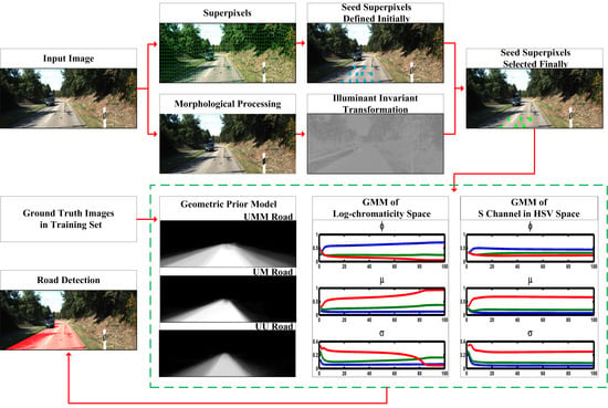
2. Proposed Algorithm

In this section, we present our proposed algorithm whose overview is illustrated in Figure 1. The algorithm consists of three major components, including the preprocessing of the input image, the estimate of the appearance model, and construction of a geometric prior model. The details of each component are discussed in the following subsections.

2.1. Preprocessing of the Input Image

2.1.1. Superpixels

Conventional road detection algorithms using monocular color images usually define features by exploiting each pixel in the input image independently. However, in this paper, we estimate the appearance model of the road surface via superpixels. Superpixels are kinds of mid-level visual cues, which have been applied to image segmentation and object detection with demonstrated success [31,32]. We choose to over-segment the images into superpixels as one of the preprocessing steps in road detection due to the following reasons: Firstly, superpixels are obtained by over-segmentation of the image into atomic regions which are ideally similar in color and texture. As a consequence, features can be well defined over a superpixel. Secondly, using each pixel independently will lead to errors in road detection resulting from various noise. On the contrary, using superpixels as elementary units can reduce the amount of noise. Thirdly, superpixels can increase the chances that the boundaries of different semantic classes are extracted. In other words, superpixels can be used to preserve boundaries, which boosts the performance of our road detection algorithm. Finally, pixel-based methods increase the complexity of inference algorithms owing to the large number of variables in high resolution images. Conversely, superpixel-based representations can reduce the computational complexity of the algorithm, because by treating each superpixel as one elementary unit, the number of total variables will be largely reduced.

In this paper, we generate superpixels as shown in Figure 1 using the SLIC (simple linear iterative clustering) method, which was proposed in [33]. In addition, for each superpixel in the input image, we compute the average feature value of all the pixels composing the corresponding superpixel.

2.1.2. Lane Markings Removal by Morphological Processing

Lane markings, which always exist on urban roads in the form of white lines, are a disadvantage for appearance based road detection algorithms. Specifically, to estimate the road model, pixels placed at the bottom part of road images are usually selected as seeds. In this case, algorithms will fail if the pixels of the lane markings are chosen to estimate the road model. It is important to mention that even though we have selected seed pixels and estimated the road model correctly, the lane markings, which actually show drivable area, will be detected as a non-road region due to their different appearance from the road surface.

To tackle this problem, we propose a novel method to remove most of the lane markings by way of morphological image processing. In this paper, the opening operation is carried out for the lane markings which have higher brightness properties than the road surface. As described in [34], opening generally breaks narrow isthmuses, smoothes contours, and eliminates thin protrusions. The opening of image $A$ by structuring element $B$, denoted $A\circ B$, is defined as follows:

$$A\circ B=(A\Theta B)\oplus B$$

(1)

where the structuring element is actually a shape in the form of a small binary matrix, used to probe or interact with a given image. Thus, the opening is the erosion of $A$ by $B$, followed by a dilation of the result by $B$. The erosion of $A$ by $B$ is denoted as $A\Theta B$, and the dilation of $A$ by $B$ is denoted as $A\oplus B$. Respectively, for the input RGB image, the value of the output pixel via erosion is the minimum value of all the pixels in the input pixel’s neighborhood, with that neighborhood defined by the structuring element; the value of the output pixel via dilation is the maximum value of all the pixels in the input pixel’s neighborhood, with that neighborhood defined by the structuring element. Note that since a characteristic of the lane markings is that the horizontal length is much smaller than the vertical length, we use a line-shaped structuring element with a length of 15 pixels at an angle of 0 degrees to carry out the opening operation. Results of the morphological processing are illustrated in Figure 1.

2.1.3. Illuminant Invariant Transformation

Color information is a powerful cue for appearance based road detection methods. However, these methods usually fail since the color of the road varies significantly depending on the acquisition conditions. Especially, shadows and highlights appearing in the road images have the greatest impact since they often lead to false road detection. To solve this problem, illuminant invariant information is needed to provide robustness to lighting conditions. In this paper, we follow the photometric invariant approach proposed in [25].

Under PLN (Planckian light source, Lambertian surfaces, and narrowband imaging sensors) assumptions, the input image is converted to an illuminant invariant space denoted by $ℐ$. For the pixel $i$ in the input image, ${ℐ}_i$ is defined as follows:

$${ℐ}_i=r_i\times \cos \theta +b_i\times \sin \theta ,$$

(2)

$$r_i=\log (R_i/G_i),$$

(3)

$$b_i=\log (B_i/G_i),$$

(4)

where $r_i$ and $b_i$ are the corresponding log-chromaticity values using the G channel for normalization, with $R_i$, $G_i$, and $B_i$ representing the stand RGB color channels of the image after morphological processing. Then, as shown in Figure 2, a set of color surfaces of a given chromaticity value imaged under different lighting conditions are projected onto a straight line in the log-chromaticity space. After that, sets of color surfaces with different chromaticity values form parallel lines. In addition, these straight lines define an orthogonal axis ${\ell }_{\theta }$, where surfaces under different illuminations are represented by the same point. Movements along ${\ell }_{\theta }$ imply changing the chromaticity value of the surface, which are independent of illumination.

Finally, following this approach, a shadow-free and highlight-free grayscale image is obtained, which is invariant under different lighting conditions. It is important to mention that converting RGB images requires knowledge of $\theta$, i.e., the illuminant invariant angle, which is an intrinsic parameter of the camera and can be calibrated by entropy-minimization. The value of the $\theta$ used in our experiments is 48.7°. Results of the illuminant invariant transformation are shown in Figure 1.

Unfortunately, lots of detail information will be decimated in the process of derivation. Alvarez et al. [35] argued that HSV color space provides diversified pixel information which can be efficiently exploited to detect road surfaces where HSV means hue, saturation and value channels in color images. Motivated by this, we use a log-chromaticity space to provide a high invariance to shadows and highlights, then we use the HSV color space to recover detail information and provide a high discriminative power. Specifically, experimental results show that the best performance is obtained when we combine the log-chromaticity space and the S (saturation) channel in the HSV color space.

2.2. Estimate of Appearance Model

2.2.1. Seed Superpixels Selection

In order to deal with the highly dynamic nature of road surfaces, current algorithms usually estimate the road model online by defining a sufficient number of seed pixels, which is based on the assumption that the bottom region of the input image belongs to road area. This assumption comes from the fact that the bottom part of the input image usually corresponds to a distance of few meters from the ego-vehicle. Nevertheless, it suffers from a major challenge: in some scenarios, the bottom part of the image may correspond to lane markings or damaged road area which cannot be representative of the road surface and thus leads to a failed estimation of the road model.

In this paper, we estimate the appearance model of road surface based on the generated superpixels. Specifically, we define 12 superpixels located at the fixed position of the input image as seeds. In view of the fact that these seeds may correspond to damaged road area and lane markings, we choose 6 of the 12 superpixels with the greatest similarity as the final seed superpixels. As shown in Equation (5), the Bhattacharyya coefficient is exploited to measure the similarity of any two superpixels, denoted as $p$ and $q$. The greater the value of $\rho$, the more similar the two superpixels.

$$\rho (p,q)={\displaystyle \sum _i\sqrt{p(i)q(i)}}.$$

(5)

Specifically, we first build the normalized histograms of the 12 superpixels using the grayscale channel of the input image. Then the similarity of any two superpixels is measured using Equation (5), where the value of i is 8, i.e., we build the normalized histogram with 8 bins. Thus we obtain a matrix of 12 × 12. Next, we sum up the 12 values of each column in the matrix. Finally, we choose the 6 superpixels whose corresponding sum is bigger than the other ones as the final seed superpixels.

The results of the seed superpixels selection are illustrated in Figure 3, where the blue superpixels show the seed superpixels defined initially and the green superpixels show the final seed superpixels selected by the Bhattacharyya coefficient.

2.2.2. Gaussian Mixture Model

In this section, we estimate the appearance model of the road surface in log-chromaticity space and the S channel in HSV color space using the Gaussian mixture model (GMM) based on the selected seed superpixels. GMM is a classical and currently widely used method. Furthermore, unlike discriminative methods, GMM delivers a probability map which allows us to fuse it with road geometric prior, which will be discussed subsequently. Here, for log-chromaticity space or the S channel in HSV color space, the value $P\left(X\right)$ which depicts the probability of the superpixel $X$ with the mean value $f_X$ in log-chromaticity space or the S channel belonging to road is defined as

$$P\left(X\right)={\displaystyle \sum _{i=1}^K{\omega }_i\times \eta \left(f_X,{\mu }_i,{\Sigma }_i\right)},$$

(6)

$$\eta \left(f_X,\mu ,\Sigma \right)=\frac{1}{{((2\pi )\times |\Sigma |)}^{\frac{1}{2}}}exp(-\frac{1}{2}{(f_X-\mu )}^T{\Sigma }^{-1}(f_X-\mu )),$$

(7)

$${\displaystyle \sum _{i=1}^K{\omega }_i}=1,$$

(8)

where $K$ gives the number of Gaussian components, ${\omega }_i$ is the weight assigned to the corresponding Gaussian component having the mean ${\mu }_i$ and covariance matrix ${\Sigma }_i$, and $\eta$ is the Gaussian probability density function defined in (7). We optimize the parameters of ${\omega }_i$, ${\mu }_i$, and ${\Sigma }_i$ with the expectation-maximization (EM) algorithm in log-chromaticity space or the S channel respectively based on the selected seed superpixels. In view of effectiveness and robustness, the value of $K$ is set to three. Thus, we obtain $P^{log}\left(X\right)$ and $P^S\left(X\right)$ which correspondingly depict the probability of the superpixel $X$ belonging to road in log-chromaticity space and the S channel in HSV color space. For the combination of color channels, we compute the average value of the color channels’ $P(X)$ as the final $P_a(X)$ which depicts the probability of the superpixel $X$ belonging to road surface according to the appearance cue. Additionally, each pixel in the superpixel $X$ shares the same value, i.e.,

$$P_a\left(x\right)=P_a\left(X\right)x=1,2,3,\cdots ,n,$$

(9)

where $n$ gives the number of pixels in the superpixel $X$. Hence, a probability map based on appearance cues denoted as $P_a$ is obtained by calculating the $P_a\left(X\right)$ of all the superpixels in the input image.

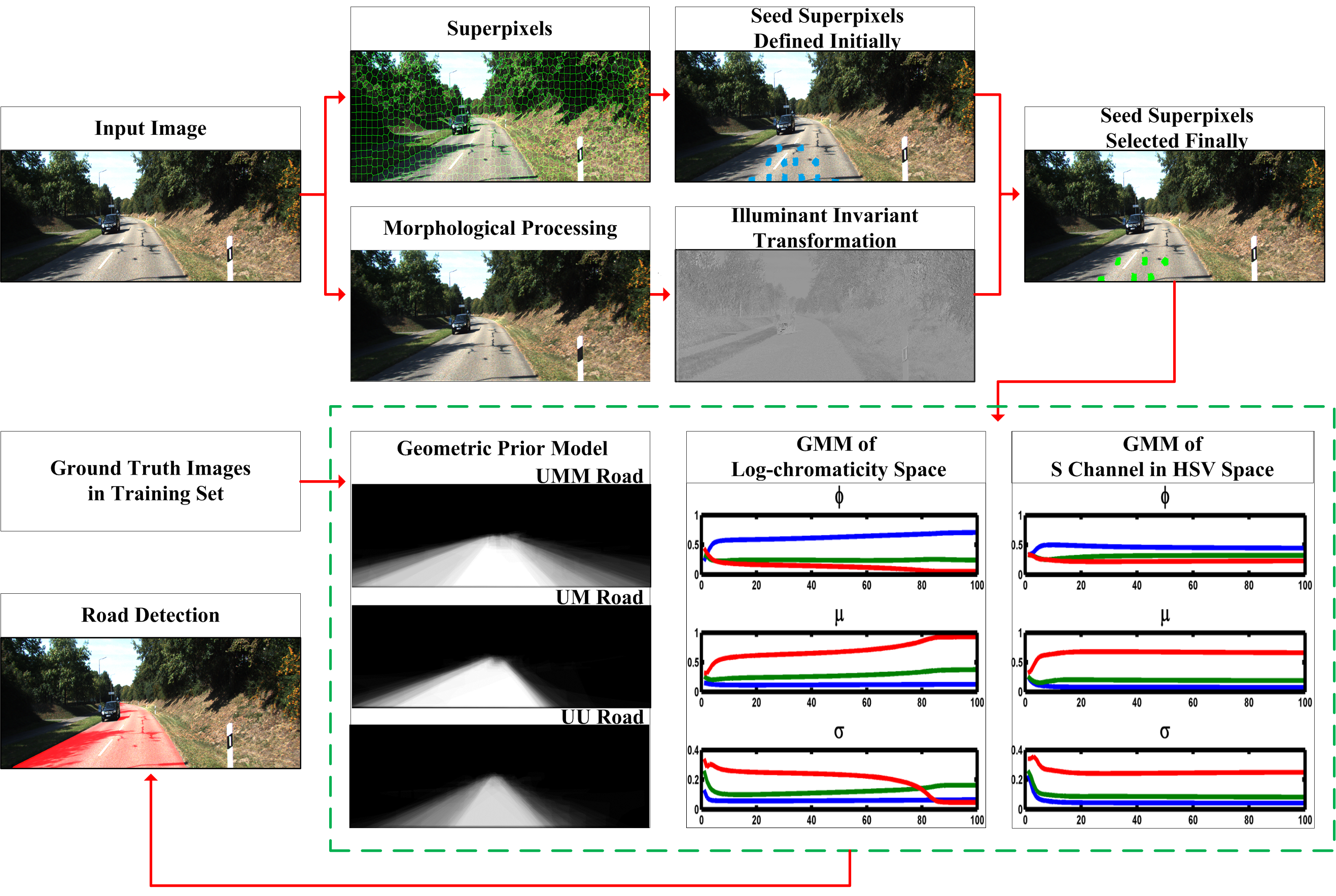
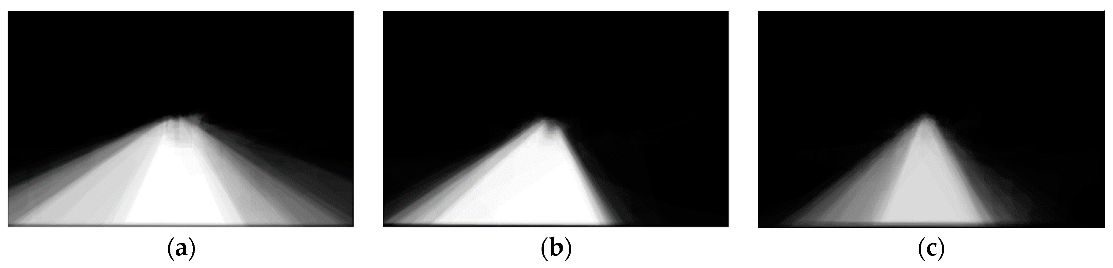
2.3. Construction of the Geometric Prior Model

Most monocular road detection algorithms usually fail to make good use of the geometric prior information which can be very helpful for reducing ambiguity and improving accuracy. As we mentioned above, road probability maps computed using appearance cues can depict the potential of a pixel being road surface. Unfortunately, it will fail when there are objects which are made of similar material and have a similar appearance to road surface in the image, for example, sidewalks, buildings, and overpasses.

In order to improve the robustness and reliability of the algorithm, we propose the novel idea to construct a geometric prior model offline. Considering that the camera mounted on the ego-vehicle is usually fixed to the windshield, as a consequence pixels of the road surface will be concentrated in a specific part of the images. In other words, nearly all the road pixels occur towards the bottom region of the image; conversely, there are never road pixels appearing at the top of the image. In view of this, by aggregating and averaging all the ground truth images provided by the KITTI road benchmark in the training set, we can obtain probability maps as illustrated in Figure 4 which indicate how frequently the road pixels occur in the corresponding position. We regard this probability map as the empirical geometric prior model $P_r$ and it will be fused with the appearance model to boost the performance of the algorithm.

2.4. Fusion of Appearance and Prior Cues

In this section, appearance and geometric prior cues are fused in a Bayesian framework to classify all the pixels of the input images as belonging or not belonging to the road surface. The final confidence map is computed as:

$$p\left(x\right)=\frac{p_r(x)p_a(x)}{p_r(x)p_a(x)+p_r’(x)p_a’(x)},$$

(10)

$$p_r’\left(x\right)=1-p_r(x),$$

(11)

$$p_a’\left(x\right)=1-p_a(x),$$

(12)

where $p_r(x)$, $p_a(x)$, and $p(x)$ show the probability of the pixel $x$ belonging to the road surface based on the geometric prior model, the appearance model, and the final confidence map, respectively. Once the confidence map is obtained, we use a classifier to assign a road or non-road label to each pixel by applying thresholds to the confidence map according to the following rule:

$$p(x)=\{\begin{array}{ll}road& if:p(x)>\lambda \\ nonroad& otherwise\end{array}.$$

(13)

We conduct experiments to select the optimal value of the threshold $\lambda$, which will be given in Section 3.2.2.

3. Experimental Results and Discussion

In this section, experiments have been conducted to evaluate the performance of the proposed method. Firstly, we introduce the dataset and platform of our experiment. Then, a detailed description of experimental results is reported, including the evaluation of variant combinations of color channels, the optimization of the threshold, the qualitative evaluation, and the quantitative evaluation. Finally, a discussion based on the experimental results is given.

3.1. Dataset and Platform of the Experiment

The KITTI (Karlsruhe Institute of Technology and Toyota Technological Institute) road benchmark [36] has 289 images in the training set with their ground-truth provided and 290 images in the testing set. All of these images were taken on the streets of Karlsruhe, Germany with the resolution of 1242 × 375 pixels. Images in the dataset show a variety of road situations and are divided into three categories, namely urban multiple marked (UMM), urban marked (UM), and urban unmarked (UU).

All the following experiments are tested on a personal laptop computer with 8 GB of RAM and an Intel Core i7-6700 CPU@ 2.5 GHz. The computation environment is MATLAB R2017b.

3.2. Experimental Results

3.2.1. Evaluation of Variant Combinations of Color Channels

As described in Section 2.1.3, shadow-free and highlight-free grayscale images are obtained by illuminant invariant transformation. To recover detail information and provide higher discriminative power, HSV color space is combined with the log-chromaticity space.

In order to evaluate the performance of variant combinations of color channels, we use receiver operating characteristic (ROC) curves on the comparison between the results of road detection and ground-truth provided in the KITTI road benchmark training set. ROC curves show the trade-off between the true positive rate (TPR) and the false positive rate (FPR) at various threshold λ settings, which are defined as follows:

$$TPR=\frac{TP}{TP+FN},$$

(14)

$$FPR=\frac{FP}{FP+TN},$$

(15)

where TP means true positive, FN means false negative, FP means false positive, and TN means true negative. In addition, we use the area under the curve (AUC) for performance comparisons. The higher the value of the AUC, the higher the accuracy. Results are shown in Figure 5.

As shown, higher performance is achieved when H, S, and V channels are combined with the log-chromaticity space. However, the worst performance appears when all of the log-chromaticity and H, S, and V channels are used simultaneously since the robustness to shadows and highlights of the log-chromaticity space is badly weakened by the entire HSV color space. From these results, we can conclude that the highest performance is provided by combining the log-chromaticity space and the S channel in HSV color space.

3.2.2. Optimization of the Threshold

To optimize the threshold, we sweep over a sufficient range of thresholds based on the confidence map and compute the average intersection-over-union (IOU) of the detected road surface with the ground-truth provided in the training set. As shown in Figure 6, the optimal value of the threshold that maximizes the IOU is 0.81, which is selected in our experiments to divide the confidence map into road and non-road regions.

3.2.3. Qualitative Evaluation

Considering that our method is model-based and the appearance model is built online, we test it on both the training set and testing set. Figure 7 shows sample road detection results of some images from the training set captured in challenging scenarios, including different backgrounds, varying illumination, variability of road appearance, and differently shaped objects. To better show the effectiveness of the proposed algorithm, we present the comparison among ground-truths provided in the training set, our road detection results without prior cues, and results fusing appearance and prior cues.

Figure 8 shows some sample road detection results from the testing set. Additionally, some other recently developed state-of-the-art methods which show excellent performance and rank high on the KITTI road benchmark are used for the purpose of comparison. These algorithms include SRF [6], CN [7], FCN–LC [12], BM [24], ANN [27] and LidarHisto [29].

3.2.4. Quantitative Evaluation

In this section, quantitative evaluations of our proposed algorithm for images in the testing set are provided using five classical metrics known as precision (PRE), recall (REC), maximum F1-measure (MaxF), false positive rate (FPR), and false negative rate (FNR). Where the metric PRE measures what percentage of the road detection results are truly road, the metric REC reflects how much of the overall road region was detected, the metric MaxF gives a tradeoff between PRE and REC, the metric FPR measures how much of the non-road region was improperly detected as road region, and the metric FNR measures how much of the road region was improperly detected as non-road region. The metrics are calculated as follows:

$$PRE=\frac{TP}{TP+FP},$$

(16)

$$REC=\frac{TP}{TP+FN},$$

(17)

$$F1-measure=\frac{PRE\times REC}{(1-\alpha )\times PRE+\alpha \times REC},where\alpha =0.5,$$

(18)

$$FPR=\frac{FP}{FP+TN},$$

(19)

$$FNR=\frac{FN}{TP+FN}.$$

(20)

Note that the metrics are computed after the transformation from an image domain to bird’s-eye-view (BEV) space according to the evaluation system of the KITTI road benchmark.

Results of the quantitative evaluation of the proposed algorithm are reported together with the results of the other state-of-the-art algorithms mentioned in Section 3.2.3. Specifically, the comparison of UMM_ROAD, UM_ROAD, and UU_ROAD is shown in

Table 1. Evaluation of UMM_ROAD (bird’s-eye-view (BEV)).

Method	PRE (%)	REC (%)	MaxF (%)	FPR (%)	FNR (%)
SRF [6]	89.35	92.23	90.77	12.08	7.77
CN [7]	82.85	89.86	86.21	20.45	10.14
FCN–LC [12]	94.05	94.13	94.09	6.55	5.87
BM [24]	83.43	96.30	89.41	21.02	3.70
ANN [27]	69.95	96.05	80.95	45.35	3.95
LidarHisto [29]	95.39	91.34	93.32	4.85	8.66
Our method	93.46	95.33	94.39	1.76	4.67

,

Table 2. Evaluation if UM_ROAD (BEV).

Method	PRE (%)	REC (%)	MaxF (%)	FPR (%)	FNR (%)
SRF [6]	75.53	77.35	76.43	11.42	22.65
CN [7]	69.18	78.83	73.69	16.00	21.17
FCN–LC [12]	89.35	89.37	89.36	4.85	10.63
BM [24]	69.53	91.19	78.90	18.21	8.81
ANN [27]	50.21	83.91	62.83	37.91	16.09
LidarHisto [29]	91.28	88.49	89.87	3.85	11.51
Our method	89.93	93.46	91.66	2.79	6.54

, and

Table 3. Evaluation of UU_ROAD (BEV).

Method	PRE (%)	REC (%)	MaxF (%)	FPR (%)	FNR (%)
SRF [6]	71.47	81.31	76.07	10.57	18.69
CN [7]	71.96	72.54	72.25	9.21	27.46
FCN–LC [12]	86.65	85.89	86.27	4.31	14.11
BM [24]	70.87	87.80	78.43	11.76	12.20
ANN [27]	39.28	86.69	54.07	43.67	13.31
LidarHisto [29]	90.71	82.75	86.55	2.76	17.25
Our method	91.66	89.93	90.79	2.55	10.07

respectively. In addition, a category named URBAN_ROAD which provides the overall performance for all three categories is calculated and the comparison result is shown in

Table 4. Evaluation of URBAN _ROAD (BEV).

Method	PRE (%)	REC (%)	MaxF (%)	FPR (%)	FNR (%)
SRF [6]	80.60	84.36	82.44	11.18	15.64
CN [7]	76.64	81.55	79.02	13.69	18.45
FCN–LC [12]	90.87	90.72	90.79	5.02	9.28
BM [24]	75.90	92.72	83.47	16.22	7.28
ANN [27]	54.19	90.17	67.70	41.98	9.83
LidarHisto [29]	93.06	88.41	90.67	3.63	11.59
Our method	92.04	92.98	92.51	2.46	7.02

.

3.3. Discussion

From these experimental results, we can conclude that our proposed method provides remarkable road detection results when we select the optimal value of the threshold and combine the log-chromaticity space with the S channel in HSV color space to estimate the appearance model. Moreover, qualitative and quantitative evaluations on the KITTI road benchmark demonstrate that appearance cues are essential to obtain reliable road detection results and geometric prior cues provide relevant information to infer the location of the road surface, thus higher performance is obtained when fusing appearance and prior cues.

It is important to mention that we obtained geometric prior models of UMM, UM, and UU road in view of the fact that images in the KITTI road benchmark are divided into three corresponding categories. Consequently, for each input image in a certain category, we use the corresponding geometric prior model. On the contrary, the other competing state-of-the-art methods mentioned above use a single algorithm for all three categories of images in the KITTI road benchmark. We have conducted experiments and the results show that for all the images in the dataset, a decrease of less than 0.3% of the MaxF score, i.e., almost the same performance of road detection, can be achieved when we use the non-corresponding geometric prior model. We argue that this happens since appearance cues are essential in our algorithm and prior cues provide statistical descriptions and information which are in principle similar along with the variety of road situations. Actually, we can aggregate and average all the ground-truth images, no matter which category, to obtain a single geometric prior model in practical application.

Finally, we conduct an analysis of the computational cost of the proposed method. We run our experiments with non-optimized MATLAB code. The entire road detection process takes about 1800 ms on images with the resolution of 1242 × 375 pixels. We think that it is possible to run in less than 300 ms with C++ code. In addition, there are some optimizations, such as using gSLICr [37] which is a GPU-implementation of the SLIC algorithm. Furthermore, considering that one third of the upper part of the input images are not likely to contain any road area, and we can remove it as [25] suggested. In contrast to our proposed algorithm, the computational cost of the other state-of-the-art methods mentioned above are as follows: SRF [6] takes about 0.2 s with C++ code using a CPU @ 2.5 GHz; CN [7] takes about 2 s with C++ code using a CPU @ 2.5 GHz; FCN–LC [12] takes about 0.03 s with Python code using an additional GPU Titan X; BM [24] takes about 2 s with MATLAB code using 2 CPU @ 2.5 GHz; ANN [27] takes about 3 s with C++ code using a CPU @ 3.0 GHz; LidarHisto [29] takes about 0.1 s with C++ code using a CPU @ 2.5 GHz.

4. Conclusions and Future Work

In this paper, we have developed a novel method of fusing appearance and prior cues for road detection. Firstly, in view of the fact that the pixels of lane markings are usually selected as seeds and classified as non-road regions in previous appearance based algorithms, we propose a novel method to remove lane markings by way of morphological image processing. Further, to improve robustness to lighting conditions, we obtain illuminant invariant information using log-chromaticity space. We also use the S channel in HSV color space to recover detail information decimated in log-chromaticity space. Then, we estimate the road appearance model online via superpixels and design a novel seed superpixels selection method to adapt the highly dynamic nature of road surfaces. Finally, we construct a road geometric prior model offline and fuse appearance and prior cues with a Bayesian framework to improve the performance of the algorithm.

Experiments have been conducted on the KITTI road benchmark and it can be concluded that using prior cues results in a noticeable improvement since geometric prior information provides statistical descriptions and relevant information to infer the location of the road surface. Moreover, the proposed method of fusing appearance and prior cues can provide reliable road detection results and show robustness to various driving scenarios. In addition, the proposed algorithm achieves state-of-the-art performance with a MaxF score of 92.51% in the urban category among the model-based methods. Generally, both the robustness and accuracy can be satisfied in various driving scenarios which is necessary for practical use in autonomous driving system and driver assistance system. In future research, we intend to accelerate the processing speed of the algorithm and make it more efficient to meet real-time demand.

References

1. Hillel, A.B.; Lerner, R.; Dan, L.; Raz, G. Recent progress in road and lane detection: a survey. Mach. Vis. Appl. 2014, 25, 727–745. [Google Scholar] [CrossRef]
2. Janai, J.; Güney, F.; Behl, A.; Geiger, A. Computer Vision for Autonomous Vehicles: Problems, Datasets and State-of-the-Art. arXiv, 2017; arXiv:1704.05519. [Google Scholar]
3. Yasrab, R.; Gu, N.; Zhang, X. An Encoder-Decoder Based Convolution Neural Network (CNN) for Future Advanced Driver Assistance System (ADAS). Appl. Sci. 2017, 7, 312. [Google Scholar] [CrossRef]
4. Chacra, D.A.; Zelek, J. Road Segmentation in Street View Images Using Texture Information. In Proceedings of the Computer & Robot Vision, Victoria, BC, Canada, 1–3 June 2016. [Google Scholar]
5. Zhou, S.; Gong, J.; Xiong, G.; Chen, H.; Iagnemma, K. Road detection using support vector machine based on online learning and evaluation. In Proceedings of the Intelligent Vehicles Symposium, San Diego, CA, USA, 21–24 June 2010. [Google Scholar]
6. Xiao, L.; Dai, B.; Liu, D.; Zhao, D.; Wu, T. Monocular road detection using structured random forest. Int. J. Adv. Robot. Syst. 2016, 13, 101. [Google Scholar] [CrossRef]
7. Alvarez, J.M.; Gevers, T.; Lecun, Y.; Lopez, A.M. Road Scene Segmentation from a Single Image. Proc. Eur. Conf. Comput. Vis. 2012. [Google Scholar] [CrossRef]
8. Long, J.; Shelhamer, E.; Darrell, T. Fully convolutional networks for semantic segmentation. IEEE Trans. Pattern Anal. Mach. Intell. 2014, 39, 640–651. [Google Scholar]
9. Gao, J.; Qi, W.; Yuan, Y. Embedding structured contour and location prior in siamesed fully convolutional networks for road detection. Proc. IEEE Int. Conf. Robot. Autom. 2018, 19, 230–241. [Google Scholar]
10. Zhe, C.; Chen, Z. RBNet: A Deep Neural Network for Unified Road and Road Boundary Detection. Proc. Int. Conf. Neural Inf. Process. 2017. [Google Scholar] [CrossRef]
11. Oliveira, G.L.; Burgard, W.; Brox, T. Efficient deep models for monocular road segmentation. In Proceedings of the 2016 IEEE/RSJ International Conference on Intelligent Robots and Systems (IROS), Daejeon, Korea, 9–14 October 2016; pp. 4885–4891. [Google Scholar]
12. Mendes, C.C.T.; Frémont, V.; Wolf, D.F. Exploiting fully convolutional neural networks for fast road detection. In Proceedings of the 2016 IEEE International Conference on Robotics and Automation (ICRA), Stockholm, Sweden, 16–20 May 2016; pp. 3174–3179. [Google Scholar]
13. Teichmann, M.; Weber, M.; Zoellner, M.; Cipolla, R.; Urtasun, R. MultiNet: Real-time Joint Semantic Reasoning for Autonomous Driving. In Proceedings of the 2018 IEEE Intelligent Vehicles Symposium (IV), Changshu, China, 26–30 June 2018. [Google Scholar]
14. Zeiler, M.D.; Fergus, R. Visualizing and Understanding Convolutional Networks; Springer: Cham, Switzerland, 2013. [Google Scholar]
15. Kong, H.; Audibert, J.Y.; Ponce, J. Vanishing point detection for road detection. Comput. Vis. Pattern Recog. 2013, 2009, 96–103. [Google Scholar]
16. Hui, K.; Jean-Yves, A.; Jean, P. General road detection from a single image. IEEE Trans. Image Process. A Publ. IEEE Signal Process. Soc. 2010, 19, 2211–2220. [Google Scholar]
17. Helala, M.A.; Pu, K.Q.; Qureshi, F.Z. Road Boundary Detection in Challenging Scenarios. In Proceedings of the IEEE Ninth International Conference on Advanced Video & Signal-based Surveillance, Taipei, Taiwan, 18–21 September 2019. [Google Scholar]
18. Nan, Z.; Wei, P.; Xu, L.; Zheng, N. Efficient Lane Boundary Detection with Spatial-Temporal Knowledge Filtering. Sensors 2016, 16, 1276. [Google Scholar] [CrossRef] [PubMed]
19. Geng, Z.; Zheng, N.; Chao, C.; Yan, Y.; Yuan, Z. An efficient road detection method in noisy urban environment. In Proceedings of the Intelligent Vehicles Symposium, Xi’an, China, 3–5 June 2009. [Google Scholar]
20. Broggi, A.; Bertè, S. Vision-Based Road Detection in Automotive Systems: A Real-Time Expectation-Driven Approach. J. Artif. Intell. Res. 1995, 3, 325–348. [Google Scholar] [CrossRef]
21. He, Y.; Wang, H.; Zhang, B. Color-based road detection in urban traffic scenes. IEEE Trans. Intell. Transp. Syst. 2004, 5, 309–318. [Google Scholar] [CrossRef]
22. Tan, C.; Hong, T.; Chang, T.; Shneier, M. Color model-based real-time learning for road following. In Proceedings of the IEEE Intelligent Transportation Systems Conference, Toronto, ON, Canada, 17–20 September 2006. [Google Scholar]
23. Zhang, H.; Hernandez, D.; Su, Z.; Su, B. A Low Cost Vision-Based Road-Following System for Mobile Robots. Appl. Sci. 2018, 8, 1635. [Google Scholar] [CrossRef]
24. Wang, B.; Fremont, V.; Rodriguez, S.A. Color-based road detection and its evaluation on the KITTI road benchmark. In Proceedings of the Intelligent Vehicles Symposium, Dearborn, MI, USA, 3–5 October 2000. [Google Scholar]
25. Alvarez, J.M.Á.; Lopez, A.M. Road Detection Based on Illuminant Invariance. IEEE Trans. Intell. Transp. Syst. 2011, 12, 184–193. [Google Scholar] [CrossRef]
26. Scharwachter, T.; Franke, U. Low-level fusion of color, texture and depth for robust road scene understanding. In Proceedings of the Intelligent Vehicles Symposium, Seoul, Korea, 29 June–1 July 2015. [Google Scholar]
27. Vitor, G.B.; Lima, D.A.; Victorino, A.C.; Ferreira, J.V. A 2D/3D Vision Based Approach Applied to Road Detection in Urban Environments. In Proceedings of the Intelligent Vehicles Symposium, Gold Coast, Australia, 23–26 June 2013. [Google Scholar]
28. Caltagirone, L.; Bellone, M.; Svensson, L.; Wahde, M. LIDAR-Camera Fusion for Road Detection Using Fully Convolutional Neural Networks. Robot. Auton. Syst. 2018, 111, 125–131. [Google Scholar] [CrossRef]
29. Liang, C.; Jian, Y.; Hui, K. Lidar-histogram for fast road and obstacle detection. In Proceedings of the IEEE International Conference on Robotics & Automation, Singapore, 29 May–3 June 2017. [Google Scholar]
30. Laddha, A.; Kocamaz, M.K.; Navarro-Serment, L.E.; Hebert, M. Map-supervised road detection. In Proceedings of the Intelligent Vehicles Symposium, Gothenburg, Sweden, 19–22 June 2016. [Google Scholar]
31. Zhao, W.; Zhang, H.; Yan, Y.; Fu, Y.; Wang, H. A Semantic Segmentation Algorithm Using FCN with Combination of BSLIC. Appl. Sci. 2018, 8, 500. [Google Scholar] [CrossRef]
32. Zhao, W.; Fu, Y.; Wei, X.; Wang, H. An Improved Image Semantic Segmentation Method Based on Superpixels and Conditional Random Fields. Appl. Sci. 2018, 8, 837. [Google Scholar] [CrossRef]
33. Achanta, R.; Shaji, A.; Smith, K.; Lucchi, A.; Fua, P.; Süsstrunk, S. SLIC Superpixels Compared to State-of-the-Art Superpixel Methods. IEEE Trans. Pattern Anal. Mach. Intell. 2012, 34, 2274–2282. [Google Scholar] [CrossRef] [PubMed] [Green Version]
34. Gonzalez, R.C.; Wintz, P. Digital Image Processing; Addison-Wesley Longman Publishing Co., Inc.: Boston, MA, USA, 2007. [Google Scholar]
35. Alvarez, J.M.; Gevers, T.; Lopez, A.M. Evaluating Color Representations for On-Line Road Detection. In Proceedings of the IEEE International Conference on Computer Vision Workshops, Sydney, Australia, 1–8 December 2013. [Google Scholar]
36. Fritsch, J.; Kuhnl, T.; Geiger, A. A new performance measure and evaluation benchmark for road detection algorithms. In Proceedings of the International IEEE Conference on Intelligent Transportation Systems, The Hague, The Netherlands, 6–9 October 2013. [Google Scholar]
37. Ren, C.Y.; Prisacariu, V.A.; Reid, I.D. gSLICr: SLIC superpixels at over 250 Hz. arXiv, 2015; arXiv:1509.04232. [Google Scholar]
Figure 1. Overview of our proposed algorithm for road detection.
Applsci 09 00996 g001
Figure 2. Illuminant invariant transformation.
Applsci 09 00996 g002
Figure 3. Seed superpixels selection. (a) Seed superpixels defined initially; (b) final seed superpixels selected.
Applsci 09 00996 g003
Figure 4. The geometric prior model. (a) Urban multiple marked (UMM) road; (b) Urban marked (UM) road; (c) Urban unmarked (UU) road. The whiter the color, the higher the probability to be road surface.
Applsci 09 00996 g004
Figure 5. Receiver operating characteristic (ROC) curves based on variant combinations of color channels. The ‘log’ represents the log-chromaticity space, and ‘H’, ‘S’, and ‘V’ represent hue, saturation, and value channels in HSV color space.
Applsci 09 00996 g005
Figure 6. Optimization of the threshold.
Applsci 09 00996 g006
Figure 7. Sample visual comparison on the Karlsruhe Institute of Technology and Toyota Technological Institute (KITTI) training set. First row: input images; second row: road detection results without prior cues; third row: detected road surfaces without prior cues; fourth row: road detection results fusing appearance and prior cues; fifth row: detected road surfaces fusing appearance and prior cues; sixth row: corresponding ground-truths.
Applsci 09 00996 g007
Figure 8. Sample visual comparison on the KITTI testing set.
Applsci 09 00996 g008