A Multi-Period Approach for the Optimal Energy Retrofit Planning of Street Lighting Systems

Abstract

Investing in the optimal measures for improving the energy efficiency of urban street lighting systems has become strategic for the economic, technological and social development of cities. The decision-making process for the selection of the optimal set of interventions is not so straightforward. Several criticalities-such as difficulties getting access to credit for companies involved in street lighting systems refurbishment, budget constraints of municipalities, and unawareness of the actual energy and economic performance after a retrofitting intervention-require a decision-making approach that supports the city energy manager in selecting the optimal street lighting energy efficiency retrofitting solution while looking not only based on the available budget, but also based on the future savings in energy expenditures. In this context, the purpose of our research is to develop an effective decision-making model supporting the optimal multi-period planning of the street lighting energy efficiency retrofitting, which proves to be more effective and beneficial than the classical single-period approach and has never before been applied to the considered public lighting system context. The proposed methodology is applied to a real street lighting system in the city of Bari, Italy, showing the energy savings and financial benefit obtained through the proposed method. Numerical experiments are used to investigate and quantify the effects of using a multi-period planning approach instead of a single-period approach.

1. Introduction

Energy consumption for urban street lighting has assumed considerable importance in the energy and economic balance for many cities [1,2]. Public lighting systems are a major source of electricity consumption: at present 3.19% of global electricity generation is used for lighting. This amount is greater than production of all hydro or nuclear plants and equals the production from natural gas [3]. It is widely recognized that public lighting is a sector characterized by excessive and disproportionate energy consumption compared to the quality and functionality of the service offered to the citizen. This implies the need for tools to improve the energy performance of urban street lighting, such as new technologies, professionalism and analytical/design skills [4].

A study carried out by ENEA (the Italian National Agency for New Technologies, Energy and Sustainable Economic Development) reports that the “energy wastage” of urban street lighting systems in Italy currently accounts 30% of consumption on average [4]. This highlights the role and potential of energy efficiency processes of street lighting systems, not only in terms of environmental performance (due to reduction of energy consumption and emissions of CO₂ into the atmosphere), but also in terms of economic and financial performance (due to the reduction of economic costs of bills, which today heavily burden municipal budgets).

The strategic role of the public lighting sector as a drive for the economic, technological and social development of cities justifies the increasing commitment of city authorities to energy efficiency and green energy public lighting systems. The European Community provides several policy tools in order to achieve these savings. One of the most important is the “Covenant of Majors” (4400 partners of which 2100 are Italian Municipalities) which groups local and regional European authorities, with these groups voluntarily committing to improving energy efficiency and the use of renewable energy sources on their territories [5].

The increasing attention reserved by practitioners and city authorities to the topic has been accompanied by the development of much research in the field. Most of the existing studies aim at developing optimization models for selecting the right energy efficiency measures among a set of alternatives, by looking at the whole street lighting system or even parts of it. Popa and Cepişcă [6] propose a consumption reducing solution based on an intelligent system for remote sensing and control with dimming technologies of HID (high-intensity discharge) lamps. Raciti et al. [7] develop a tool for an optimal lighting system design aiming at reducing both costs and distortion of the whole lighting system. Beccali et al. [1] investigate the effect of three strategies on the performance of street lighting systems: the first consists of adopting lighting controllers on each switchboard, the second of changing the existing lamps with LED (light-emitting diode) luminaires, and the third involves combining both of the previous strategies. Carli et al. [8] develop a multi-criteria decision-making tool to support the public decision maker in optimizing energy retrofit interventions on existing public street lighting systems. Cristea et al. [9] propose a multi-criteria decision-making approach for selecting optimal technical and economic solution for public lighting system. Beccali et al. [10] propose a multi-objective methodology (including lighting, energy and economic parameters) for street lighting systems refurbishment evaluation in small/medium sized Italian towns.

By looking at the decision-making process for the selection of the set of interventions to improve the energy efficiency of a street lighting system, it is possible to highlight some criticalities, such as: difficulties in gaining access to credit by companies involved in the refurbishment of lighting systems in cities [11,12], budget constraints of municipalities [13], and unawareness about the actual energy and economic performance (e.g., reduction of energy consumption, savings, etc.) reached after the retrofitting intervention [14]. All these aspects favor the adoption of a multi-period planning approach, i.e., a decision-making approach that selects the optimal street lighting energy efficiency retrofitting solution looking not only at the available budget, but also at the future savings in energy expenditures that could be used to accumulate cash to invest in other technologies or subsequent interventions on the system. While multi-period planning approaches have been studied in different contexts, such as public buildings [15,16], water distribution networks [17], waste management [18], and technology projects [19], to the best of the authors’ knowledge, the related literature lacks studies focusing on this approach in the public street lighting system, which obviously has its own peculiarities compared to other sectors [8]. The purpose of our research is therefore to develop an effective decision-making model supporting the optimal multi-period planning of the street lighting energy efficiency retrofitting. The main contribution of the paper is therefore a methodology that does not optimize “one-off” interventions on the public street lighting system, but rather defines a plan of retrofitting interventions which exploits the initial budget available for the investment as well as the financial or environmental benefits and savings obtained after the implementation of energy efficiency measures. The application of the proposed methodology to a real street lighting system in the city of Bari, Italy, shows the energy and financial savings obtained by using a multi-period planning approach instead of a single-period approach. The results demonstrate the importance not only of improving the energy system performance with one-off interventions on the lighting system, but also of the continuous improvement of the system for ensuring its sustainability.

2. The Proposed Methodology

This section states the optimization problem aimed at determining the optimal multi-period energy retrofit planning for an existing street lighting system. The problem formulation is preceded by the modeling of the street lighting system and is framed into the description of the entire decision making procedure that is performed by the street lighting manager.

2.1. System Model and Decision Design

An urban street lighting system is typically widespread, with a huge number of lighting points and an extensive power and communication and control network. Consequently, it is generally composed of a set of subsystems, which reproduce the lighting conditions in the street/road segments pertaining to adjacent urban zones. All the lighting units related to a given subsystem are supplied by a power substation and are automatically regulated by a control unit.

The actual decision making is preceded by a decision design preparatory phase that comprises the analysis of the street lighting current conditions as well as the definition and characterization of appropriate retrofitting interventions, in the compliance with the norms and standards. This phase is performed by the decision maker in conjunction with technical experts on a zone by zone basis.

First, the total energy savings achieved implementing the candidate refurbishment interventions plan is identified as the optimization criterion, since commonly used for assessing the energy performance of road lighting [20]. Subsequently, an on-site audit activity is performed. For each zone lighting subsystem, a diagnosis activity is conducted to evaluate the characteristics of interest, i.e., the classification and enumerations of deployed lighting units, and their parameters. The completion of the diagnosis phase allows estimating of the ex-ante status of the whole street lighting system.

Successively, the assessment of appropriate refurbishment interventions is conducted. This activity implies an individual feasibility analysis in all the zone lighting subsystems, since each generally shows unique features, thus requiring customized retrofit measures. The outcome of such an activity is the set of possible interventions to be implemented in the given existing street lighting system, denoted as $J=\left\{1,\dots ,j,\dots ,J\right\}$. We assume that the street lighting system satisfies the minimal technical requirements (e.g., photometric features) and all the retrofit measures to be implemented do not hinder the attainment of these technical requirements, while improving energy savings. Subsequently, each retrofit measure is characterized by three parameters: the application potential, the cost, and its payoff.

The application potential of an intervention is defined as the metric concerning the maximum extension of the intervention implementation. For instance, in case of replacement of lighting units, the application potential consists in the number of units to be replaced, measured in pieces. Denoting the application potential of the $j$th action as $u_j$, we collect the application potentials of all the actions $j=1,\dots ,J$ in a column vector $\mathit{u}=\left(u_1,\dots ,u_j,\dots ,u_J\right)$.

The cost of each intervention is modeled in accordance with a linear pricing model. Therefore, denoting as $c_j$ the current unitary cost of the $j$th action, we collect all the unitary costs in a column vector $\mathit{c}=\left(c_1,\dots ,c_j,\dots ,c_J\right)$.

The payoff of the generic intervention is defined as the per-period energy saving that the application of the specific action is expected to produce on the street lighting system. The payoff of each action is also modeled in accordance with a linear model. Therefore, denoting as $p_j$ the payoff of the $j$th action, we collect all the current unitary payoffs in a column vector $\mathit{p}=\left(p_1,\dots ,p_j,\dots ,p_J\right)$. For instance, in case of the replacement of the aforementioned lighting units, the yearly energy consumption reduction per replaced lighting unit (measured in kWh/year) is assessed as $p_j=\gamma -{\gamma }^{\prime }$, where $\gamma$ and ${\gamma }^{\prime }$, are the nominal energy consumptions of lighting units of a given type before and after the luminaire replacement, respectively.

2.2. Optimization Problem Formulation

We consider both the single- and the multi-period optimization settings. In the single-period case, the energy manager aims at determining the optimal set of energy retrofit actions to be implemented all at once in the current period (“one-off” interventions)-denoted as $k=1$ —to maximize the energy saving for a given initial investment. In the multi-period case, the implementation of retrofitting interventions is spread over time and leverages the financial refunding that results from recurrent energy cost savings resulting from the preceding periods. Consequently, the energy manager aims at identifying the optimal energy retrofit actions to be implemented over all the periods-denoted as ordered sequence $\mathcal{K}=\left(1,\dots ,k,\dots ,K\right)$-to maximize the total energy saving for a given initial investment.

2.2.1. Retrofit Planning in a Single-Period Setting

The single-period decision model relies on several decision variables, reflecting the choices on the retrofitting interventions to be implemented in the existing street lighting system at the beginning of the current period $k=1$. Let ${\mathit{x}}_1=\left(x_{11},\dots ,x_{1j},\dots ,x_{1J}\right)$ denote the column vector of integer decision variables, reflecting the quantitative choices on retrofit actions implementation. For instance, if action $j$ denotes the deployment of energy harvesting modules, $x_{1j}$ represents the quantity of modules to be deployed in the given street lighting system at the beginning of the current period $k=1$. All the variables are lower bounded by zero (i.e., no intervention) and are upper bounded by the application potential of the given intervention. Indicating by ${\mathbf{0}}_J$ the $J$-dimensional zero column vector, we introduce set $\chi$ to compactly define the decision space:

$$\chi =\left\{{\mathit{x}}_1\in {\mathbb{N}}^J,\hspace{1em}\hspace{1em}{\mathbf{0}}_J\le {\mathit{x}}_1\le \mathit{u}\right\}.$$

(1)

Furthermore, the choice of the decision variables is constrained by the financial resources limitation. Assuming that different actions produce additive effects on cost and calling $b$ the budget allocated to the retrofit actions plan of the whole system at the beginning of the planning phase, the following inequality must be satisfied:

$${{\displaystyle \sum }}_{j=1}^J{c}_j{x}_{1j}={\mathit{c}}^T{\mathit{x}}_1\le b.$$

(2)

In addition, the objective function, to be maximized, is the total energy saving achieved at the end of the current period. Assuming that different actions produce additive effects on payoff, the objective function is defined by summing the payoffs resulting from implementing all the planned actions in the given street lighting system:

$$f_1\left({\mathit{x}}_1\right)={{\displaystyle \sum }}_{j=1}^J{p}_j{x}_{1j}={\mathit{p}}^T{\mathit{x}}_1.$$

(3)

Summing up, the optimization problem aimed at selecting the optimal energy retrofit of an existing street lighting system turns into determining the $J$ integer decision variables in ${\mathit{x}}_1$ to maximize the linear objective function in (3) and satisfy the $2J$ bounding constraints (1) and the inequality constraint (2):

$$\begin{gathered} \underset{{\mathit{x}}_1\in \chi }{\max }{\mathit{p}}^T{\mathit{x}}_1 \\ \mathrm{s}.\mathrm{t}.{\mathit{c}}^T\mathit{x}\le b. \end{gathered}$$

(4)

Problem (4) is a linear integer programming problem, also known as integer mono-constrained Knapsack problem [21]. A nontrivial solution of (4) can be determined by exact methods (e.g., the branch and bound method) or heuristic approaches (e.g., greedy algorithms) [21].

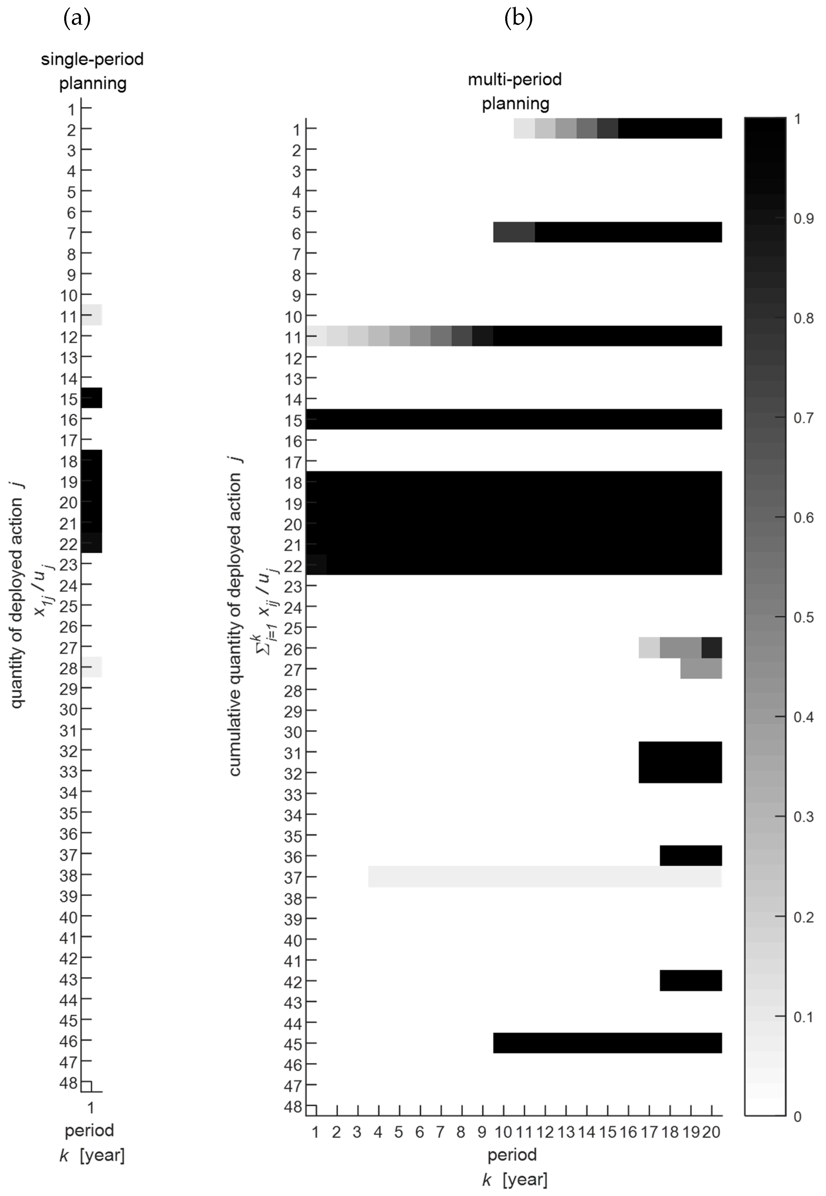
2.2.2. Retrofit Planning in a Multi-Period Setting

The multi-period decision model aims at identifying the optimal retrofitting interventions to be separately implemented at the beginning of the $K$ time periods. To this aim, $K$ column vectors of non-negative integer decision variables ${\mathit{x}}_k=\left(x_{k1},\dots ,x_{kj},\dots ,x_{kJ}\right)$ ($k=1,\dots ,K$) are defined to reflect the quantitative choices on the retrofitting interventions implementation over the given planning horizon. For instance, if action $j$ denotes the deployment of energy harvesting modules, $x_{kj}$ represents the quantity of modules to be deployed at the beginning of time interval $k$. All the decision variables are lower bounded by zero (i.e., no intervention) and are upper bounded by the application potential of the given intervention:

$${\mathit{x}}_k\in \chi ,\hspace{1em}\hspace{1em}k=1,\dots ,K.$$

(5)

In addition, $K$ column vectors of supporting integer variables $z_k=\left(z_{k1},\dots ,z_{kj},\dots ,z_{kJ}\right)$ ($k=1,\dots ,K$) are introduced to define the cumulative quantities of retrofitting interventions implemented along the time horizon. For instance, $z_{kj}$ represents the quantity of action $j$ deployed up to the time interval $k$:

$$z_{kj}={{\displaystyle \sum }}_{i=1}^k{x}_{ij},k=1,\dots ,K,j=1,\dots ,J.$$

(6)

It is apparent that also the above defined supporting variables are lower bounded by zero (i.e., no intervention) and are upper bounded by the application potential of the given interventions:

$${\mathit{z}}_k\in \chi ,\hspace{1em}\hspace{1em}k=1,\dots ,K.$$

(7)

Furthermore, differently from the single-period setting, the multi-period planning implies considering time-varying pattern for energy savings and retrofit action costs [22]. As for energy savings, we assume that the performance of the energy efficiency retrofits can deteriorate subject to usage of the retrofitted items. Denoting ${\mathit{p}}_k=\left(p_{k1},\dots ,p_{kj},\dots ,p_{kJ}\right)$ ($k=1,\dots ,K$) as column vectors of unitary payoffs over the planning horizon, we model the payoff dynamics as follows:

$${\mathit{p}}_1=\mathit{p},\hspace{1em}\hspace{1em}{p}_{kj}=g^{\left(p\right)}\left(p_{\left(k-1\right)j}\right),\hspace{1em}\hspace{1em}k=2,\dots ,K,j=1,\dots ,J$$

(8)

where $g^{\left(p\right)}\left(·\right)$ is the payoff variation model function.

As for retrofit action costs, denoting ${\mathit{c}}_k=\left(c_{k1},\dots ,c_{kj},\dots ,c_{kJ}\right)$ ($k=1,\dots ,K$) as column vectors of unitary costs related to retrofit actions as implemented along the planning horizon, we model the cost dynamics as follows:

$${\mathit{c}}_1=\mathit{c},\hspace{1em}\hspace{1em}{\mathit{c}}_k=g^{\left(c\right)}\left({\mathit{c}}_{k-1}\right),\hspace{1em}\hspace{1em}k=2,\dots ,K$$

(9)

where $g^{\left(c\right)}\left(·\right)$ is the cost variation model function.

The choice of the decision variables over the given planning horizon is constrained by the financial resources limitation. Hence, the following set of inequalities must be satisfied:

$${{\displaystyle \sum }}_{j=1}^J{c}_{kj}{x}_{kj}={\mathit{c}}_k^T{\mathit{x}}_k\le b_k,k=1,\dots ,K$$

(10)

where $b_k$ denotes the budget allocated to the retrofit actions plan of the whole system at the beginning of time period $k$. At the first time interval, the entire initial investment budget can be used (i.e., $b_1=b$), whilst in the succeeding time intervals the available budget is determined in accordance with cash-flow dynamics:

$$b_1=b$$

(11)

$$b_k=\left(b_{k-1}-{\mathit{c}}_{k-1}^T{\mathit{x}}_{k-1}\right)\left(1+r_{k-1}\right)+{\mathit{s}}_{k-1}^T{\mathit{z}}_{k-1},\hspace{1em}k=2,\dots ,K.$$

(12)

where $r_k$ denotes the interest rate at time interval $k$, and ${\mathit{s}}_k=\left(s_{k1},\dots ,s_{kj},\dots ,s_{kJ}\right)$ ($k=1,\dots ,K$) are column vectors collecting all the energy cost savings achieved during time interval $k$ for each retrofit action (specifically, $s_{kj}$ is the energy cost saving achieved during time period $k$ in case retrofit action $j$ is implemented no later than the beginning of time period $k$). Note that budget $b_k$ in Equation (12) is obtained by summing two contributions. The first one (i.e., $\left(b_{k-1}-{\mathit{c}}_{k-1}^T{\mathit{x}}_{k-1}\right)\left(1+r_{k-1}\right)$) represents the budget portion that has not been used in the preceding period ($k-1$) and is properly revalued based on the corresponding interest rate $r_{k-1}$. The second contribution in (12) (i.e., ${\mathit{s}}_{k-1}^T{\mathit{z}}_{k-1}$) represents how monetary savings in energy expenditure in preceding periods are accumulated as financial resources to be subsequently invested in further retrofit interventions. Note that, denoting by $\mathit{e}=\left(e_1,\dots ,e_k,\dots ,e_K\right)$ the column vector of unitary energy prices over the planning horizon, ${\mathit{s}}_k$ is straightforwardly determined by multiplying the energy savings ${\mathit{p}}_k$ at time interval $k$ by the corresponding unitary energy price $e_k$:

$${\mathit{s}}_k=e_k{\mathit{p}}_k,k=1,\dots ,K.$$

(13)

In addition, in the proposed multi-period planning model, the objective function to be maximized is the total energy saving achieved at the end of the last period and is defined by summing the payoffs that result from implementing all the planned actions in the given street lighting system along the whole planning horizon:

$$f_K\left({\mathit{x}}_1,\dots ,{\mathit{x}}_k,\dots ,{\mathit{x}}_K\right)={{\displaystyle \sum }}_{k=1}^K{{\displaystyle \sum }}_{j=1}^J{p}_{kj}{{\displaystyle \sum }}_{i=1}^k{x}_{ij}={{\displaystyle \sum }}_{k=1}^K{{\displaystyle \sum }}_{j=1}^J{p}_{kj}{z}_{kj}={{\displaystyle \sum }}_{k=1}^K{\mathit{p}}_k^T{\mathit{z}}_k.$$

(14)

Summing up, the optimization problem aimed at selecting the optimal energy retrofit of an existing street lighting system turns into determining the $2KJ$ integer variables in ${\mathit{x}}_1,\dots ,{\mathit{x}}_k,\dots ,{\mathit{x}}_K$, ${\mathit{z}}_1,\dots ,{\mathit{z}}_k,\dots ,{\mathit{z}}_K$ to maximize the linear objective function in (14) and satisfy the $4KJ$ bounding constraints (5) and (7), the $KJ$ equality constraints in (6), and the $K$ inequality constraints in (10)–(12):

$$\begin{gathered} \underset{\begin{array}{c}{\mathit{x}}_1,\dots ,{\mathit{x}}_k,\dots ,{\mathit{x}}_K,\\ {\mathit{z}}_1,\dots ,{\mathit{z}}_k,\dots ,{\mathit{z}}_K\end{array}}{\max }{{\displaystyle \sum }}_{k=1}^K{\mathit{p}}_k^T{\mathit{z}}_k \\ \mathrm{s}.\mathrm{t}.(5)–(7),(10)–(12) \end{gathered}$$

(15)

Problem (15) is a linear integer programming problem, also known as an integer multi-constrained Knapsack Problem [21]. Analogous optimization models are proposed to select independent projects over multiple time periods [19] and to determine the optimal energy retrofit for buildings [15].

3. Experimental Results

The effects of using a multi-period approach instead of a single-period approach are investigated in the context of the street lighting energy retrofit planning in Bari, the capital city of the Apulia region (southern Italy). Supported by European Community funding, Bari is currently implementing a sustainable action plan aimed at the reducing CO₂ and increasing energy efficiency across all the urban areas and sectors through the use of smart city enabling technologies, particularly smart governance decision support tools [23,24]. In this context, we focus on the strategic energy management of the public street lighting system, where the city energy manager has been addressing the following typical planning problem: selecting a set of retrofit actions over a pre-defined planning horizon to improve the energy savings of a district public street lighting system, given an initial investment budget.

3.1. Set-Up of Experiments

Specifically, we refer to the San Paolo district, one of the largest urban areas of Bari (Italy). The considered street lighting system is powered by 34 low-voltage power sub-stations through single-phase AC circuits spread over the district. The entire system consists of approximately 48 km of low-voltage power lines, which feeds in total 1879 lighting units, whose nominal power ranges between 70 W and 500 W [25]. Most power lines are laid in underground pipes, whilst most lighting units are deployed as luminaires mounted on steel conical poles/brackets. A lighting management system, also equipped with dimming functionalities, takes care of monitoring and controlling all the unit operations. The total power of the system is around 488 kW and its yearly energy consumption is around 2 GWh [25].

Table 1. Number of luminaries, for each type, installed in the case study street lighting system.

Luminaries Types

400W

250W

150W

100W

70W

400W

250W

150W

100W

70W

400W

250W

125W

80W

500W

250W

160W

300W

150W

70W

400W

250W

150W

70W

HPS

HPS

HPS

HPS

HPS

MH

MH

MH

MH

MH

Hg_LP

Hg_LP

Hg_LP

Hg_LP

Hg_ML

Hg_ML

Hg_ML

MH_pr

MH_pr

MH_pr

HPS_Pr

HPS_Pr

HPS_Pr

HPS_Pr

$t_1$

$t_2$

$t_3$

$s_4$

$t_5$

$t_6$

$t_7$

$t_8$

$t_9$

$t_{10}$

$t_{11}$

$t_{12}$

$t_{13}$

$t_{14}$

$t_{15}$

$t_{16}$

$t_{17}$

$t_{18}$

$t_{19}$

$t_{20}$

$t_{21}$

$t_{22}$

$t_{23}$

$t_{24}$

Number

256

715

588

15

2

8

10

38

5

64

89

32

16

6

2

2

4

5

5

2

1

11

1

2

reports the outcome of the diagnosis phase: 24 types of lamps are totally installed, classified into the following five categories: high-pressure sodium vapor lamp (HPS); metal halide lamps (MH); low-pressure mercury vapor lamps (Hg_LP); mercury mixed-light lamps (Hg_ML); metal halide projectors (MH_pr); high-pressure sodium vapor floodlights (HPS_pr). As a further outcome of the decision design phase, we identify two class of retrofitting actions in the compliance with road lighting norms and standards [26,27,28]: replacement of old lamps with well-suited LED lamps and installation of energy harvesting modules (EHM) compatible to lighting unit characteristics. Several street lighting LED luminaires are nowadays available on the market, given remarkable advantages of LED technologies in terms of reduction in electrical energy consumption due to their high efficiency and in maintenance costs due to their long lifetime [29]. Hence, for each lighting unit type in the existing street lighting system, we select a new LED luminaire having the same photometric features, but characterized by a lower installed power. Similarly, energy savings could be realized by equipping street lighting units with EHMs (systems that store the energy from natural resources—typically photovoltaic panels-in rechargeable batteries) [30]. Consequently, for each lighting unit type we select a compatible EHM. For all the candidate actions, the compliance with the existing light management system is verified.

Table 2. Costs and payoffs of retrofit actions.

Identifier-j	Description	Payoff $[\mathbf{kWh}/\mathbf{yr}]-{\mathit{p}}_{\mathit{j}}$	$\mathbf{Cost}[€]-{\mathit{c}}_{\mathit{j}}$	$\mathbf{Identifier}-\mathit{j}$	Description	Payoff $[\mathbf{kWh}/\mathbf{yr}]-{\mathit{p}}_{\mathit{j}}$	$\mathbf{Cost}[€]-{\mathit{c}}_{\mathit{j}}$
1	replacement of $t_1$ with compatible LED lamp	667.5	1400.00	25	installation of $t_1$ compatible EHM	250.00	700.0
2	replacement of $t_2$ with compatible LED lamp	333.8	1120.00	26	installation of $t_2$ compatible EHM	200.00	500.0
3	replacement of $t_3$ with compatible LED lamp	175.2	980.00	27	installation of $t_3$ compatible EHM	200.00	500.0
4	replacement of $t_4$ with compatible LED lamp	100.1	840.00	28	installation of $t_4$ compatible EHM	100.00	300.0
5	replacement of $t_5$ with compatible LED lamp	70.1	840.00	29	installation of $t_5$ compatible EHM	100.00	300.0
6	replacement of $t_6$ with compatible LED lamp	834.4	1700.00	30	installation of $t_6$ compatible EHM	250.00	700.0
7	replacement of $t_7$ with compatible LED lamp	417.2	1360.00	31	installation of $t_7$ compatible EHM	200.00	500.0
8	replacement of $t_8$ with compatible LED lamp	219.0	1190.00	32	installation of $t_8$ compatible EHM	200.00	500.0
9	replacement of $t_9$ with compatible LED lamp	125.2	1020.00	33	installation of $t_9$ compatible EHM	100.00	300.0
10	replacement of $t_{10}$ with compatible LED lamp	87.6	1020.00	34	installation of $t_{10}$ compatible EHM	100.00	300.0
11	replacement of $t_{11}$ with compatible LED lamp	1168.2	1900.00	35	installation of $t_{11}$ compatible EHM	250.00	700.0
12	replacement of $t_{12}$ with compatible LED lamp	584.1	1520.00	36	installation of $t_{12}$ compatible EHM	200.00	500.0
13	replacement of $t_{13}$ with compatible LED lamp	219.0	1140.00	37	installation of $t_{13}$ compatible EHM	100.00	300.0
14	replacement of $t_{14}$ with compatible LED lamp	140.2	1140.00	38	installation of $t_{14}$ compatible EHM	100.00	300.0
15	replacement of $t_{15}$ with compatible LED lamp	1251.6	1800.00	39	installation of $t_{15}$ compatible EHM	250.00	700.0
16	replacement of $t_{16}$ with compatible LED lamp	500.6	1440.00	40	installation of $t_{16}$ compatible EHM	200.00	500.0
17	replacement of $t_{17}$ with compatible LED lamp	280.4	1260.00	41	installation of $t_{17}$ compatible EHM	200.00	500.0
18	replacement of $t_{18}$ with compatible LED lamp	751.0	200.00	42	installation of $t_{18}$ compatible EHM	200.00	500.0
19	replacement of $t_{19}$ with compatible LED lamp	438.1	100.00	43	installation of $t_{19}$ compatible EHM	200.00	500.0
20	replacement of $t_{20}$ with compatible LED lamp	184.0	90.00	44	installation of $t_{20}$ compatible EHM	100.00	300.0
21	replacement of $t_{21}$ with compatible LED lamp	834.4	800.00	45	installation of $t_{21}$ compatible EHM	250.00	700.0
22	replacement of $t_{22}$ with compatible LED lamp	417.2	640.00	46	installation of $t_{22}$ compatible EHM	200.00	500.0
23	replacement of $t_{23}$ with compatible LED lamp	187.7	480.00	47	installation of $t_{23}$ compatible EHM	200.00	500.0
24	replacement of $t_{24}$ with compatible LED lamp	87.6	480.00	48	installation of $t_{24}$ compatible EHM	100.00	300.0

reports the complete list of retrofitting actions (in total $J$ = 48 actions, i.e., 24 actions for each class), including the current energy savings (in kWh/year) and costs (in €), whilst application potentials are straightforwardly inferable from Table 1. Estimates of current energy savings and costs in Table 2 are based on data sheets for urban lighting products [31] and on updated prices for public works in the Bari city area [32]. As regards the energy savings variation over the planning horizon, we assume that payoffs do not significantly change, i.e., the model function in (8) corresponds to the identity mapping:

$${\mathit{p}}_1=\mathit{p},\hspace{1em}\hspace{1em}{\mathit{p}}_k={\mathit{p}}_{k-1},\hspace{1em}\hspace{1em}k=2,\dots ,K.$$

(16)

As for the costs variation over planning horizon, we assume that costs grow at a constant inflation rate, i.e., the model function in (9) corresponds to the revaluation by a fixed rate $\phi =2\%$:

$${\mathit{c}}_1=\mathit{c},\hspace{1em}\hspace{1em}{\mathit{c}}_k=\left(1+\phi \right){\mathit{c}}_{k-1},\hspace{1em}\hspace{1em}k=2,\dots ,K.$$

(17)

Finally, we set the current unitary energy price to be equal to the electricity price (taxes included) for non-household medium size consumers (i.e., annual consumption within the range of [500, 2.000] MWh) in the first half 2018 in Italy [33]: $e_1$ = 0.1642 (€). Furthermore, we assume that the variation of unitary energy price over planning horizon is negligible, as occurred to the average electricity price (taxes included) for non-household medium size consumers in Europe since first half of 2016 [33]. Therefore, we set $e_k=e_1,k=2,\dots ,K$. Finally, we assume that the interest rate is constant, specifically $r_k$ = 2%, $k=1,\dots ,K$.

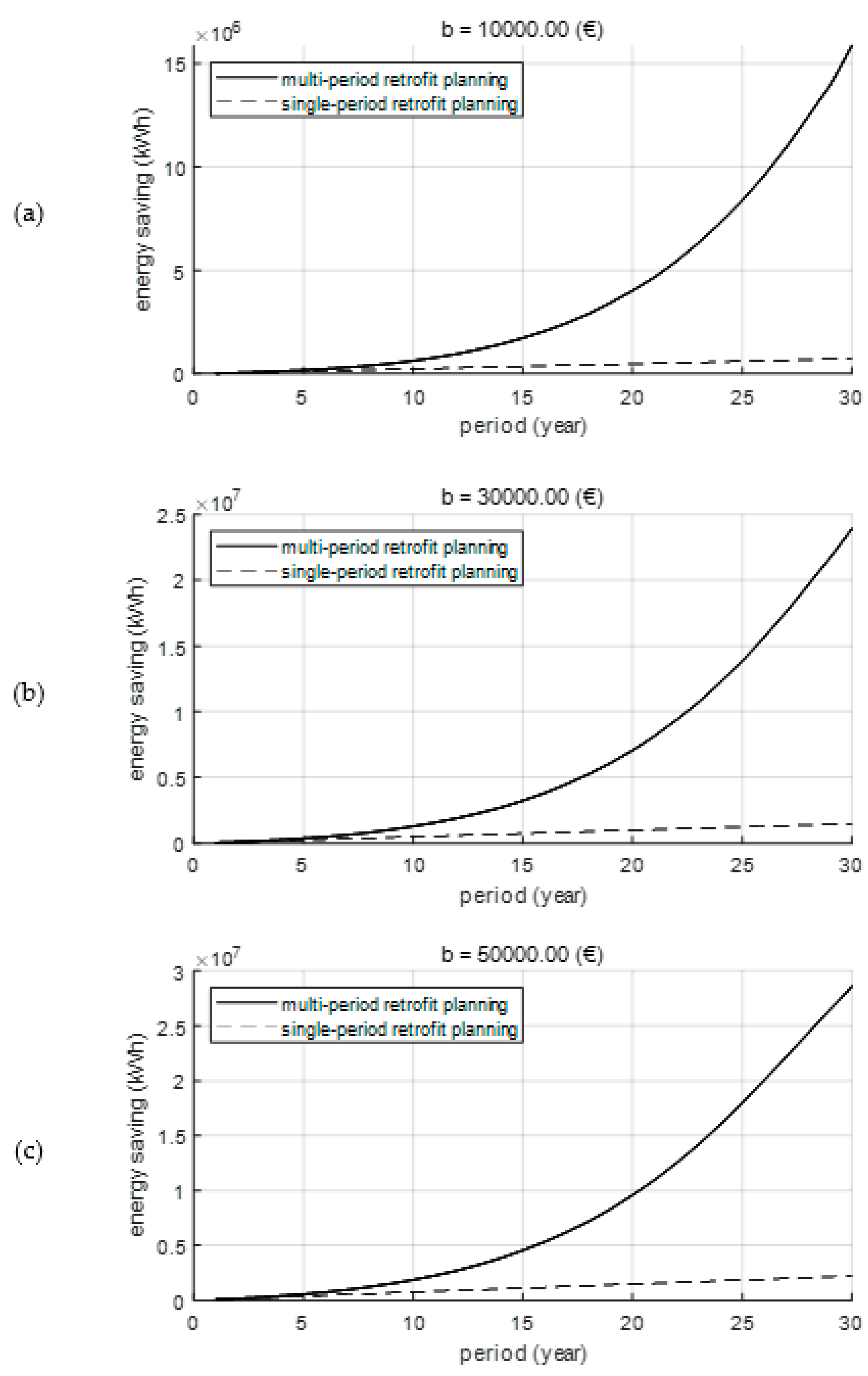
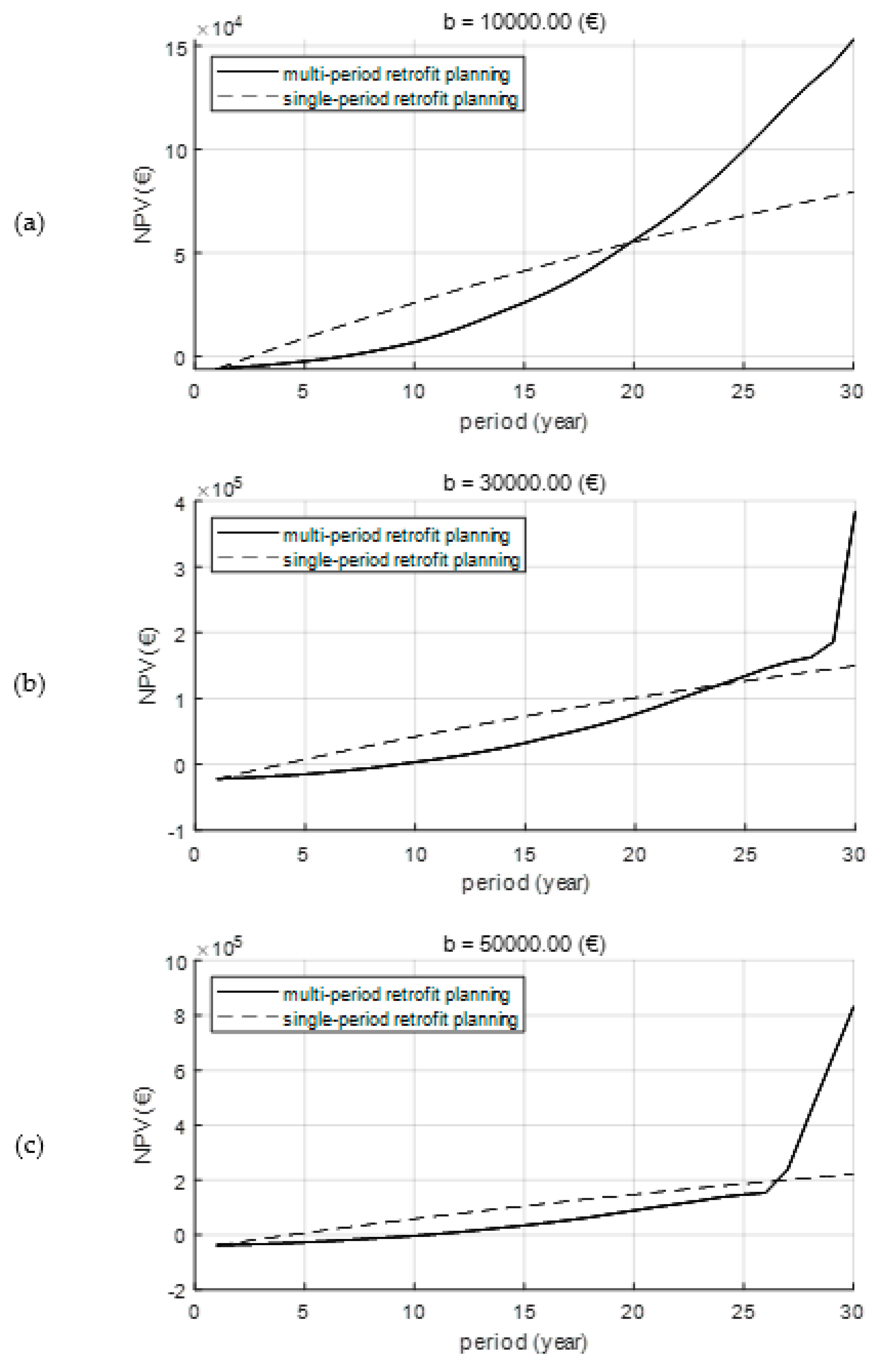
3.2. Energy Retrofit Results and Discussion

In this case study, we first give the analysis of this case in a single-period setting, and then extend the single-period model to a multi-period model considering different cases of analysis until K = 30 years. The single-period energy retrofit planning problem (4) presents 48 integer variables, 96 bounding constraints, and 1 inequality constraint, whilst the multi-period energy retrofit planning problem (15) presents 96 K integer variables, 192 K bounding constraints, $48K$ equality constraints, and K inequality constraints. The analysis of the widest planning horizon (i.e., K = 30) implies solving a problem with 2880 variables, 5760 bounding constraints, 1440 equality constraints, and 30 inequality constraints. In both settings, the problem is implemented and solved in the MATLAB environment integrated with IBM ILOG CPLEX Optimization Studio [34]. All the presented computations are executed on a PC equipped with a 4.0 GHz Intel Core i7 CPU and 16 GB RAM. The computational times are less than 1 minute in all the cases.

Figure 1 compactly reports the results of the planning problem in terms of retrofit actions in the case of initial investment budget $b$ = 30,000.00 (€) for both single- and multi-period (with K = 20 years) setting. Figure 1a shows the quantities of actions to be deployed normalized with respect to the application potentials. Conversely, Figure 1b shows the cumulative quantities of actions to be deployed, normalized with respect to the application potentials over the planning horizon. As expected, from Figure 1 it is evident that using a multi-period planning approach is more convenient than the single-period approach. In fact, after the initial investment, the subsequent savings in energy expenditures are used to accumulate cash to invest later in further energy retrofit actions, generating a beneficial snowball effect. More in detail, the single-period retrofit plan consists in implementing a limited set of actions (namely, retrofit actions $j\in \left\{11,15,18,19,20,21,22,28\right\}$) in Table 2, whilst the multi-period retrofit plan allows implementing a wider set of actions (namely, in addition retrofit actions $j\in \left\{1,6,26,27,31,32,36,37,42,45\right\}$) in Table 2. Specifically, the obtained multi-period retrofit planning consists of replacing a total of 379 luminaries with compatible LED lamps and installing a total of 926 EHMs, whilst the single-period retrofit planning consists of replacing 34 luminaries with compatible LED lamps and installing 1 EHM only.

To compare results in terms of overall achieved energy savings, and ensure the equality of conditions in the single- and multi-period setting, we consider an identical time window in both cases. Hence, we compare the total energy savings obtained by the multi-period optimization over the planning horizon $\mathcal{K}$ and the cumulative energy savings obtained by extrapolating the energy savings achieved by the single-period optimization in the initial period throughout the whole analysis time window $\mathcal{K}$. Denoting ${\mathit{x}}_1^{\ast },\dots ,{\mathit{x}}_k^{\ast },\dots ,{\mathit{x}}_K^{\ast }$ as the optimal retrofit plan computed by the multi-period approach—i.e., a solution of optimization problem (12)—the total energy savings achieved over the planning horizon $\mathcal{K}$ is expressed as:

$$E{S}_K^m={{\displaystyle \sum }}_{k=1}^K{{\displaystyle \sum }}_{j=1}^J{p}_{kj}{{\displaystyle \sum }}_{i=1}^k{x}_{ij}^{\ast }$$

(18)

where ${\mathit{p}}_k$ ($k=1,\dots ,K$) are the unitary payoff vectors estimated in accordance with (16). On the other hand, in case of single-period planning, denoting ${\mathit{x}}_1^{^}$—i.e., an optimizer of (4)—the total energy saving achieved at the end of time period K is computed as follows:

$$E{S}_K^s={{\displaystyle \sum }}_{k=1}^K{\mathit{p}}_k^T{\mathit{x}}_1^{^}.$$

(19)

Figure 2 shows the energy savings over the analysis time window achieved by the single- and multi-period retrofit planning for different initial investment budgets. It is apparent that the multi-period planning produces significantly higher energy savings for the same initial investment budget. For instance, the initial budget $b$ = € 10,000.00 yields a total energy saving of 0.7 MWh in $K$ = 30 years by using the single-period retrofit planning. This equals about one twentieth of the total energy savings achieved in the same time window for the same initial budget by using the multi-period retrofit planning (16 MWh). Finally, Figure 2 shows (as expected) that the deviation between results in the single- and multi-period planning is more marked for longer planning windows and lower initial investment budgets.

In order to further highlight the advantages of using a multi-period retrofit optimization approach over a single-period method, we also compare the net present values (NPVs) of the financial gains achieved when single- and multi-period retrofit planning techniques are used to maximize the energy savings. Indeed, NPV is used in the budgeting and investment planning phase as one of the most common profitability indexes for investment projects [35]. It is defined as the difference between the present value of cash inflows and the present value of cash outflows over a period of time [36]. Therefore, in the two cases of single- and multiple-time periods, NPVs are expressed as follows, respectively:

$$NP{V}_K^s=\left(b-{\mathit{c}}^T{\mathit{x}}_1^{^}\right)+{\displaystyle \sum }_{k=1}^K\frac{{\mathit{s}}_k^T{\mathit{x}}_1^{^}}{{{\displaystyle \prod }}_{i=1}^k\left(1+r_i\right)}-b$$

(20)

$$NP{V}_K^m=\frac{\left(b_K-{\mathit{c}}_K^T{\mathit{x}}_K\right)\left(1+r_K\right)+{\mathit{s}}_K^T{\mathit{z}}_K}{{{\displaystyle \prod }}_{k=1}^K\left(1+r_k\right)}-b.$$

(21)

where ${\mathit{c}}_k$ and ${\mathit{s}}_k$ ($k=1,\dots ,K$) are the unitary cost and cost energy savings vectors estimated by the corresponding models (9) and (13), and $r_k$ ($k=1,\dots ,K$) denotes the interest rate at time interval $k$.

Figure 3 shows the NPVs achieved by the single- and multi-period retrofit planning for different initial investment budgets. It is apparent that, considering a short planning horizon $K$ (i.e., less than 20, 24, and 26 years for an initial investment budget $b$ equal to €10,000.00, €30,000.00, and €50.000.00, respectively), the single-period approach has a higher NPV than the multi-period planning. This is caused by the fact that in the multi-period planning approach, the energy cost savings are invested in further retrofit actions. Conversely, substantial savings are obtained in the remaining part of the planning horizon in the multi-period approach. Hence, exceeding the above identified break point, the multi-period planning produces significantly higher NPVs for the same initial investment. For instance, the initial budget $b$ = € 10,000.00 yields NPVs equal to € 75,000.00 considering a time analysis window of $K$ = 30 years by using the single-period retrofit planning. This results about half the NPVs that are achieved considering the same time window for the same initial budget by using the multi-period retrofit planning (€ 150,000.00). Finally, Figure 3 shows that the deviation between results obtained in the single- and multi-period planning is more marked for longer planning windows and lower initial investment budgets.

The above numerical experiments carried out by varying the time horizon demonstrate that, while staging the interventions on the system may be a valuable strategy which allows savings to be obtained in several cases to (either energetical or economical), it might not be the best approach when the time horizon decreases. Hence, a proper assessment of the right strategy needs to be performed on a case by case basis.

4. Conclusions and Future Works

Given the considerable importance of consumption for urban street lighting in the energy and economic balance for many cities, in this work we focus on the selection of the optimal set of energy efficiency retrofitting interventions on public street lighting systems. Contrarily to classical approaches which optimize “one-off” interventions, our methodology defines a plan of retrofitting interventions which exploits the initial budget available for the investment as well as financial or environmental benefits and savings resulting from the implementation of energy efficiency measures. The application of the proposed methodology to a real street lighting system in the city of Bari, Italy, highlights the energy savings and financial benefits obtained by the multi-period planning instead of the classical single-period approach.

The contribution of the present research is twofold. First, we advance the existing literature on public street lighting by addressing a new topic, namely the multi-period approach for the development of the optimal plan of energy retrofitting interventions in urban street lighting. Second, we equip the city authorities in charge of energy efficiency and green energy for public lighting systems with a straightforward tool for defining the optimal plan of interventions focusing on the lighting system. In fact, a merit of the developed approach is its generalizability to different types of optimization criteria. Whilst in the current model we choose the total energy savings as the optimization criterion, an interesting development of the research can be to apply the retrofit decision-making model to optimize other indicators commonly used for assessing the energy performance of road lighting, and compare the insights that the model provides in these different scenarios.

This study is not without limitations. First, one can observe that input data frequently suffers from estimation uncertainties, and sometimes even very small errors could make the “optimal” retrofit solution irrelevant from the financial and environmental convenience perspective. Future research will be devoted to include uncertainty into the analysis. Second, public lighting systems are complex systems where retrofitting interventions produce a variety of consequences, related to economic, energy, environment and quality of life factors. Further research will address this issue by extending the analysis to a multi-objective problem. Third, the proposed approach has been developed from the standpoint of the public party who is in charge of the energy efficiency of lighting systems. Actually, very often, due to lack of expertise in public authorities and budget constraints, such interventions are carried out through innovative forms of collaboration with private parties (e.g., Energy Service Companies, typically called ESCOs), namely through public-private partnerships. Further work may also be done in this direction in order to include the two perspectives (i.e., public and private) in the model, thus providing a tool that is able to support the parties in the negotiation and contract design phases. Finally, one may observe that results and implications are derived from a specific and simple case study (where only LED and EHM are considered), since we assume that different retrofit actions produce additive effects on payoff and cost (i.e., we consider a linearly-constrained linear programming in the model). Actually, this limitation is only apparent, since the model can be easily generalized to complex cases with other objective and constraint functions to deal with the eventual and more complex refurbishment actions that would produce combined non-linear effects on the analyzed street lighting system.

References

1. Beccali, M.; Bonomolo, M.; Ciulla, G.; Galatioto, A.; Brano, V.L. Improvement of energy efficiency and quality of street lighting in South Italy as an action of Sustainable Energy Action Plans. The case study of Comiso (RG). Energy 2015, 92, 394–408. [Google Scholar] [CrossRef] [Green Version]
2. Pizzuti, S.; Annunziato, M.; Moretti, F. Smart street lighting management. Energy Effic. 2013, 6, 607–616. [Google Scholar] [CrossRef]
3. Richards, M.; Carter, D. Good lighting with less energy. Light. Res. Technol. 2009, 41, 285. [Google Scholar] [CrossRef]
4. Annunziato, M.; Honorato Consonni, C.; De Lia, F.; Fumagalli, S.; Giuliani, G.; Gozo, N.; Scognamiglio, A. LINEE GUIDA: I Fondamentali per una Gestione Efficiente Degli Impianti di Pubblica Illuminazione; ENEA: Roma, Italy, 2012. [Google Scholar]
5. The Covenant of Mayors. 2013. Available online: http://www.covenantofmayors.eu/index_en.html (accessed on 21 December 2018).
6. Popa, M.; Cepişcă, C. Energy consumption saving solutions based on intelligent street lighting control system. UPB Sci. Bull. Ser. C 2011, 73, 297–308. [Google Scholar]
7. Raciti, A.; Rizzo, S.A.; Susinni, G. Parametric PSpice Circuit of Energy Saving Lamp Emulating Current Waveform. Appl. Sci. 2019, 9, 152. [Google Scholar] [CrossRef]
8. Carli, R.; Dotoli, M.; Pellegrino, R. A decision-making tool for energy efficiency optimization of street lighting. Comput. Oper. Res. 2018, 96, 223–235. [Google Scholar] [CrossRef]
9. Cristea, M.; Tîrnovan, R.A.; Cristea, C.; Pică, C.S.; Făgărășan, C. A multi-criteria decision making approach for public lighting system selection. MATEC Web Conf. 2018, 184, 04006. [Google Scholar] [CrossRef]
10. Beccali, M.; Bonomolo, M.; Leccese, F.; Lista, D.; Salvadori, G. On the impact of safety requirements, energy prices and investment costs in street lighting refurbishment design. Energy 2018, 165, 739–759. [Google Scholar] [CrossRef]
11. Stuart, E.; Larsena, P.H.; Goldmana, C.A.; Gilliganc, D. A method to estimate the size and remaining market potential of the U.S. ESCO (energy service company) industry. Energy 2014, 77, 362–371. [Google Scholar] [CrossRef]
12. Suhonena Okkonenb, L. The Energy Services Company (ESCo) as business model for heat entrepreneurship-A case study of North Karelia, Finland. Energy Policy 2013, 61, 783–787. [Google Scholar] [CrossRef]
13. Carbonara, N.; Pellegrino, R. Public-private partnerships for energy efficiency projects: A win-win model to choose the energy performance contracting structure. J. Clean. Prod. 2018, 170, 1064–1075. [Google Scholar] [CrossRef]
14. Yao, Q.; Wang, H.; Uttley, J.; Zhuang, X. Illuminance Reconstruction of Road Lighting in Urban Areas for Efficient and Healthy Lighting Performance Evaluation. Appl. Sci. 2018, 8, 1646. [Google Scholar] [CrossRef]
15. Tan, B.; Yavuz, Y.; Otay, E.N.; Çamlıbel, E. Optimal selection of energy efficiency measures for energy sustainability of existing buildings. Comput. Oper. Res. 2016, 66, 258–271. [Google Scholar] [CrossRef]
16. Lauro, F.; Longobardi, L.; Panzieri, S. An adaptive distributed predictive control strategy for temperature regulation in a multizone office building. In Proceedings of the 2014 IEEE International Workshop on Intelligent Energy Systems (IWIES), San Diego, CA, USA, 8 October 2014; pp. 32–37. [Google Scholar]
17. Pellegrino, R.; Costantino, N.; Giustolisi, O. Flexible investment planning for water distribution networks. J. Hydroinform. 2018, 20, 18–33. [Google Scholar] [CrossRef]
18. Digiesi, S.; Facchini, F.; Mossa, G.; Mummolo, G.; Verriello, R. A cyber-based DSS for a low carbon integrated waste management system in a smart city. IFAC-PapersOnLine 2015, 48, 2356–2361. [Google Scholar] [CrossRef]
19. Dickinson, M.W.; Thornton, A.C.; Graves, S. Technology portfolio management: Optimizing interdependent projects over multiple time periods. IEEE Trans. Eng. Manag. 2001, 48, 518–527. [Google Scholar] [CrossRef]
20. Leccese, F.; Salvadori, G.; Rocca, M. Critical analysis of the energy performance indicators for road lighting systems in historical towns of central Italy. Energy 2017, 138, 616–628. [Google Scholar] [CrossRef]
21. Martello, S. Knapsack Problems: Algorithms and Computer Implementations; Wiley-Interscience Series in Discrete Mathematics and Optimization; Wiley: Hoboken, NJ, USA, 1990. [Google Scholar]
22. Wang, B.; Xia, X. Optimal maintenance planning for building energy efficiency retrofitting from optimization and control system perspectives. Energy Build. 2015, 96, 299–308. [Google Scholar] [CrossRef] [Green Version]
23. Carli, R.; Dotoli, M.; Pellegrino, R. A Hierarchical Decision Making Strategy for the Energy Management of Smart Cities. IEEE Trans. Autom. Sci. Eng. 2017, 14, 505–523. [Google Scholar] [CrossRef]
24. Ranieri, L.; Mossa, G.; Pellegrino, R.; Digiesi, S. Energy Recovery from the Organic Fraction of Municipal Solid Waste: A Real Options-Based Facility Assessment. Sustainability 2018, 10, 368. [Google Scholar] [CrossRef]
25. Bruno, S.; D’Aloia, M.; De Benedictis, M.; Lamonaca, S.; La Scala, M.; Rotondo, G.; Stecchi, U. Studio di Fattibilità per la Integrazione di un Modello di Pubblica Illuminazione ad Alta Efficienza in un Power Park Urbano (Quartiere Eco-Sostenibile): Analisi di un Caso Pilota. 2011. Available online: http://www.enea.it/it/Ricerca_sviluppo/documenti/ricerca-di-sistema-elettrico/smart-city/rds-328.pdf (accessed on 21 December 2018). (In Italian).
26. European Committee for Standardization. EN 13201e2. Light and Lighting. Road Lighting—Part 2: Performance Requirements; European Committee for Standardization: Brussels, Belgium, 2015. [Google Scholar]
27. European Committee for Standardization. EN 13201e2. Light and Lighting. Road Lighting—Part 3: Calculation of Performance; European Committee for Standardization: Brussels, Belgium, 2015. [Google Scholar]
28. European Committee for Standardization. EN 13201e4. Light and Lighting. Road Lighting—Part 4: Methods of Measuring Lighting Performance; European Committee for Standardization: Brussels, Belgium, 2015. [Google Scholar]
29. Rea, M.S. The IESNA Lighting Handbook; Illuminating Engineering Society of North America: New York, NY, USA, 2000. [Google Scholar]
30. Lagorse, J.; Paire, D.; Miraoui, A. Sizing optimization of a stand-alone street lighting system powered by a hybrid system using fuel cell, PV and battery. Renew. Energy 2009, 34, 683–691. [Google Scholar] [CrossRef]
31. Lighting Products Catalog. Available online: http://www.lighting.philips.com/main/systems/system-areas/roads-and-streets (accessed on 21 December 2018).
32. List of Prices for Public Works in Apulia Region. Available online: http://www.regione.puglia.it/elenco-prezzi-2017 (accessed on 21 December 2018). (In Italian).
33. Eurostat, Electricity Prices for Non-Household Consumers—Bi-Annual Data. Available online: http://appsso.eurostat.ec.europa.eu/nui/submitViewTableAction.do (accessed on 21 December 2018).
34. IBM. IBM ILOG CPLEX Optimization Studio Getting Started with CPLEX for MATLAB. Available online: https://www.ibm.com/support/knowledgecenter/en/SSSA5P_12.6.2/ilog.odms.cplex.help/CPLEX/MATLAB/topics/gs.html (accessed on 21 December 2018).
35. Brealey, R.; Myers, S. Principles of Corporate Finance; McGraw-Hill: Irwin, PA, USA, 2000. [Google Scholar]
36. Jain, P.K. Theory and Problems in Financial Management; Tata McGraw-Hill Education: New Delhi, India, 1999. [Google Scholar]
Figure 1. The cumulative energy savings over time intervals achieved by single- (a) and multi-period (b) retrofit planning for an initial investment budget b = € 30,000.00.
Applsci 09 01025 g001
Figure 2. The cumulative energy savings over time intervals achieved by single- and multi-period retrofit planning for different initial investment budgets: (a) b = € 10,000.00, (b) b = € 30,000.00, and (c) b = € 50,000.00.
Applsci 09 01025 g002
Figure 3. The NPVs over time intervals achieved by single- and multi-period retrofit planning for different initial investment budgets: (a) b = € 10,000.00, (b) b = € 30,000.00, and (c) b = € 50,000.00.
Applsci 09 01025 g003