1. Introduction
Energy utilization efficiency is increasing with increased use of technology and smart appliances in every field of life in the residential, commercial and industrial sectors. At the same time, a reliable and high-quality electrical power system is extremely vital to fulfil the residential energy demand. Meanwhile, there is a rapid increase in demand for global natural resources. Throughout the world, major blackouts occur due to consumer demand and utility supply mismatch and system automation deficiencies. Hence, a transition process from the Traditional Electric Power Grid (TEPG) to the Smart Grid (SG), to integrate communication and information technologies, is the demand of the future. Presently, about 40% of the total generated energy is consumed by residential users, and approximately 30–40% of carbon emission is due to these residential areas [
1]. The unnecessary and inefficient use of electrical energy brings sustainability issues to the forefront, such as economic growth, heavy pollution and global warming. Conventionally, the service provider power systems run on fossil fuel and add to global warming with high carbon emissions. Furthermore, in the present power systems, electricity power flow is uni-directional, i.e., from the supply- to the demand-side. Conversely, SG’s purpose is to make the flow of electricity supply and demand bidirectional [
2]. Secondly, the search for and integration of new green renewable energy resources are obligatory in such circumstances. The integration of green renewable energy resources needs a broader perspective of design, planning and optimization. Up to this time, different conventional optimization techniques, such as Linear Programming (LP) [
3], Non-Linear Programming (NLP) [
4], Integer Linear Programming (ILP) [
5], Mixed Integer Linear Programming (MILP) [
6], Dynamic Programming (DP) [
7] and Constrained Programming (CP), have been practised. However, in the present situations, the integration of renewable energy resources is mandatory, and the problems are non-linear and have numerous local optima, making conventional optimization techniques obsolete. In the last decade, bio-inspired modern heuristic optimization techniques have grown in popularity due to their stochastic search mechanisms and avoidance of large convergence time for the exact solution [
1].
In this research work, we propose a new meta-heuristic optimization algorithm, named Time-constrained Genetic-Moth-Flame Optimization (TG-MFO), and applied it for efficient energy optimization in smart homes and buildings. We have also explored and analysed five bio-inspired heuristic algorithms for the energy optimization problem, namely the ACO, GA, Cuckoo Search Algorithm (CSA), Firefly Algorithm (FA) and MFO algorithms. For analysis and validation of the proposed algorithm, we applied these algorithms in different consumer scenarios, such as a single home for one day, a single home for thirty days, thirty different sizes of homes for one day and thirty homes for thirty days. Simulation results show that our proposed algorithm reduced the end-user discomfort in terms of appliance waiting time being nearly equal to zero, as compared to the bio-inspired optimization algorithms, along with minimization of total energy cost and minimum PAR. Renewable energy sources are also integrated for further minimization of the total load and its cost.
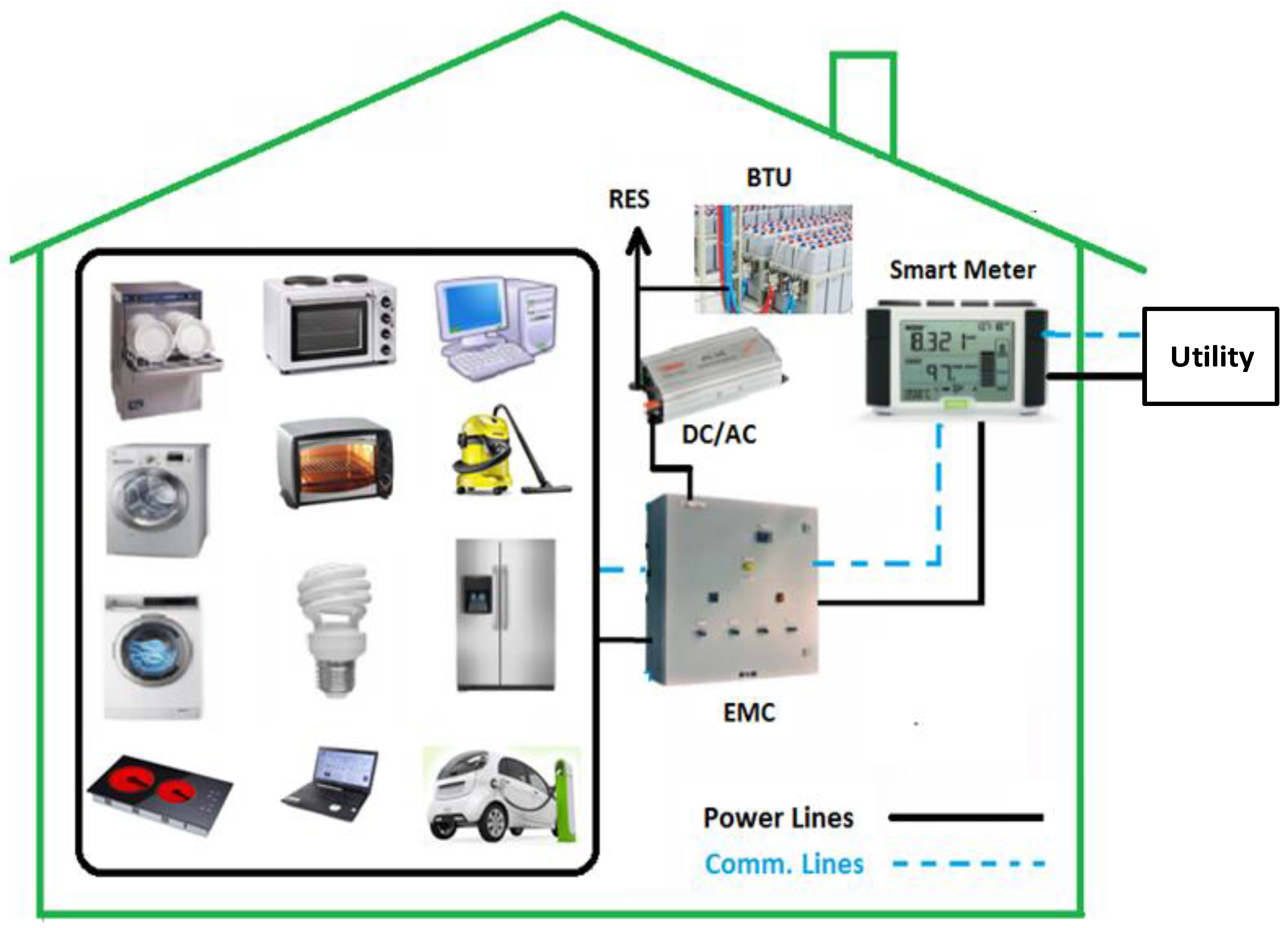
To achieve this goal, the smart electric grid is modelled as a residential sector comprised of 30 homes having different sizes, different Lengths of Operational Time (LOTs) and appliance power ratings. Appliance power ratings are different due to the home size requirements. For example, a small-sized home runs a one-ton (12,000 BTU) air conditioner compared to a large-sized home that runs 1.5 tons (18,000 BTU) or even more. Some homes have a Renewable Energy Source (RES) and a Battery Storage Unit (BSU). In the considered model, we have forty-eight (48) Operational Time Intervals (OTIs) in a day, by dividing one hour into two-time slots of thirty minutes each. In each OTI, a smart home checks appliances’ power demand, i.e., whether an appliance is ON or OFF. According to the appliances’ ON/OFF status, the Energy Management Controller (EMC) checks the availability of RES and BSU to fulfill the appliances’ power demand. If it is available, the appliance will be ON, and the consumer will not wait for appliance scheduling. If the generation and stored energy are insufficient for running the load, the proposed algorithm will check the time span, in which a user has no problem with appliance scheduling with the lowest energy price (time interval) for running that appliance. In order to achieve this objective, time constraints have been defined for a maximum interval of time in which an appliance has to complete its operation. Consequently, if the utility gives incentives to the user in the form of real-time lower prices in off-peak hours, the end-user will be encouraged to produce his/her own energy from RES and schedule the load accordingly. The rest of the paper is organized as follows: Related work is illustrated in
Section 2. Contributions are briefly discussed in
Section 3.
Section 4 depicts the proposed system model architecture. The problem formulation is described in
Section 5, and
Section 6 gives the heuristic algorithms.
Section 7 presents the simulation results to demonstrate some of the achievements. The paper is concluded in the last section.
2. Related Work
Countless researchers around the world are investigating different technologies in order to fulfill the needs of energy-efficient and intelligent smart homes. Many algorithms have been proposed for optimal use of existing energy resources. In this regard, we illustrate some prior research works in SG.
Yi Peizhong et al. [
8] have proposed the Optimal Stopping Rule (OSR) for energy-efficient scheduling of home appliances. The limitation of this work is that OSR runs on a threshold-based strategy. The end-user has to wait until the price comes down below the threshold level. In [
9], the authors have proposed an approach to optimize their objective function using the Genetic Algorithm (GA). Electricity prices are varying between on-peak hours and off-peak hours. Therefore, an optimized task scheduling module is used in smart homes, which can reduce the consumption of the entire energy and operation times. Having an optimal scheduling of power, a heuristic-based GA was used for Demand-Response (DR) in Home Energy Management (HEM) systems in [
10]. The authors proposed GA-, TLBO- (Teaching Learning-Based Optimization), EDE (Enhanced Differential Evolution) and EDTLA- (Enhanced Differential Teaching Learning-based Algorithm) based approaches, which are used for minimization of the residential total energy cost and maximization of the end-user comfort level.
The problem of optimal scheduling of household appliances has been explored in [
11]. The authors used the day-ahead changeable peak pricing technique for the minimization of the consumer’s energy consumption cost using a combination problem approach. This approach enables customers to schedule their household appliance using MKP (Multiple knapsack problem) formulation. In [
12], the authors implemented GPSO (Gradient-based Particle Swarm Optimization) for DR in smart homes by considering load and energy price uncertainties. The authors employed GA and BPSO (Binary Particle Swam Optimization) for optimal scheduling of home appliances in [
13]. They proposed GAPSO (Genetic Algorithm with Particle Swam Optimization), a hybrid scheme of both these techniques, to obtain better results in terms of reducing PAR, minimization of electricity cost and especially end-user discomfort. Day-Ahead Pricing (DAP) and Critical Peak Pricing (CPP) are used as pricing schemes for single and several days. The authors used GA and TLBO and their hybrid TLGO (Teacher Learning-based Optimization with Genetic algorithm) for appliance scheduling in [
14]. They categorized flexible appliances as time flexible and power flexible for proficient energy consumption of consumers in SG. This approach enables energy consumers to schedule their appliances to obtain optimized energy consumption. This approach also maximizes the comfort level of customers with restricted total energy consumption. The authors in [
15] discussed the strategy for scheduling appliances in order to reduce carbon emissions along with the reduction of the electricity bill and waiting time. They applied the cooperative multi-swarm PSO technique to achieve their goals; however, they did not consider PAR. The authors implemented the 0/1 multiple knapsack problem with the genetic algorithm to find a good solution in [
16]. A simple fitness function is evaluated for each appliance in every time slot to obtain the desired results. The authors proposed a Demand-Side Management (DSM) strategy. This technique is based on a load shifting strategy during peak hours to reduce electricity bills using an Evolutionary Algorithm (EA). The authors discussed the strategy of the load shifting-based generalized technique, from on-peak hours to off-peak hours of a day, to minimize energy cost. This mechanism can support a large number of controlled devices of numerous types to minimize end-user electricity bills.
An adaptive energy model for DSM in smart homes has been proposed by the authors in [
17]. Distributed RESs’ usage is optimized using the ACO algorithm. In [
18], Kusakana et al. used the TOU pricing model along with the integration of RESs and BSUs to minimize the end-user’s electricity bill and achieve energy consumption balancing. The authors proposed a model to sale extra generated energy back to the utility, as per their prior agreement. For minimization of the end-user electricity bill, Bharathi et al. suggested a model in [
19], which works in industrial, commercial and residential areas. For optimization, the authors used GA. They also compared the different EA with GA and found that it gave a maximum decrease of 21.9% in the consumption of energy.
In [
20], the authors proposed objective function generalization using the DR program to minimize the residential consumer electricity bill. The authors showed that by shifting the load, unexpected peaks were observed in off-peak hours. They evaluated this later peak formation with multi-CPP and multi-TOU pricing schemes combined with DAP concepts. In [
21], in order to lessen the end-user electricity cost and minimize the end-user discomfort, Ogunjuyigbe et al. developed a GA-based optimization technique for scheduling of appliances.
In [
22], authors presented a DSM strategy, by shifting the load from on-peak hours to off-peak hours, using DAP signal and Evolutionary Algorithm (EA). However, consumer comfort is not considered. In [
23], the authors proposed a Quality of Experience (QoE)-based home energy management system. They gave the priority to the end-user’s frustration. Two algorithms that run the HEM system are: “QoE-aware Cost Saving Appliance Scheduling (Q-CSAS)” for scheduling of controlled load and “QoE-aware Renewable Source Power Allocation (Q-RSPA)” for management of appliances for renewable energy sources’ surplus energy. They reduced energy cost to 30–33% without RES and 43–46% with RESs for the end-user annoyance rates of 1.67–3.36 and 1.70–3.43, respectively. In [
24], the authors introduced three heuristic-based algorithms: GA, ACO and BPSO, to maximize user comfort, minimize PAR and minimize electricity cost, as well. In [
25], the authors proposed a hybrid GA-PSO, which is a combination of the GA and PSO algorithm, for energy management and obtaining maximum end-user comfort in smart homes. K. Muralitharan et al. [
26] presented multi-objective EA for the minimization of electricity bill and appliances waiting time. As soon as the running appliances’ load increases from a threshold, they are switched off. A multi-residential energy scheduling issue with multi-class appliances in a smart grid was discussed in [
27]. The authors proposed a PL-generalized Benders algorithm (Property (P) and L-Dual-Adequacy) for bill minimization and bounded user comfort. In [
28], the authors proposed a distributed algorithm for shifting the load from on-peak hours to off-peak hours. They used the game theory approach for scheduling the residential load. The Nash equilibrium convergence rate was also accelerated by the Newton technique. PAR and end-user discomfort were minimized.
The aforementioned research works achieved the cost minimization and reduction of PAR at the cost of end-user’s waiting time. Therefore, in this paper, using TG-MFO, we achieved a nearly-zero waiting time along with cost and PAR minimization.
Table 1 depicts the achievements and limitations of the aforementioned research work.
5. Problem Formulation
In this work, we assumed a single home and thirty homes with different power ratings of appliances, as tabulated in
Table 2. Our required objectives are:
- (a)
Consumers’ high comfort level by reducing appliances’ average waiting time,
- (b)
Consumers’ electricity bill minimization,
- (c)
Minimization of PAR and
- (d)
Integration of RES and BSU in the system for further reduction of end-user waiting time.
These objectives can be achieved by the optimization of the energy consumption profiles of home appliances, using different scheduling techniques. If is the maximum energy capacity in every time slot, then the end-user electricity cost along with PAR can be minimized, keeping aggregated energy consumption of cumulative home appliances within the maximum threshold limit of .
Mathematically, this constraint can be shown as follows:
Here, is the total energy demand of the end-user.
5.1. PAR
The peak to average ratio can be minimized, using the scheduling algorithms, which is in favor of both the utility and consumer for maintaining demand-supply balance. It is the ratio of the peak load of the consumer to the average load of the consumer, in every interval of time, and is denoted by
. Mathematically, it is defined as in [
33]:
5.2. User’s Comfort in Terms of Waiting Time ()
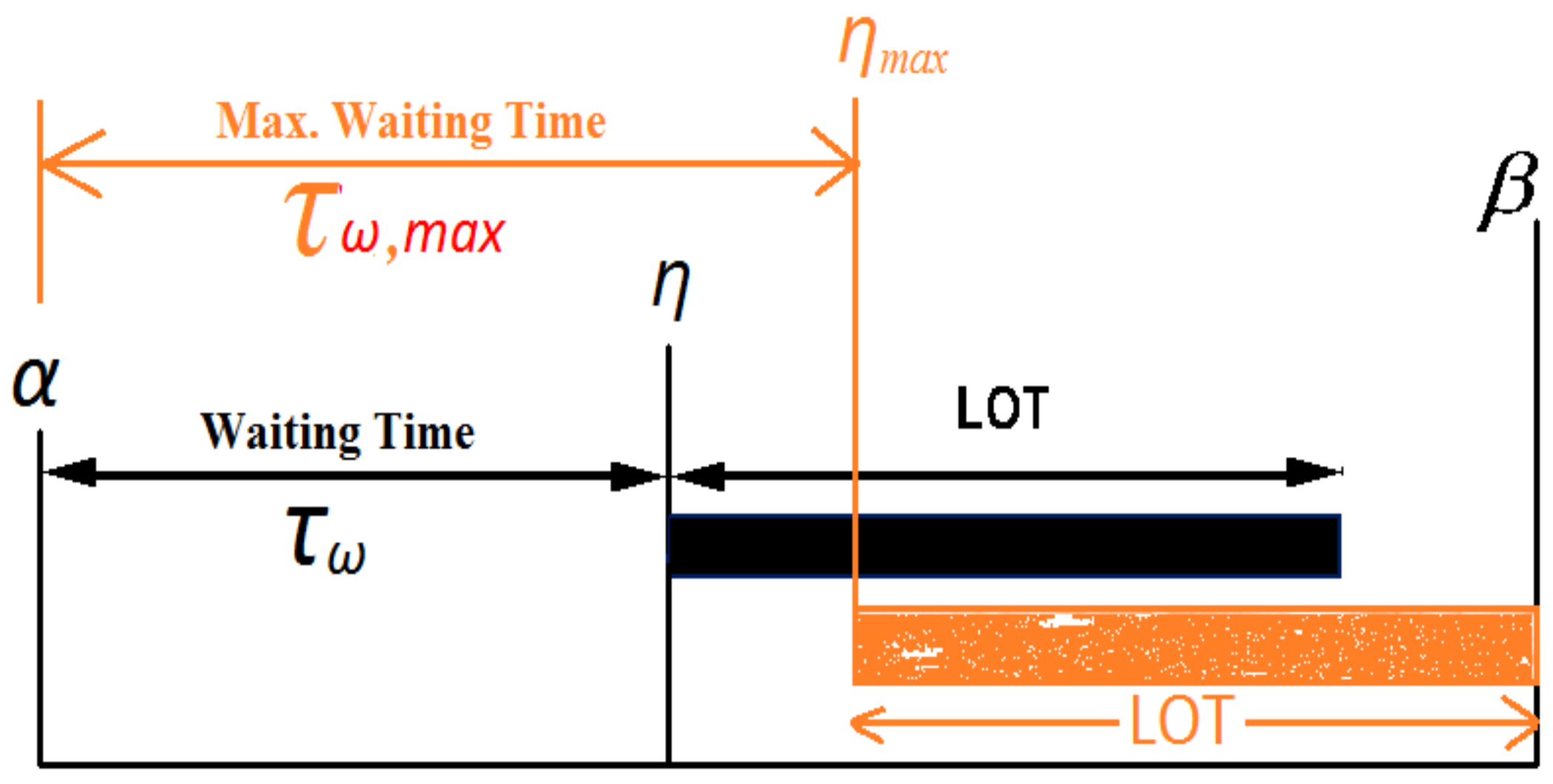
User’s comfort in terms of waiting time is important for end-users. Waiting time must be minimized to have a high comfort level so that the end-user’s frustration can be avoided. It is that interval of time when a consumer switches on an appliance, and due to the scheduling limitations of the system, he/she has to wait to start its operation. As we have defined the earliest starting time
and the latest ending time
of an appliance, then another parameter
will be the operational starting time of the same switched-on appliance. This is shown diagrammatically in
Figure 3. Here,
-
is the time span, defined by the consumer, as given in
Table 2.
Figure 3 shows that a consumer’s maximum waiting time could be up to
. Since LOT is already defined by the consumer, so at
, the algorithm will have to start the appliance to complete its operation up to the final time
. For example, Dishwasher-1 (
Table 2) has a time span of 8 h (from 9:00–17:00) and LOT = 2 h. This means that our proposed algorithm (TG-MFO) must start Dishwasher-1 from 9:00–17:00 to complete its operation of 2 h, with a waiting time ranging from 0–6 h.
Here, LOT is the length of the operational interval of time, in which an appliance completes its task. In the case of fixed appliances, there is no issue of waiting time, as whatever time the consumer wants to switch it on, he/she can do so. Therefore, we do not include fixed appliances in the scheduling problem.
Therefore, the range of waiting time can be
to
, as shown in
Figure 3.
Appliances’ normalized waiting time (
) can be calculated as:
Equation (
14) shows that the normalized waiting time can be from “0” (when
) to “1” (when (
).
Table 2 illustrates the typical electricity demand of a single home and multiple homes, with different power ratings and types of appliances, their LOTs and (
) and (
) constraints [
31]. Since different end-users have different habits and life routines, with different sizes and power ratings of appliances, we have assumed four (4) types of homes and randomly selected through the proposed algorithm, to have randomness in the consumed energy when taking multiple (here, 30) homes.
5.3. Objective Function
Mathematically, our objective function can be formulated as follows:
where
is the energy cost in every interval of time. Our proposed objective function aims to reduce electricity cost, while maintaining a higher end-user comfort level by minimization of waiting time.
and
are multiplying factors of two portions of the objective function. Their values can be either “0” or “1” so that (
+
) = 1 [
24]. This reveals that either
and
could be 0 or 1. That is, if a consumer does not want to participate in the load scheduling process, then his/her multiplying factors will be
= 1 and
= 0 in the objective function.
6. Scheduling Algorithms
Heuristic means “to discover”, or “to find” or “to hit upon” by experiment, trial and error approaches. The solution of an optimization problem can be found in a realistic interval of time. However, such optimization techniques cannot guarantee the optimal solution. Meta-heuristic means “to find on a higher level” or “to find ahead of” local optimization. This means its performance is superior to straightforward heuristics techniques. All such algorithms use the process of local search and randomization, which further provides a path to global search and optimization.
The problem of scheduling home appliances optimally, using different meta-heuristic algorithms like GA, ACO, FA, MFO and CSA, is discussed in
Section 6. Various classical programming techniques like LP, ILP, MILP, DP and CP have already been used by researchers for optimal scheduling of home appliances. The convergence time of these classical techniques is very large due to the exact solution, and to schedule a large number of appliances, they cannot be used. Furthermore, classical algorithms usually show the best results for local optimization, as compared to the global point of view. Therefore, due to their probabilistic nature, bio-inspired meta-heuristic algorithms give good results in the case of local, as well as global solutions.
6.1. GA
GA is in the family of evolutionary algorithms. This algorithm’s name is due to it being inspired the genetic progression of living organisms. It has a quick rate of convergence. GA carries out parallel search operations in the provided solution space, which reduces the chances of being trapped in the local optimal solution. For complex non-linear problems’ formulation, GA is the best option, especially where the global optimization is a challenging job. For any solution deployment, as GA is probabilistic in nature, the optimality is usually not guaranteed [
34].
GA initiates a random population known as chromosomes, and then, in every iteration, the generated population is updated. Home appliances are mapped with bits of chromosomes. The fitness function of a given problem is evaluated by the suitability of each chromosome. In every iteration, the population is updated by storing the present local best solution, known as elitism. After elitism, in order to reproduce new chromosomes, two parent chromosomes are chosen using the tournament-based selection technique. Then, on the basis of selected chromosomes, the crossover procedure is performed. New offspring are added to update the present population [
35].
Table 3 shows the GA parameters.
6.2. MFO
The nature-inspired algorithm MFO was proposed by Seyedali Mirjalili in 2015 [
36]. Moths are butterfly-like insects, having 160,000 plus different species in nature. They have their unique navigation mechanism known as transverse orientation when flying in the moonlight. When they fly in a spiral, they maintain a constant angle related to the moon, ultimately converging in the direction of light. The spiral articulates the searching region, and it assures the exploitation of the optimum solution.
Since MFO is a population-based algorithm, the movement of m moths in n dimensions (variables) is given in the position matrix form as follows:
The resultant fitness values, for “m” number of moths, are stored in an array. The fitness function (objective) evaluates each moth’s fitness value. Each moth’s position vector, i.e., matrix Q’s first row, is evaluated on the fitness function, and its output is then allocated to its respective moth.
Similarly, a matrix
is assigned to the corresponding flames as follows:
Now, in mapping our problem of the optimum scheduling of home appliances, moths act as searching agents, and flames are the optimum positions. In each iteration, a moth searches for an optimum flame, with updates in the next iteration for the best solution by comparing with the previous one. Moths follow the logarithmic spiral for their update positions, where moths start from some initial position, following some limited fluctuating search space, and reach their destination flames. In MFO, the logarithmic spiral is:
where
is the
moth distance from
flame,
b is the spiral shape defining the constant and the random number t lies between −1 and one. When
, this means the moth is closest to its destination flame, while
indicates that its farthest position from the flame. Therefore, the moth is always assumed to be in a hyper-ellipse space, which guarantees the exploitation and exploration of search space.
Table 4 depicts the MFO parameters.
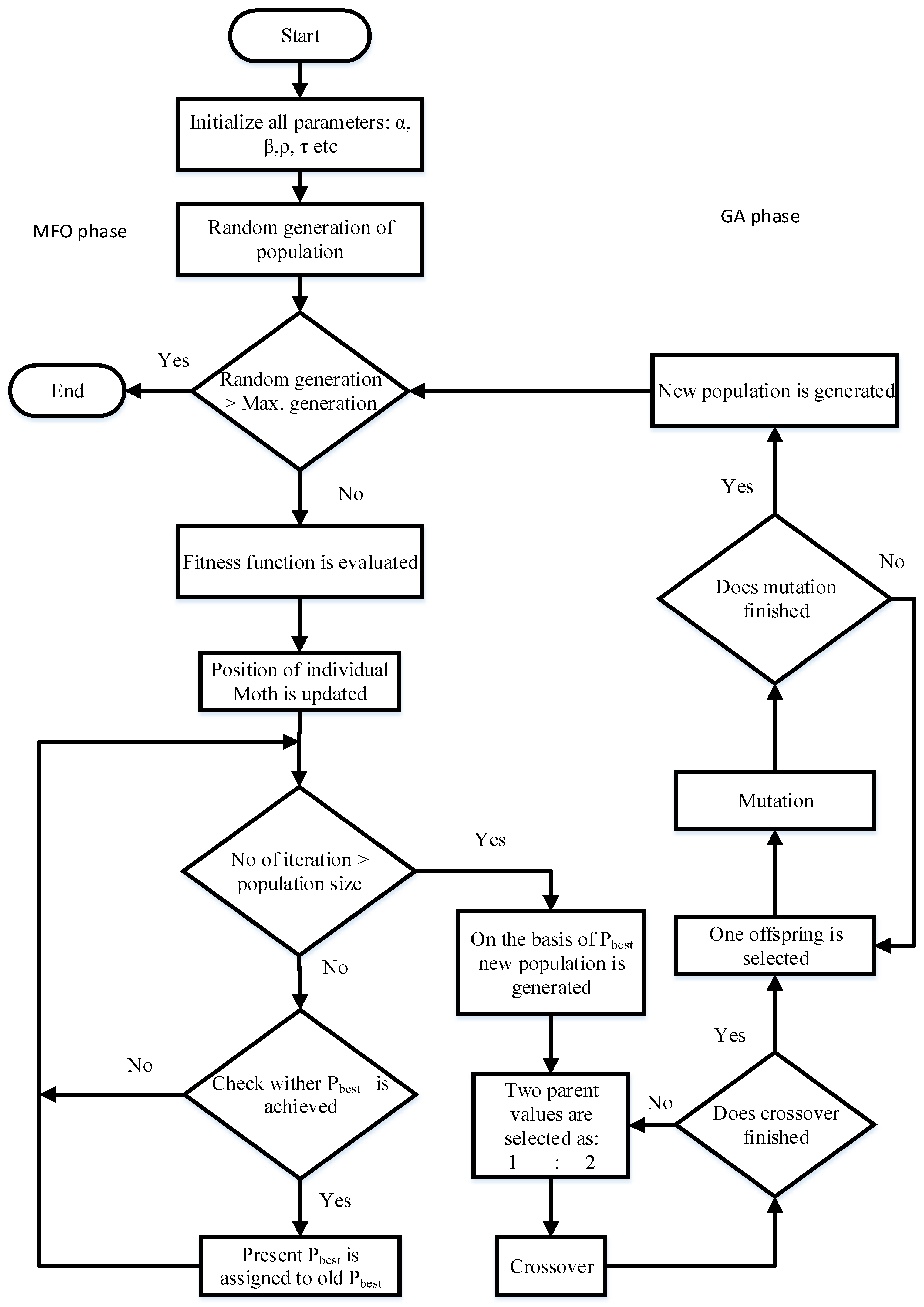
6.3. TG-MFO
In this work, we apply the bio-inspired algorithms GA, MFO and their hybrid version TG-MFO. Then, we compare their results with some of the existing techniques like ACO, CSA and FA on randomly-generated data. Then, we apply the strategy of the time constraints of end-users, i.e., for each appliance to switch-ON, we give some time span as the initial and final thresholds for all appliances. A user initiates the operation of an appliance, but usually, it is allowed to remain OFF for a certain time interval, in which the user has no problem or frustration. We apply this time threshold policy, to have a zero end-user waiting time. TG-MFO is based on the hybridization of GA and MFO with time constraints. Initially, MFO is applied on randomly-generated data for the optimization problem to obtain the local best positions for home appliances. Then, GA is applied to compare MFO’s local best solution with the new random data, to find the global best solution in each iteration. The fitness functions are updated accordingly. This process continues until the termination criterion is fulfilled.
Figure 4 depicts the steps involved in the TG-MFO implementation process, while, the pseudocode of Algorithm 1 shows the step-by-step working of the proposed TG-MFO algorithm.
6.4. ACO
ACO is a bio-inspired meta-heuristic iteration-based optimization technique. Using pheromone trails, chemicals as signals to other ants left on the ground known as the Stigmergy principle, starting from their nest, in search of food, ants find the shortest routes between their origins to the destination. If an ant wants, with a certain probability, to follow a particular path, it follows the pheromone trail. It reinforces the other ants by laying more pheromone on the same trail. As the movement of ants increases on a route, the amount of pheromone increases. Since pheromones’ nature is volatile, so the shortest path has more pheromone as compared to the longer one. As a result, ants’ movement increases on the shortest route.
Using this principle, ACO is used for the solution of discrete combinatorial search optimized-solution problems. Self-organization and self-healing are the distinguishing properties of ACO. ACO is used for the residential consumer’s energy optimization, which is a novel scheme for such energy management problems [
24]. The ACO parameters are given in
Table 5.
| Algorithm 1: Pseudocode of the proposed TG-MFO algorithm. |
![Applsci 09 00792 i001]() |
6.5. CSA
The cuckoo search algorithm was proposed by [
37] and belongs to the family of bio-inspired meta-heuristic algorithms. It is used to solve the optimization problems using the mating and production behaviour of some cuckoo species and the characteristics of Lèvy flights of some birds and fruit flies. Certain cuckoo species use nests of other birds to lay their eggs, selected randomly, known as host nests. The birds who own these nests may find these eggs and raise the cuckoo’s young. CSA uses certain rules to find the best local solution by mapping pattern of eggs (1,0) with home appliances’ ON-OFF condition, stated as follows:
The nest is randomly selected, in which each cuckoo lays one egg at a time.
For upcoming production, those nests will be selected having the higher quality eggs.
The host bird determines that the cuckoo laid the eggs, while the number of host nests is fixed.
The algorithm starts the discovery of the local best solution from randomly-given eggs (either one or zero) in the host nests. This one or zero shows the ON and OFF states of home appliances to be scheduled in a given time-slot. According to the fitness function, each egg (probable solution) is assessed. This solution will be our objective of minimum cost and PAR with reduced waiting time constrained. The production step is repeated, while discovering the superior eggs with a probability of 0.25. Lèvy flights are carried out to find the global best solution, out of the local best solution [
38].
Table 6 gives the CSA parameters.
6.6. FA
Fireflies are in the insect family. They live mostly in humid environments. They generate green, yellow and pale-red limited intensity flashing lights chemically. There are more than 2000 different species. Their unique flashing light pattern is used for communication, i.e., to attract partners and probable prey and as a defensive cautionary mechanism. Some female species apply the flashing light mating pattern for the hunting of other species [
39].
Like PSO, in FA, inspired by nature, three assumptions are made: (a) all fireflies must be of the same sex, (b) the attractiveness of a firefly is directly proportional to its brightness and inversely proportional to the square of the distance between two fireflies and (c) brightness is calculated by an objective function: the brighter one will attract the less bright ones. The firefly’s flashing light intensity in complete darkness is related to the solution quality. The brighter firefly will attract less bright ones, depending on the brightness intensity, which is calculated as follows:
where
is the flashing light intensity at the origin and
is the distance of firefly
j from firefly
i. Let
be the coefficient of the firefly’s flashing light absorption in a medium, then, in the above equation, the light intensity
I will vary with the distance between fireflies
using the following equation:
Both Equations (19) and (20) can be combined using the Gaussian form as follows:
The following approximation can be used for a slower rate of decrease in the light intensity between the origin and the target.
As the less bright firefly will be attracted to the brighter firefly, this attractiveness
between two fireflies can now be mapped as:
where
is the attractiveness at the zero distance. For
at the zero distance,
Therefore, for a characteristic distance of
, Equation (
23) becomes:
The distance between any two fireflies
x and
y at positions
i and
j is calculated by:
The firefly movement towards another firefly has two parts:
- (a)
The movement will be for finding a better solution using attractiveness.
- (b)
The movement will be random.
where
is the randomness parameter and
is a random number generated lying between zero and one. Two extreme points are that when
is zero, attractiveness will be constant, and when
is
∞, attractiveness will almost be zero. Practically,
lies between zero and
∞, so FA gives good results in finding local, as well as global optima [
39].
Table 7 depicts the FA parameters.
7. Results and Discussions
7.1. Consumer Scenarios
In the present work, four types of consumer scenarios were simulated and discussed. In the first case, a single home was taken, and its hourly load, hourly energy cost, PAR and waiting time were determined both in the unscheduled and scheduled (with ACO, CSA, GA, FA, MFO and TG-MFO) environment for a single day. In the second case, a residential building with thirty homes having users with different habits with different LOTs and different power ratings of appliances were considered. Again, their hourly average load, hourly cost, PAR and waiting time were determined both for unscheduled and scheduled (with ACO, CSA, GA, FA, MFO and TG-MFO) scenarios for a single day. In the third case, we considered a single home, found all four of its parameters for unscheduled and scheduled scenarios for a complete month, i.e., thirty (30) days, and found its monthly bill. In the fourth case, a residential building with thirty homes was considered, and we determined its daily average load, daily cost, daily PAR and average waiting time for a complete month, i.e., thirty (30) days, as well as calculated its monthly electricity consumption and electricity bill. In all four cases, the RTP scheme was used.
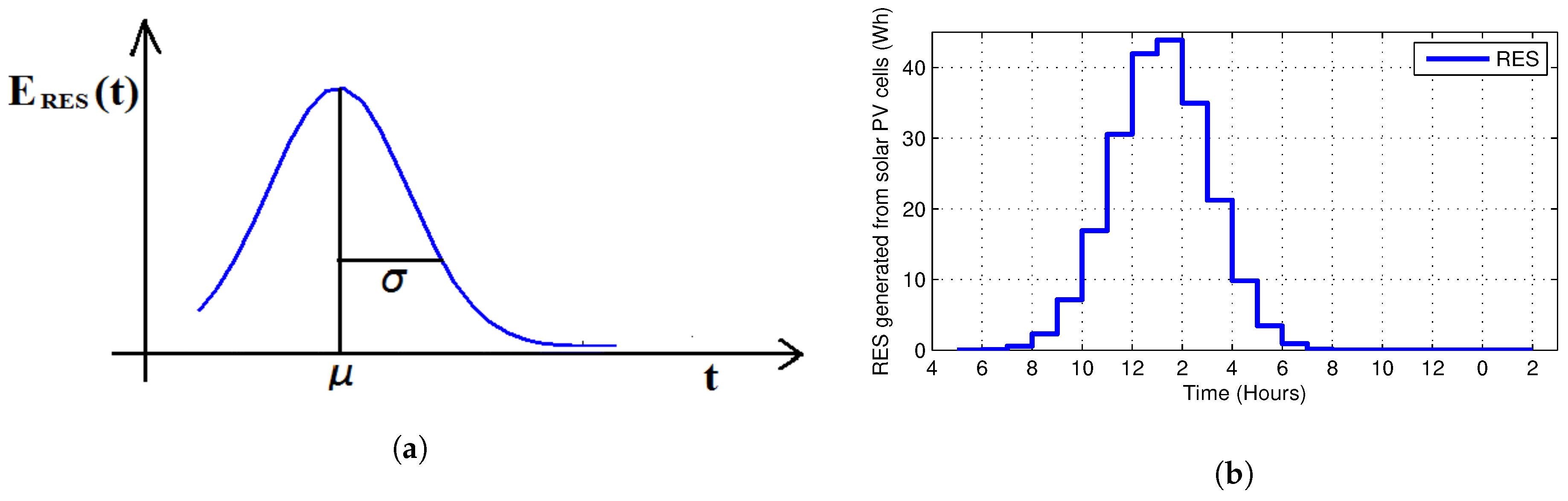
For the system’s stability, further reduction of electricity consumption and maximum user comfort, RES and BSUs were also integrated. Additionally, for photovoltaic cells’ electricity generation, temperature, solar irradiance, battery charging/discharging rates and its storage system, different assumptions were considered from [
40].
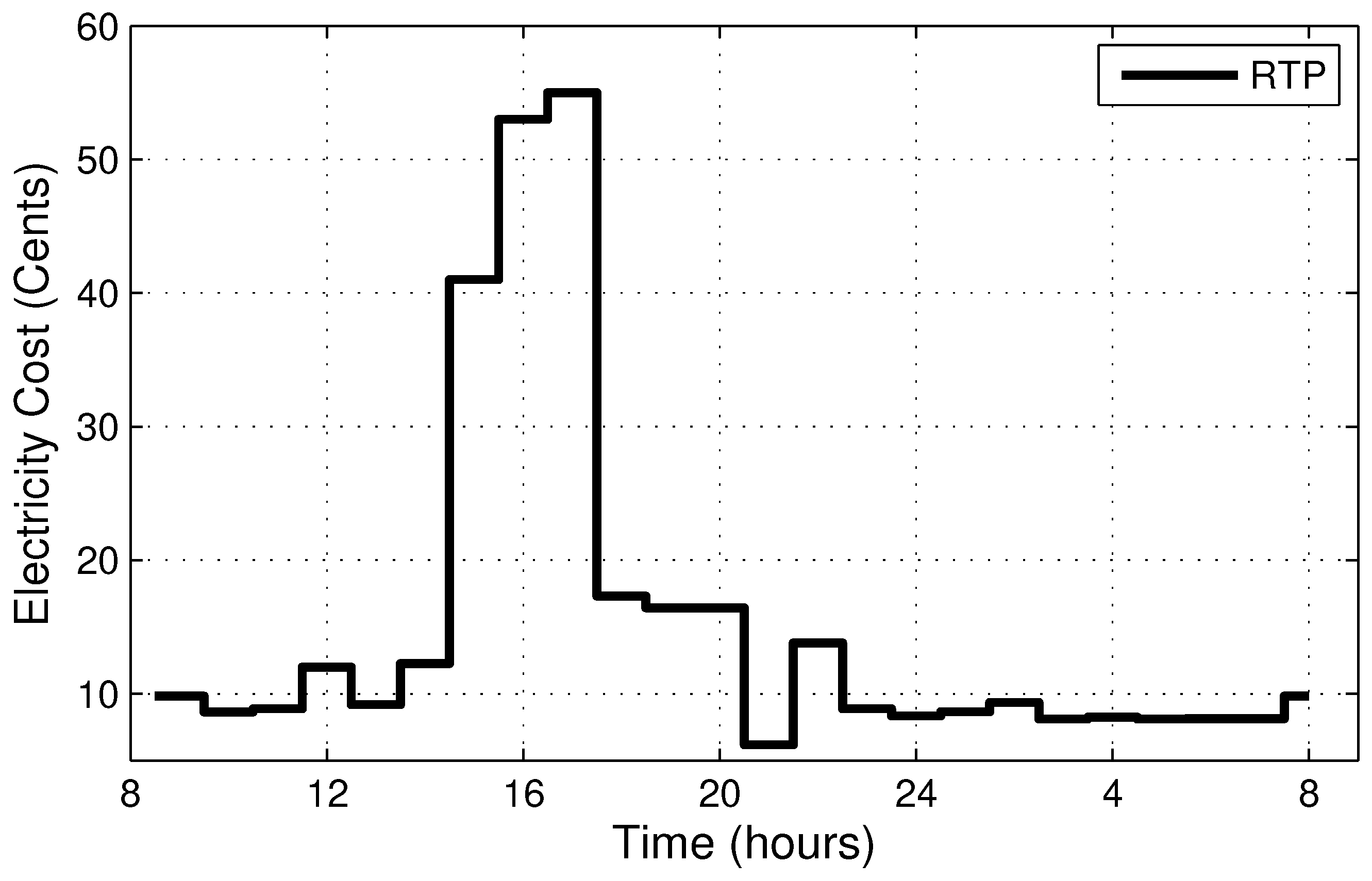
7.2. Pricing Signal
Different pricing signals were available. We used the day-ahead real time pricing (RTP) signal in our simulations, as shown in
Figure 5.
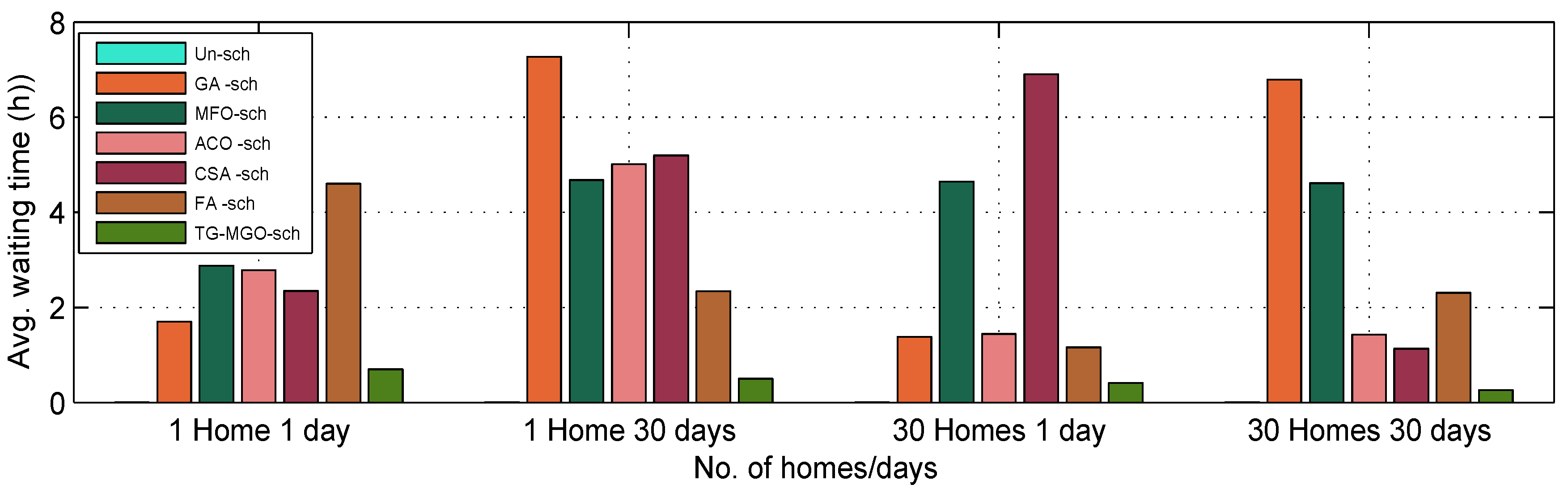
7.3. The Average Waiting Time
Waiting time is a very important feature of appliance scheduling for optimal energy consumption in the smart grid. To reduce electricity cost, usually, waiting time increases. A user wants to start an appliance, but due to scheduling time constraints, the user has to wait for to start its operation. Our main objective in this work was to minimize the user electricity bill, keeping in view the maximum comfort level of the end-user.
Figure 6 shows that we achieved our objective using heuristic techniques for optimal scheduling. The graphs show that TG-MFO outperformed ACO, CSA, GA, FA and MFO in achieving a nearly-zero waiting time for the end-user.
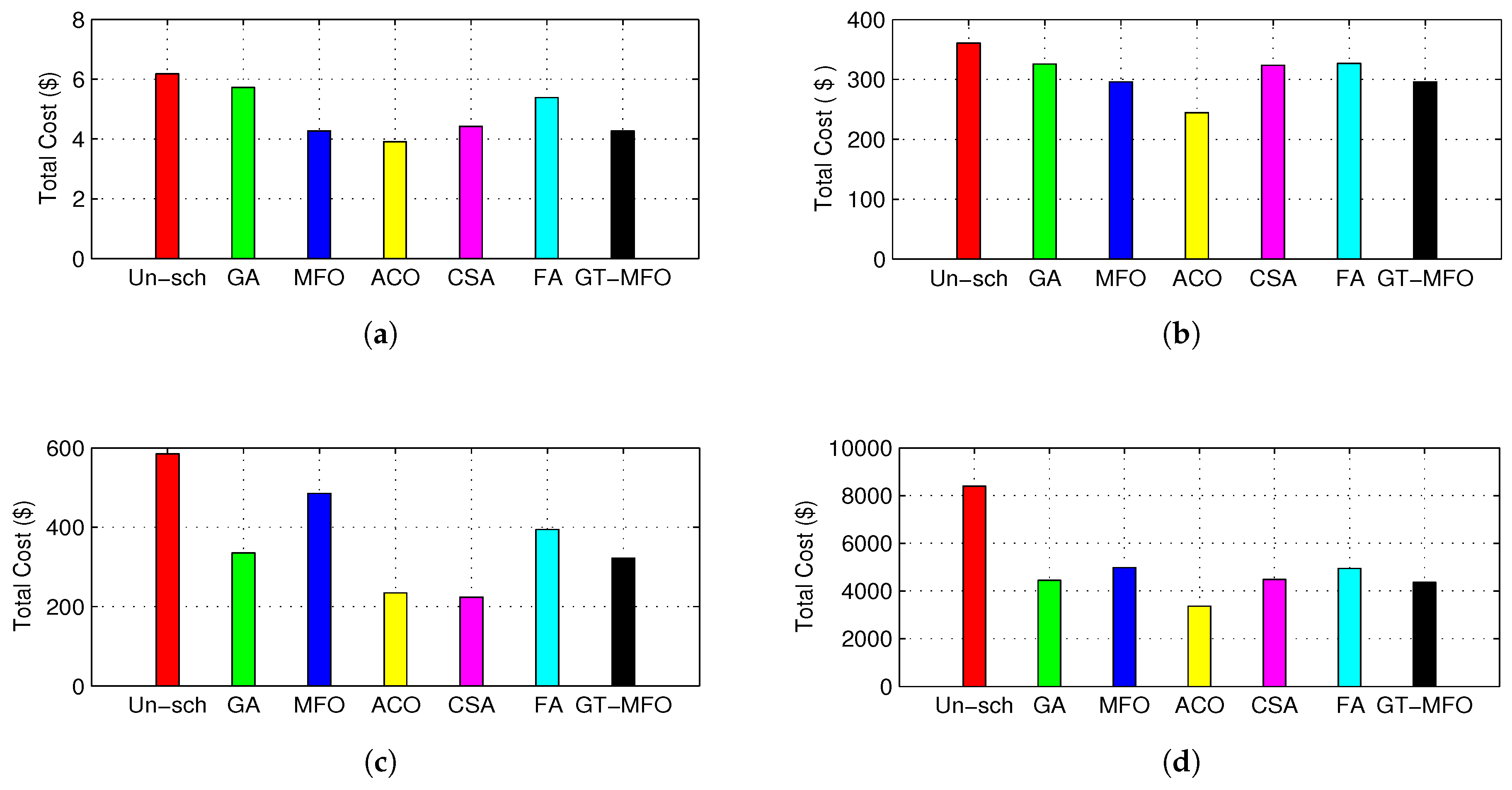
7.4. The Total Electricity Cost
Figure 7 shows the electricity cost for the unscheduled and scheduled (with ACO, CSA, GA, FA, MFO and TG-MFO) load. The results show that the electricity cost of the meta-heuristic algorithms-based scheduled load was very low as compared to the unscheduled load cost. In
Figure 7a, the operation of a single home for a single day is considered. In this case, ACO-based scheduling showed better results as compared to all scheduled and unscheduled costs. Similarly, in
Figure 7b, the case of a single home for 30 days (one month) is shown, in
Figure 7c, that of 30 homes with different LOTs and power ratings for 30 days (one month), and in
Figure 7d, the case of 30 homes for 30 days; the scheduled cost was very much as compared to the un-scheduled cost. In all four cases, ACO outperformed all scheduling techniques.
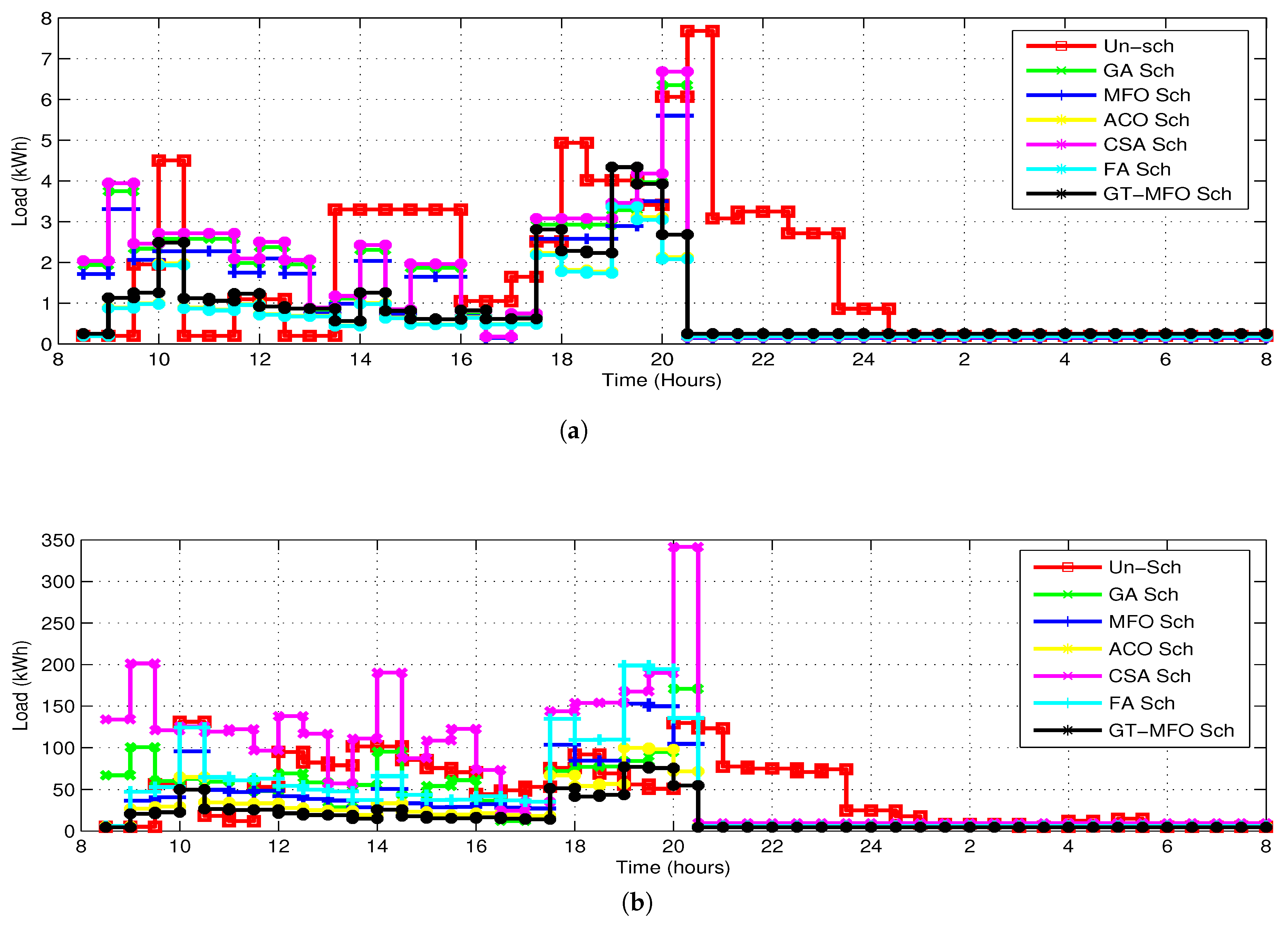
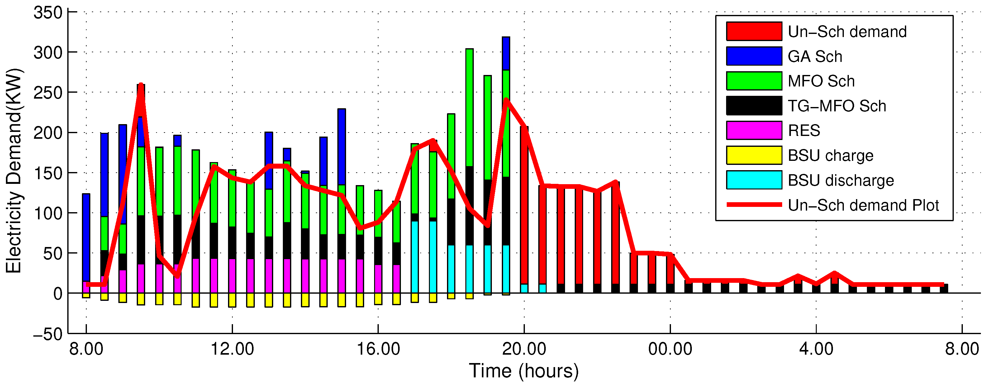
7.5. Hourly Load
Figure 8 shows the total hourly load of a single home and 30 homes with unscheduled and scheduled loads with the bio-inspired algorithms ACO, CSA, GA, FA, MFO and TG-MFO. The results show that as compared to the unscheduled load, meta-heuristic algorithm-based scheduled load was shifted to the off-peak hours, where not only the price was low, but RES was also available, considering the end-user’s time constraints for the maximum comfort level. The figure shows that our proposed algorithm gave comparative results for both single and multiple homes with different sizes, power ratings and LOTs.
7.6. Integration of RES and BSU
In order to minimize the consumed energy for further reduction of the total cost, RES and BSUs were integrated in homes.
Figure 9 shows that the day-time load will be supported by RES, while extra energy will be stored in BSUs for running the load in peak hours. It drastically reduced the cost. The figure depicts that our proposed TG-MFO algorithm has intelligently not only shifted the load to day-time off-peak hours for cost minimization, but also reduced the PAR.
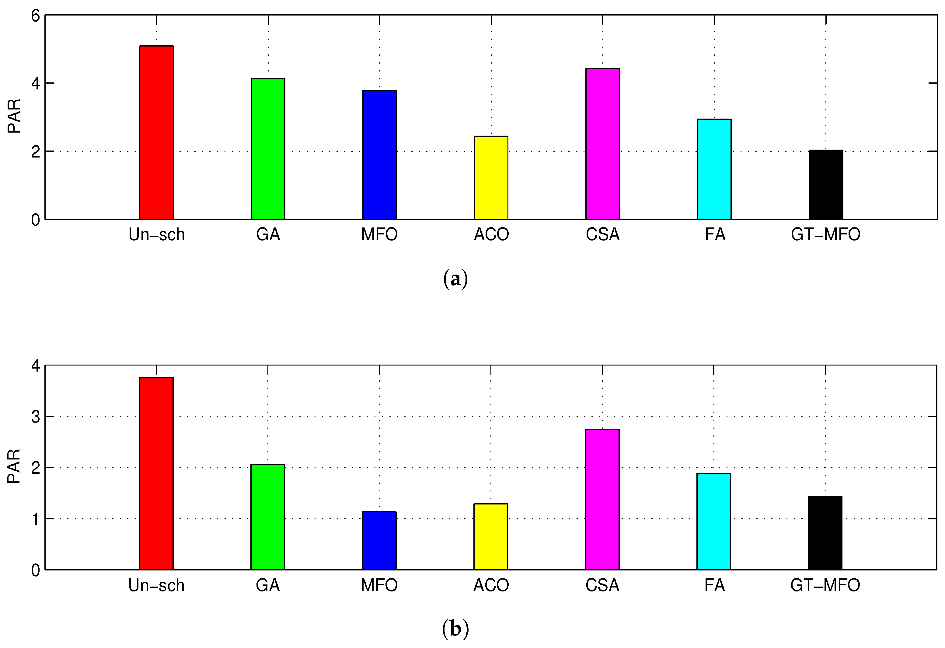
7.7. PAR
PAR plays an important role in the optimal scheduling of smart home appliances. Due to high PAR, the utility faces huge peak loads during peak hours, and the rest of the day, most of the generating units remain idle. Therefore, researchers try to reduce PAR for economical load dispatch in smart grids.
Figure 10 shows that, in the case of a single home for a single day and thirty homes for a single day, MFO performed better than FA, while in the case of a single home for thirty days and thirty homes for thirty days, FA showed better results than MFO. In our proposed hybrid model, we tried to not only schedule appliances optimally, economically and having maximum end-user comfort, but also gave the lowest PAR, for the benefit of utility, and hence, to further increase the end-user comfort level.
A comparison of the proposed algorithm with state-of-the-art research works in the smart grid environment for energy optimization and end-user comfort is depicted in
Table 8. Most of the existing techniques have used trade-offs between user comfort and bill minimization.
Table 9 shows the performance of the proposed TG-MFO algorithm, compared to unscheduled load and scheduled with the GA, MFO, ACO, FA and CSA algorithms.
Table 10 shows the runtime of the proposed algorithms using an Intel (R) Core (TM) i5 processor, with 4.00 GB of installed memory (RAM) and the 32-bit Windows 7 Operating system.
8. Conclusions and Future Work
In this paper, we mapped GA, MFO and a new efficient and robust hybrid TG-MFO meta-heuristic bio-inspired algorithm for optimal scheduling of home appliances in the smart grid and compared their results with existing techniques of CSA, FA and ACO. We considered a single- and multiple home scenarios in a residential sector. In multiple homes, we took different LOTs and power ratings of appliances to make it more practical. Day-ahead RTP signalling was used for demand response in smart homes. The results show that there was a 6.45%–49.03%, 32.26%–41.10% and 32.25%–49.96% decrease in the total cost with GA, MFO and TG-MFO scheduling, respectively, for single and multiple users. RESs and BSUs were also integrated to obtain a further decrease in the total cost and end-user waiting time. In this work, we tried to not only reduce the total cost, but to achieve a high comfort level of the end-user by minimizing the waiting time of home appliances using the time constraints of a maximum average delay of 0.26–0.62 h. This algorithm can be applied to actual data when and where they are provided. It not only reduces the energy cost, but also increases the stability and reliability of the grid. Future work includes exploration of more bio-inspired algorithms for intelligent and efficient energy optimization, and a multi-objective approach will be applied.


