Provision of Ancillary Services from an Aggregated Portfolio of Residential Heat Pumps on the Dutch Frequency Containment Reserve Market

Featured Application

Operating an aggregation of heat pumps for market-based provision of Frequency Containment Reserves.

Abstract

This study investigates the technical and financial potential of an aggregation of residential heat pumps to deliver demand response (DR) services to the Dutch Frequency Containment Reserve (FCR) market. To determine this potential, a quantitative model was developed to simulate a heat pump switching process. The model utilizes historical frequency and heat pump data as input to determine the optimal weekly bid size considering the regulations and fine regime of the FCR market. These regulations are set by the Dutch Transmission System Operator (TSO). Two strategies were defined that can be employed by an aggregator to select the optimal bid size; the ‘always available’ scenario and the ‘always reliable’ scenario. By using the availability and reliability as constraints in the model, the effects of TSO regulations on the potential for FCR are accurately assessed. Results show a significant difference in bid size and revenue of the strategies. In the ‘always available’ scenario, the average resultant bid size is 1.7 MW, resulting in €0.22 revenue per heat pump (0.5kW_p) per week. In the ‘always reliable’ scenario, the average resultant bid size is 7.9 MW, resulting in €1.00 revenue per heat pump per week on average in the period 03-10-2016–24-04-2017. This is based on a simulation of 20,000 heat pumps with a total capacity of 1 MWp. Results show a large difference in potential between the two strategies. Since the strategies are based on TSO-regulations and strategic choices by the aggregator, both seem to have a strong influence on the financial potential of FCR provision. In practice, this study informs organizations that provide FCR with knowledge about different bidding strategies and their market impact.

1. Introduction

With the transition towards a low-carbon energy supply system underway, the share of electricity generated by renewable energy resources (RER) is likely to increase. In Europe, wind and solar energy have the highest potential in terms of renewable electricity generation [1]. Wind and solar energy resources are intermittent, as their availability depends on weather patterns [2]. To maintain the system frequency within acceptable limits, electricity supply and demand needs to be balanced. Traditionally, supply could be adjusted to match demand by dispatching fossil-fueled generators. Given the transition towards renewable energy generation, the traditional electricity grid needs to be shifted towards the so-called smart grid notion, in which new technologies can be implemented without jeopardizing grid reliability and efficiency, and which make the grid less environmentally friendly [3]. A smart grid allows grid-elements which are only passively used in the current electricity system to become actively involved in the provision of system services such as balancing activities [4]. An important aspect of smart grids is Demand Response (DR). Also known as a category of the general term demand side management [5,6], Demand response is defined by [7] as ‘The process through which final consumers (households or businesses) provide flexibility to the electricity system by voluntarily changing their usual electricity consumption in reaction to price signals or to specific requests, while at the same time benefiting from doing so’.

In the deregulated energy market, a consumer that takes an active role in energy generation and/or provision of flexibility services is referred to as a prosumer [8,9]. For small consumers to become prosumers by using their flexible load for financial or balancing purposes, a new role is needed in the energy value chain: the role of aggregators. An aggregator is defined by [10] as ‘an intermediary between small consumers and other players (e.g., the retailers, or distribution companies) in the system’ (pp.138). Aggregators bundle the flexibility of individual consumers or businesses into a portfolio of devices that are either switched on or off, depending on grid stabilization requirements. In so doing, aggregators enable smaller system users (consumers or producers) to participate indirectly in the market through the provision of flexibility services, and to receive financial benefits in return. An example of this is Direct Load Control (DLC), in which the aggregator directly controls a set of appliances within the end-user’s premises [11].

Recent developments in the energy market liberalization process have created several opportunities for aggregators for the provision of market-based products and services [12]. In the Netherlands, short-term frequency deviations are balanced through the Frequency Containment Reserve (FCR) market, also known as primary reserve [13]. In the FCR market, a bidding system is applied in which parties offer a certain amount of flexible power that they can deliver whenever necessary. In return, they receive financial compensation from the Transmission System Operator (TSO) for the capacity they have offered. Given that FCR is important to system reliability, it must be provided continuously, with an availability of 100% [14]. Not meeting the promised bid results in a fine, which the DR-aggregator must pay to the TSO.

Aggregators need to construct their flexible portfolio of DR assets in such a way that it delivers the promised amount of flexibility while meeting the prerequisites of the FCR market. With a given portfolio, aggregators can choose how much flexibility they are willing to provide during the next bidding period. Determining the bid size for each bidding period is a strategic process. If the aggregator bids too low, revenue, and thus profit, can be suboptimal. On the other hand, if the aggregator bids too high, the aggregator might be unable to deliver the flexibility, and thus risks a fine. The length of the bidding period is country- and market-specific. When the bid size is determined, the aggregator is bound to deliver that amount of flexibility during the complete bidding period, in response to frequency deviations [13].

Many different technologies have the potential to operate as DR-assets, in the residential, commercial and industrial sectors. An example is the residential heat pump. Heat pumps convert electrical power into heat, used for heating households and supplying hot tap water, and thus, have a fundamental role in efficient energy use in residential buildings [15]. Heat pumps show large potential in abating CO₂ emissions, and this is accelerated by increasing shares of renewable electricity generation [16,17]. In contrast to gas-fired boilers, heat pumps are most efficient when operating at low temperatures, and are therefore considered slow response heating systems [18]. This may be a positive aspect from the perspective of switching them on or off in a DR event. Even though it is widely recognized that heat pumps can be used as flexibility assets in DR-portfolios, their flexibility is currently only rarely utilized [19].

Most research conducted in this field of study focusses on the technical performance of heat pumps in providing flexibility [20,21,22]. However, no literature studies were found that investigate aggregator bidding process optimization strategies. Also, the potential financial revenues resulting from offering flexibility on the Dutch FCR market using these strategies seem largely unknown. Therefore, the scientific contribution of this work lies in:

• Insights into the effects of potential aggregator bidding strategies that on the potential of FCR
• An assessment of the economic potential of domestic heat pumps to deliver flexibility on the FCR market. This potential is measured in revenue per household
• The development of a quantitative model to assess the potential of FCR, and an explanation of the model logic
• A detailed assessment of the effects of TSO-regulation on the potential for FCR

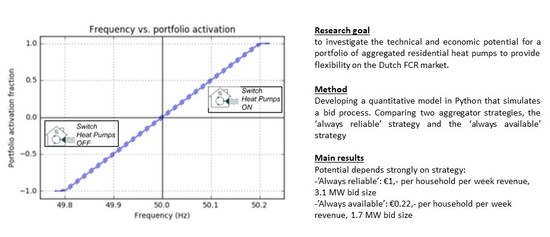
This study aims to investigate the technical and economic potential for a portfolio of aggregated residential heat pumps to provide flexibility on the Dutch FCR market. Economic potential is measured by revenue generated from providing FCR, whereas technical potential is measured in terms of bid capacity given technical constraints. In addition to the technical and economic potential, the effect of fine regulations, i.e., fines for non-availability and inadequate response, is thoroughly investigated.

Two strategies are considered that the aggregator can apply to determine the weekly bid size: the ‘always available’ strategy and the ‘always reliable’ strategy, both based on availability and/or reliability. Both strategies, as well as the concepts of reliability and availability, are explained in the method. In addition, an explanation is provided of how the model functions and how the results can be interpreted.

The paper is structured as follows. The methodology section starts with an explanation of the TSO-regulations, bidding strategies and model details. Information is then provided regarding data processing and frequency analysis, followed by a detailed explanation and overview of the model functionalities. The results section begins with the general model results. This is followed by an analysis of reliability, availability and monetary flows, and an analysis of grid frequency. After the discussion and conclusion section, the appendix provides more details regarding the TSO fine regime and household availability.

2. Method

2.1. TenneT Fine Regime and Product Specifications

DR is limited by three regulatory factors: minimum bid size, minimum bid duration and binding upward and downward bids [23]. The most important specifications for the Dutch FCR market are described in

Table 1. FCR product specifications [24]

Specification	Description	Value & Unit
Bidding period	The length of the period over which a bid is placed. During this period, the bidding party must always be able to deliver the amount of flexibility that has been bid.	Weekly
Minimum bid size	The minimum bidding capacity. Bids with lower capacities are not processed.	1 MW
FCR full-activation time	Within this time frame, the portfolio must be fully activated (100% capacity). Due to the 5-min resolution of the data, the full activation time is not taken into account in this study.	30 s
Insensitivity range	The range of frequency deviation to which the response of the system is insensitive.	10 mHz
Full activation deviation	The maximum frequency deviation to which the system must respond with full capacity.	100 mHz

based on a document describing the product specifications.

In cases where the aggregator is not available or not able to respond adequately, the aggregator will be fined by the TSO. Two types of fines are enforced in the Dutch FCR-market: fines for non-availability (NA-fines) and fines for inadequate response (IR-fines) [25]. NA-fines are imposed when the available flexible power is lower than the bid capacity. Hence, this fine can also be imposed when this flexible power is not requested by the Distribution System Operator (DSO). In contrast, IR-fines are only imposed when the aggregator does not respond adequately to a given frequency deviation. A description of both fine regimes is provided in Appendix A—TenneT TSO Fine Regime, as specified in a framework agreement concerning primary reserve [13].

2.2. Bidding Strategies

In this study, two different strategies are considered for determining how much capacity to bid on the FCR market, i.e., the ‘always reliable’ strategy, and the ‘always available’ strategy. The ‘always available’ strategy aims for perfect performance. It does so by determining bid size in such a way that with a given portfolio consumption, the aggregator is always able to deliver 100% of the bid capacity in both directions, at any frequency deviation. In so doing, the aggregator risks neither NA-, nor IR-fines. The ‘always reliable’ strategy aims to deliver 100% service reliability by choosing a bid size in which the portfolio has sufficient capacity to respond to the historical frequency deviations that are used as input for the model. This strategy does not result in any IR-fines, since given the determined bid size, the aggregator is able to respond to the historical frequency deviations. However, unlike the ‘always available’ strategy, this strategy will lead to NA-fines, since the aggregator is not always able to respond correctly to a 100% frequency deviation. The ‘always reliable’ strategy can be considered a low-risk strategy compared to the ‘always available’ strategy, since the chosen bid size, and therefore, the revenue, is expected to be lower.

2.3. Model Details

For this study, a quantitative model has been developed in Python (V3.5.2, Anaconda version 4.2.0, 2016,) in which historical frequency and heat pump data are used to simulate a bid process. Data from 33 households is used and scaled up to represent a portfolio of 20,000 heat pumps of 10 MW aggregated capacity with time-steps of 5 min Based on historical frequency measurements, the required amount of flexibility for every 5-min interval was determined. By simulating the switching of the heat pumps, the revenue and the fines were calculated for an iteratively increasing bid size. This process was performed for every week, leading to weekly revenue, availability percentage and reliability percentage.

2.4. Data Selection and Frequency Analysis

The data used for this study comes from Energiekoplopers, a Dutch Pilot project in Heerhugowaard aimed at assessing the potential of flexibility in residential energy systems [26]. The total dataset that was available for this study consisted of 33 households containing a heat pump. The heat pumps used were air-sourced heat pumps from the brand Inventum Ecolution Combi 50. Their minimum electrical capacity was 5W and their maximum was 500W. From these heat pumps, data presenting the power demand for the heat pump per 5 min was used for a period of 30 weeks, between 01-09-2016 and 01-05-2017. No data was available from the end of December until the beginning of February. As a result of this missing data, an 8-week gap occurs in this period, leaving 22 weeks of useful data (see Appendix B—Number of households per week).

Due to measurement errors during the pilot demonstration project, several data gaps occur in the dataset and the start date and end date between when data is available varies strongly per household. Since the bidding period as defined by TenneT is a week, the dataset was split into datafiles of one week. Data points containing extreme outliers were excluded. In addition, when more than 60 consecutive min. of heat pump data were missing, the data of that week were deleted for that heat pump. These research choices resulted in a relatively small, but reliable dataset. In order to obtain a viable portfolio size of 10 MW, the number of households was scaled up to 20,000 for every week.

2.5. Determining Availability, Reliability and NA-fines

To calculate the NA-fines for every bid size, upper and lower boundaries were determined. The upper boundary was calculated by subtracting the bid size from the maximum possible power consumption, whereas the lower boundary is calculated by adding the bid size to the minimum possible power consumption. When the power consumption exceeds those boundaries, the portfolio is not able to deliver 100% flexibility in that direction, resulting in a fine that follows the fine regime (Section 2.1) used in this study. The availability is then calculated as the number of NA-events divided by the amount of data points per week, which is 2016 5-min timestamps.

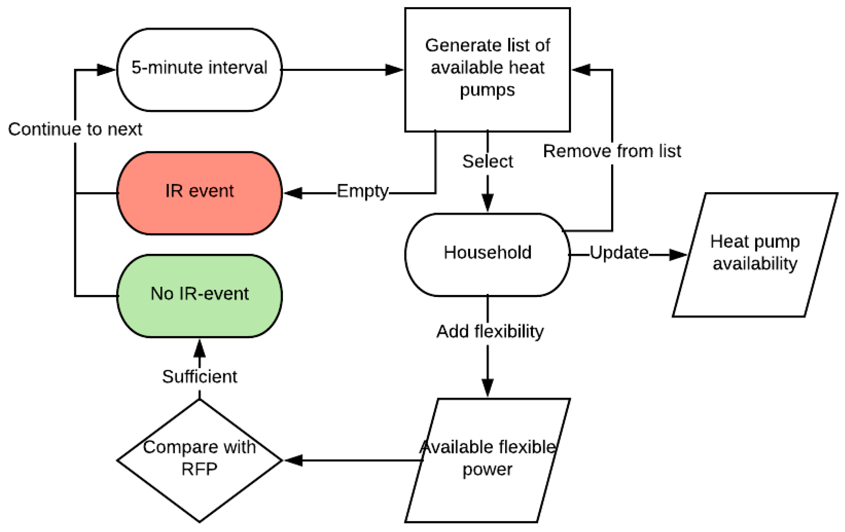
To determine reliability at a given bid size, an assessment of whether the portfolio was able to respond correctly needs to be made for every timestamp in the model. In this study, the required portfolio response is expressed in terms of Required Flexible Power (RFP). This describes the power that the portfolio should shift at each moment. A negative RFP represents a downward shift and a positive RFP represents an upwards shift to the baseline. When the portfolio is not able to deliver the RFP, a so called ‘IR-event’ occurs. The reliability can then be calculated as the percentage of timestamps in which no IR-event occurred.

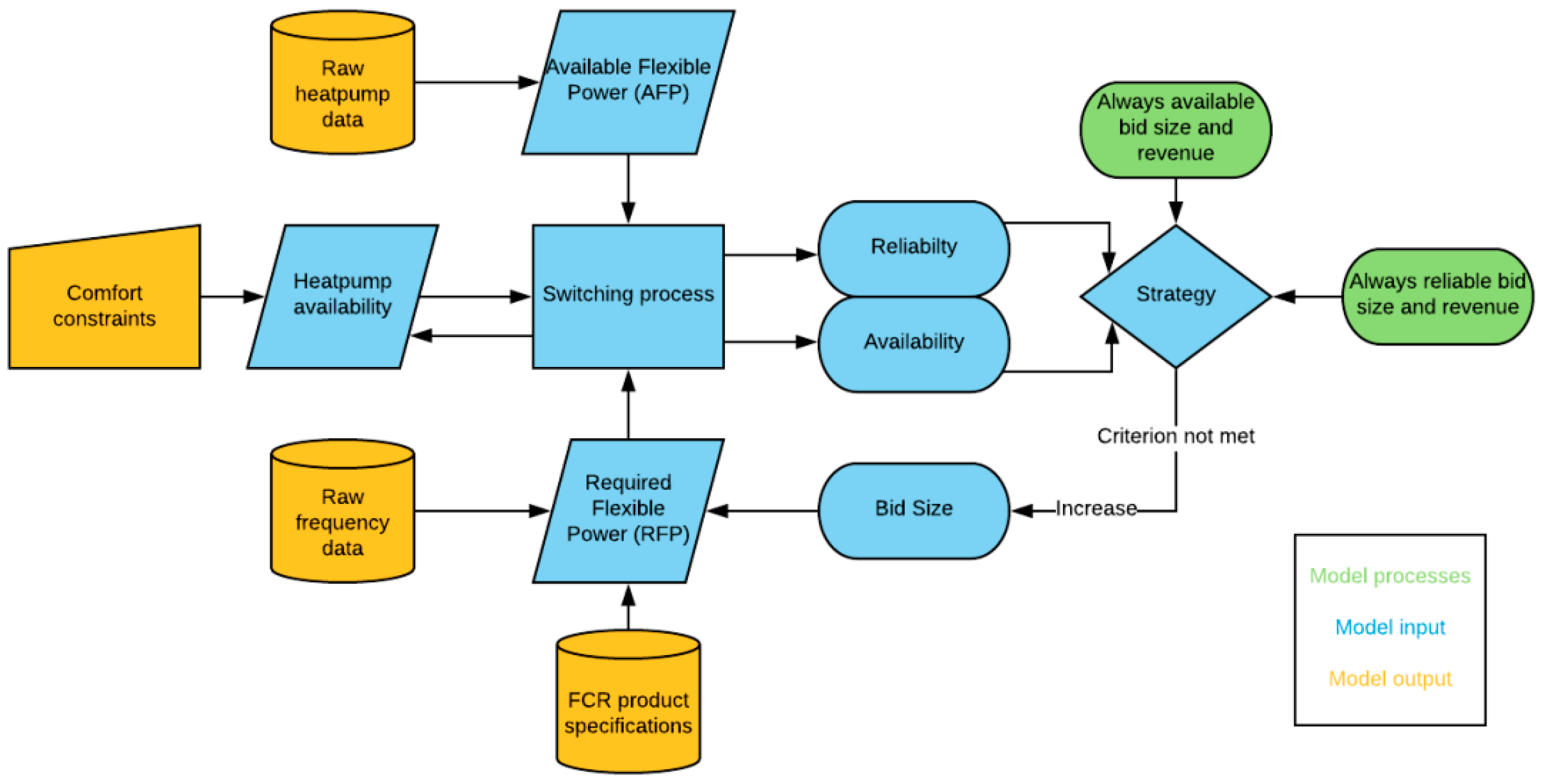
Determining whether an IR-event occurs is a repetitive process performed in multiple steps. First, a list of available households is generated, and a household is selected from that list. Then, a household is taken from that list and the Available Flexible Power (AFP) of that household is added to the Total Available Flexible Power (TAFP), after which the household is removed from the list and the availability is updated. This process is repeated until either the list of available households is empty, or the TAFP exceeds the RFP. If the list of available households is empty before the TAFP exceeds the RFP, then an IR-event occurs. If not, then no IR-event occurs. In both cases, the model breaks out of the loop and continues to the next 5-min interval. In Figure 1, this process is illustrated.

The RFP can be calculated by dividing the frequency deviation (F_actual – F_target) by the Full Activation Deviation (FAD) and multiplying it with the bid size:

$$RFP\left(t\right)=Bidsize\ast \frac{F_{actual}-F_{target}}{FAD}$$

(1)

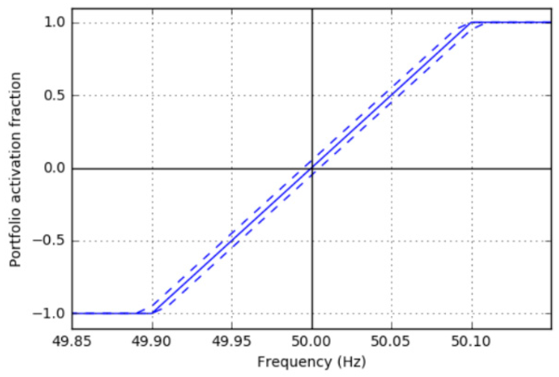
Since no more than 100% flexibility is required, the RFP cannot exceed (positively or negative) the bid size. The upper and lower boundaries of the RFP can be calculated by adding or subtracting the insensitivity range to the actual frequency (F_actual). In Figure 2, the portfolio activation fraction is displayed, representing the percentage of the portfolio that should be activated at any given frequency. This method is applied for every frequency measurement in the model to calculate the RFP.

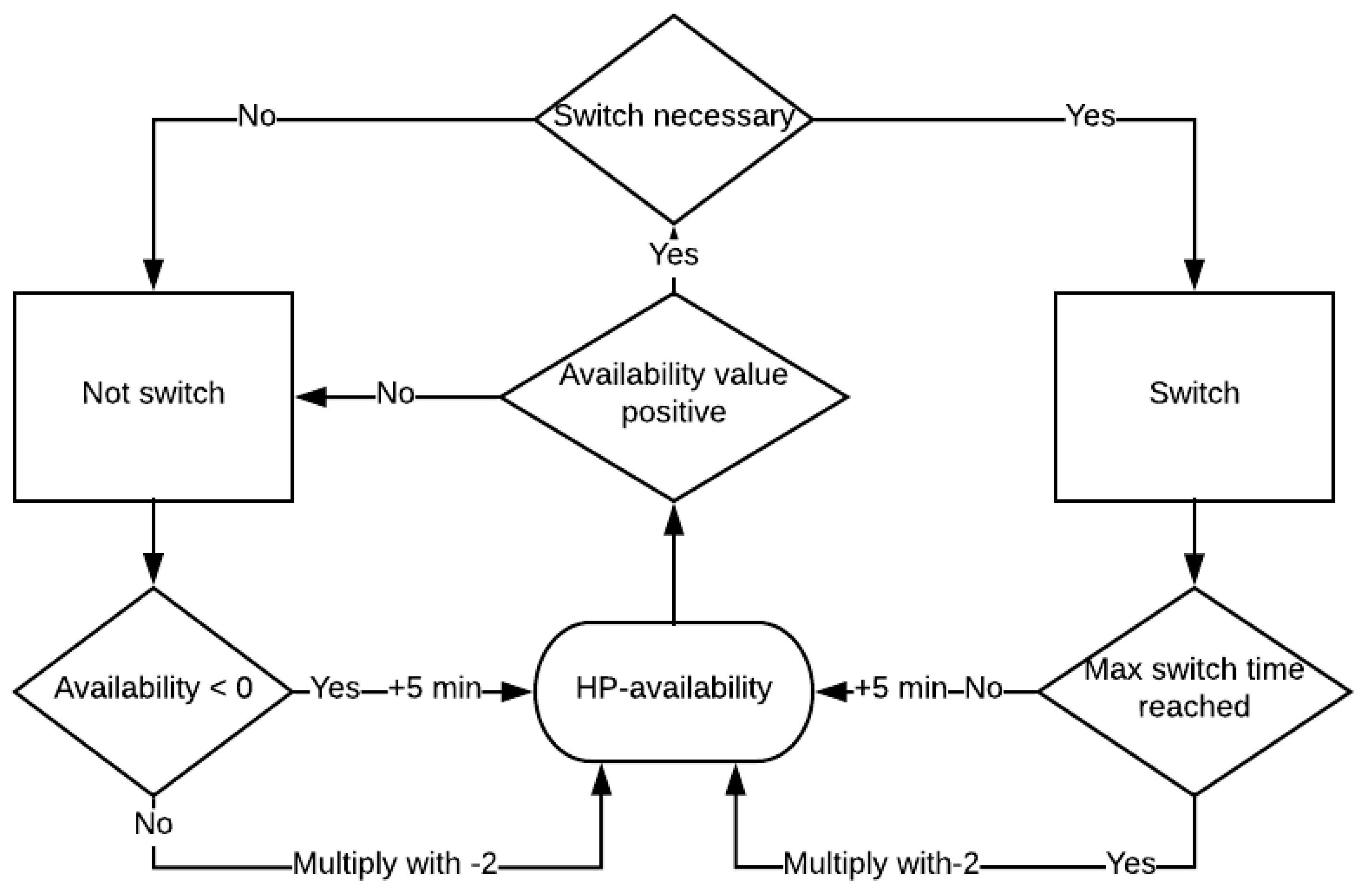
The main drawback of using heat pumps for DR-purposes lies in the constraints of the end-users that require a room temperature that is comfortable to live in [27]. In the model, this constraint is implemented in a simplified way by implementing a maximum switch time, thereby limiting the time that the heat pumps can be switched for. To enforce this principle, an availability-module is implemented into the model that limits the heat pump’s availability for switching to a maximum of 15 min at a time. In this module, the availability status of every heat pump is stored. Heat pump availability in both directions will be stored in a data frame. The availability module works with a value for availability that is checked and updated for every 5-min interval in the model.

When the heat pump is switched, 5 min are added to the (positive) value of heat pump availability for that household at that moment. When the heat pump is not switched while it is non-active (availability < 0), 5 min are added to the availability, making it less negative. When the availability changes from −5 to 0, the heat pump will be available for switching again. Only heat pumps with a value of availability that is equal to 0 or positive can be switched. This process is illustrated in Figure 3.

To select heat pumps that should be switched first, heat pumps are divided in two categories:

• Heat pumps with HP-availability > 0: these were switched in the previous timestamp but are still available. Switching these heat pumps first is most efficient.
• Heat pumps with HP-availability = 0: these are available and were not switched in the previous timestamp. These should be switched when no category 1 heat pumps are available.

To find the heat pump that should be switched, the model first iterates over the category 1 heat pumps. If no available heat pumps exist within this group, the model will start iterating over the category 2 heat pumps. Within both groups, the algorithm looks for the heat pump that has the highest contribution of flexibility related to the RFP. It calculates the absolute difference between AFP and RFP for every heat pump. The heat pump with the highest flexibility potential will be selected as the heat pump to be switched.

2.6. Determining Bid Size and Associated/Potential Revenues

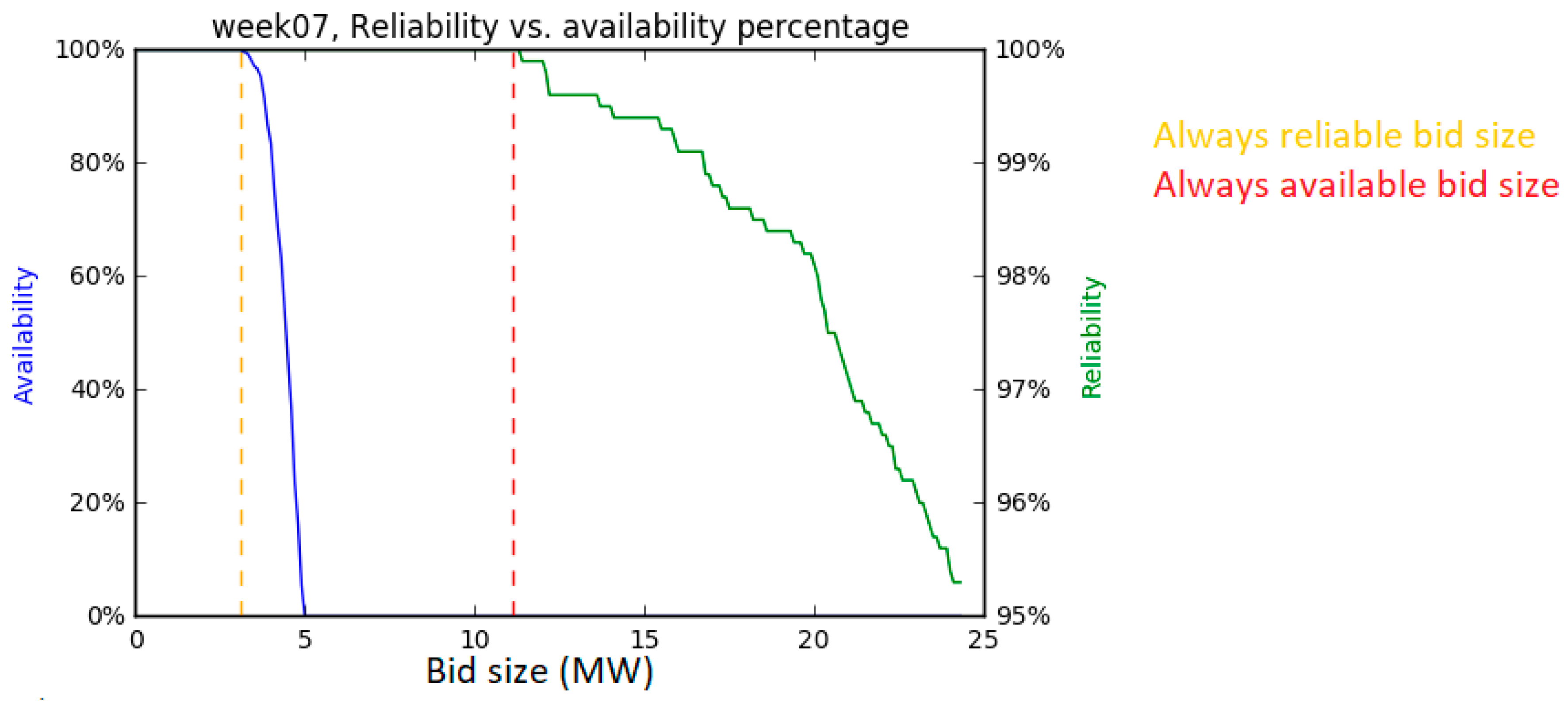
To obtain the bid size and revenue for both strategies, the model iterates over an increasing bid size, obtaining the reliability and availability for each iteration. When the reliability drops below 100%, the ‘always reliable’ bid size is selected as the bid size in the previous iteration. The ‘always available’ strategy bid size is determined in the same manner. For the main results, the bid size is increased in steps of 100 kW, starting with a minimum bid size of 100 kW. A relatively small bid size step provides high accuracy, resulting in smooth graphs and accurate results.

The revenue is based on the FCR price, expressed in €/MW/week. These prices are received from ENTSO-E (2018) and differ per week. They are based on the highest bid price in the given period. Therefore, in this study, it is assumed that the bid price equals the FCR price. In the period that is relevant for this study, prices range from €1936.77/MW/week to €3354.80/MW/week, with an average of €2559.49/MW/week. The revenue per week can be calculated by:

$$Revenu{e}_{week\left(x\right)}=Bidsize\ast FCRprice$$

(2)

2.7. Model Overview

In Figure 4, a visualization of the model is presented. The input for the model consists of the raw heat pump data, the raw frequency data, FCR product specifications and comfort constraints of the households. This input forms the basis for the AFP, RFP and heat pump availability, which are used for the switching process. When the switching process is repeated for every 5-min interval in the model, the availability and reliability are determined for the given bid size. The model starts with a low bid size, while iteratively increasing it until both the reliability and availability drop below 100%. The bid size at which the availability first drops below 100% was the bid size for the ‘always available’ strategy, whereas the bid size at which the reliability first drops below 100% was the bid size for the ‘always reliable’ strategy. Both revenues can be calculated based on the bid size.

3. Results

3.1. General Results, a Comparison between both Strategies

By using the ‘always available’ strategy, the aggregator successfully aims for a bid size that results in zero fines. As a result, both the availability percentage as well as the reliability are 100%. This strategy yields a lower bid size and revenue compared to the ‘always reliable’ strategy. With this strategy, a total of €96,114 can be earned, with an average bid size of 1.7 MW. With the ‘always reliable’ strategy, the total revenue is €438,318 with an average bid size of 7.9 MW. However, even though the aggregator was able to respond correctly to given frequency deviations, the low availability of only 9% that results from this strategy leads to €2,220,398 fines for non-availability. In

Table 2. Results for the ‘always available’ strategy.

	Bid Size (MW)	Revenue (€/week)	Revenue/Household (€/week/household)	Availability (%)	NA-Fines (€/week)
week01	0.3	€648,-	€0.03	100%	€-
week02	1.0	€2190,-	€0.11	100%	€-
week03	1.0	€2350,-	€0.12	100%	€-
week04	1.7	€4148,-	€0.21	100%	€-
week05	1.5	€3840,-	€0.19	100%	€-
week06	2.9	€6960,-	€0.35	100%	€-
week07	3.1	€7192,-	€0.36	100%	€-
week08	2.9	€6873,-	€0.34	100%	€-
week09	3.0	€7170,-	€0.36	100%	€-
week10	3.0	€7380,-	€0.37	100%	€-
week11	2.6	€6266,-	€0.31	100%	€-
week20	2.9	€8410,-	€0.42	100%	€-
week21	1.6	€5136,-	€0.26	100%	€-
week22	1.4	€4340,-	€0.22	100%	€-
week23	1.1	€3300,-	€0.17	100%	€-
week24	1.3	€3718,-	€0.19	100%	€-
week25	2.0	€5320,-	€0.27	100%	€-
week26	0.4	€964,-	€0.05	100%	€-
week27	0.8	€1760,-	€0.09	100%	€-
week28	1.4	€2954,-	€0.15	100%	€-
week29	2.3	€4968,-	€0.25	100%	€-
week30	0.1	€227,-	€0.01	100%	€-
Average	1.7	€4368,-	€0.22	100%	€-
Total	N/A	€96,114,-	€4.81	N/A	€-

and

Table 3. Results for the ‘always reliable’ strategy.

	Bid Size (MW)	Revenue (€/week)	Revenue/Household (€/household/week)	Availability (%)	NA-fines (€/week)
week01	1.8	€3888,-	€0.19	61%	€5025,-
week02	5.7	€12,483,-	€0.62	0%	€41,921,-
week03	5.8	€13,630,-	€0.68	0%	€59,075,-
week04	8.8	€21,472,-	€1.07	0%	€120,521,-
week05	7.0	€17,920,-	€0.90	0%	€81,932,-
week06	11.2	€26,880,-	€1.34	0%	€163,223,-
week07	11.3	€26,216,-	€1.31	0%	€160,418,-
week08	11.6	€27,492,-	€1.37	0%	€170,114,-
week09	10.4	€24,856,-	€1.24	0%	€142,704,-
week10	11.2	€27,552,-	€1.38	0%	€167,152,-
week11	8.5	€20,485,-	€1.02	0%	€99,575,-
week20	11.9	€34,510,-	€1.73	0%	€216,253,-
week21	9.8	€31,458,-	€1.57	0%	€179,374,-
week22	10.1	€31,310,-	€1.57	0%	€183,240,-
week23	4.9	€14,700,-	€0.74	5%	€14,330,-
week24	7.3	€20,878,-	€1.04	0%	€90,664,-
week25	7.0	€18,620,-	€0.93	0%	€81,174,-
week26	3.7	€8917,-	€0.45	36%	€16,668,-
week27	3.1	€6820,-	€0.34	53%	€8252,-
week28	8.2	€17,302,-	€0.87	0%	€91,692,-
week29	9.8	€21,168,-	€1.06	0%	€118,667,-
week30	4.3	€9761,-	€0.49	46%	€8423,-
Average	7.9	€19,923,-	€1.00	9%	€100,927,-
Total	N/A	€438,318,-	€21.92	N/A	€2,220,399,-

, an overview is presented of the main results for both strategies.

3.2. Reliability and Availability, Monetary Flows and upper and lower Boundaries to Power Consumption

The upper and lower boundaries are calculated by the methods explained in Section 2.5. When the upper and lower boundaries are exceeded by the power consumption, NA-fines occur, since the portfolio is not able to deliver the capacity required according to the corresponding bid size. This does not happen, since the bid size is chosen so that no fines will occur, leading to an availability of 100% with the ‘always reliable’ strategy. This is illustrated in Figure 5. The reliable bid size is therefore limited by the most extreme (upper or lower) values of the power consumption.

When the bid size exceeds half the portfolio capacity (5 MW), the lower boundary will become larger than the upper boundary, making it impossible for the portfolio to remain between the boundaries and deliver the required flexibility. In these cases, the availability drops to 0%, which results in NA-fines for every measurement. Since the boundaries resulting from the ‘always available’ strategy are extreme, they are not displayed in Figure 5.

Portfolio-availability represents the proportion of the week in which 100% flexibility can be delivered with the portfolio, whereas the reliability represents the fraction of the week in which the portfolio responded correctly given the frequency and corresponding RFP. The major difference between portfolio availability and reliability is that the reliability is strongly influenced by the frequency and RFP, whereas the portfolio availability is solely dependent on the power consumption of the portfolio and the bid size.

Figure 6 shows a steep decrease in availability, dropping from 100% availability at a reliable bid size of 3.1 MW to 0% availability at a bid size of 5.0 MW. Availability reduction to 0% at a bid size of 5.0 MW is explained by the fact that the portfolio will not be able to deliver 100% flexibility on a symmetrical market when the bid size exceeds half the maximum capacity. Therefore, in the model, the availability is always reduced to 0% when the bid size exceeds 5.0 MW. In contrast to the availability, the reliability will not drop to 0%. Even at extremely high bid sizes, when the frequency is 50 Hz, zero flexibility is required, and the portfolio is still able to respond correctly. This frequency-dependency is the main reason that the reliability shows a less-steep decline compared to the availability. Prevalence of frequency deviation occurrence is discussed in Section 3.3.

3.3. Frequency Analysis

In

Table 4. Average and max frequency deviations.

Resampling Method	Average Deviation	Max. Deviation	Average Portfolio Activation	Max Portfolio Activation
Original	17 mHz	140 mHz	8.5%	70.0%
Actual	16 mHz	110 mHz	8.0%	55.0%

, the average and maximum deviation and portfolio percentage are displayed for the original dataset and for the dataset resulting from the so-called ‘actual resampling method’. Using the actual resampling method has a diminishing effect on the average and maximum deviation, and thus, on the portfolio activation percentage. Given the small change in average deviation relative to the original dataset, the effect of the actual resampling method on the main results is considered minimal.

Figure 7 shows two plots, displaying the frequency distribution (top), and a distribution of the frequency deviation (bottom). In both cases, stronger deviations are less frequent compared to small deviations. This effect is visible to a larger extent in the mean dataset than in the original dataset. Frequency deviations of 0.1 Hz, in which 50% of the portfolio needs to be activated, seldom occur.

4. Discussion

Results show that availability is a stronger limiting factor to bid size and revenue than reliability. To make this effect visible, an ‘always reliable’ strategy was implemented, in which 100% availability was not a prerequisite. With this strategy, NA-fines were calculated, but did not affect the bid size and revenue. The NA-fines were displayed to give insights into the fines that would result if the aggregator would apply this strategy. Given the high risk of fines, the ‘always reliable’ strategy does not seem realistic to apply in practice. However, implementing it in the model shows that it is difficult for the TSO to apply NA-fines in practice. For the ‘always reliable’ strategy to be implemented successfully, a perfect knowledge about frequency deviations is required. In practice, prediction algorithms might make a rough estimation of the frequency deviations, but perfect knowledge about the frequency deviations one week in advance is not feasible. Therefore, selecting a bid size with the ‘always reliable’ strategy is merely a theoretical concept.

An important factor when switching heating systems for DR is that the comfort of households should not be jeopardized. Ideally, the effect of heat pump switching on household temperature should be included in the model by simulating household temperature. However, the dataset lacked the information required to perform this kind of analysis. Therefore, instead of temperature boundaries, a limit was set in this model on the length of time that heat pumps could be continuously switched. This limit was set to 15 min, after which a period of non-availability was implemented. During this period, the power consumption of the heat pump follows the baseline, as it would without any interference of a third-party aggregator.

An important factor for discussion in this study is the low data quality and availability resulting in many gaps and periods with irregular values. According to the method described, these gaps and constant values were either filled or filtered out, resulting in a small but reliable sample of data. Part of the data was excluded, decreasing the amount of viable data. Eight weeks of data were missing in December and January, usually the coldest months with the highest heating potential, which might lead to a slight underestimation of the potential for FCR. To correct for the small sample size, the portfolio of households has been scaled up to mimic a larger portfolio. By doing so, data has been duplicated to generate a 10 MW portfolio. This process might influence the results of this study, since these duplication methods lead to multiple heat pumps with the same fluctuation. In practice, 20,000 heat pumps, each with a unique baseline, will generate a more stable baseline when combined. With the frequency data, these problems did not occur. Certain research design choices were implemented to provide a reliable but rather conservative estimation of the economic and technical potential of residential heat pumps in the Dutch FCR market. This was due to the implications of the data availability and quality originating from this early pilot demonstration project. The main contribution of this paper is the proposed framework and the method and logic behind the model, which can be replicated for similar studies.

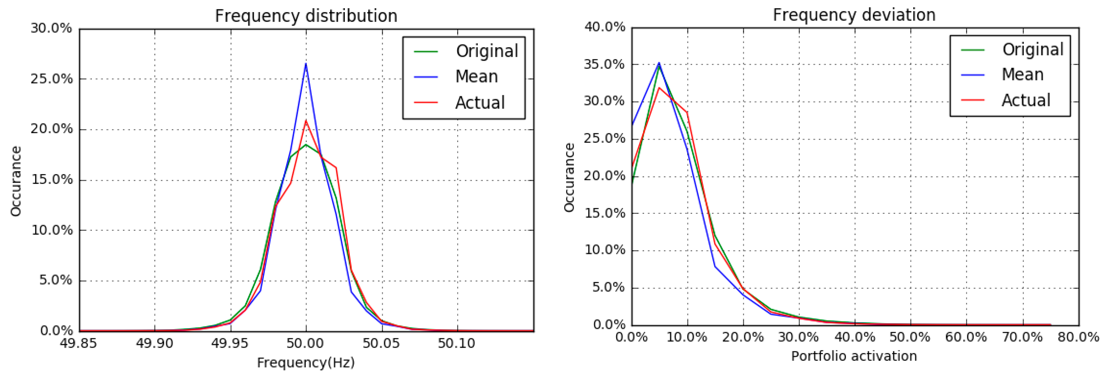
Another factor that may influence the outcome of this study is the resolution of the dataset. The household data was provided on a 5-min basis, whereas the frequency data was provided on a 10-second basis. In order to reduce the complexity of the model, the 5-min resolution was used as the model resolution. The frequency data was therefore down sampled from 10 s. to 5 min by using the methods described in Section 2.4

As a consequence, short term frequency deviations (within a 5-min time framework) could not be taken into account. For this reason, the FCR specification of 30 s response time could not be taken into account either.

TSO-regulation on what is considered an IR-event or NA-event is ambiguous. Therefore, in this research, an IR-event is defined as one 5-min interval in which the aggregator was unable to respond correctly. An NA-event is defined as one 5-min interval in which the portfolio has insufficient capacity to respond to an extreme (100% portfolio activation) deviation. In addition, the model holds the assumption that an IR-event or NA-event will lead to a fine in all cases. In practice, this might not be the case, since TSOs do not have the capacity to assess and verify every IR- or NA-event and respond accurately according to the fine regime. With an increasing participation of decentralized small assets in ancillary services markets, it would require automated verification methods to support the financial settlement. To obtain more accurate results, more specific information regarding TSO-regulation is required, as well as a higher resolution and quality of the dataset.

5. Conclusions and Recommendations for Further Research

5.1. Conclusions

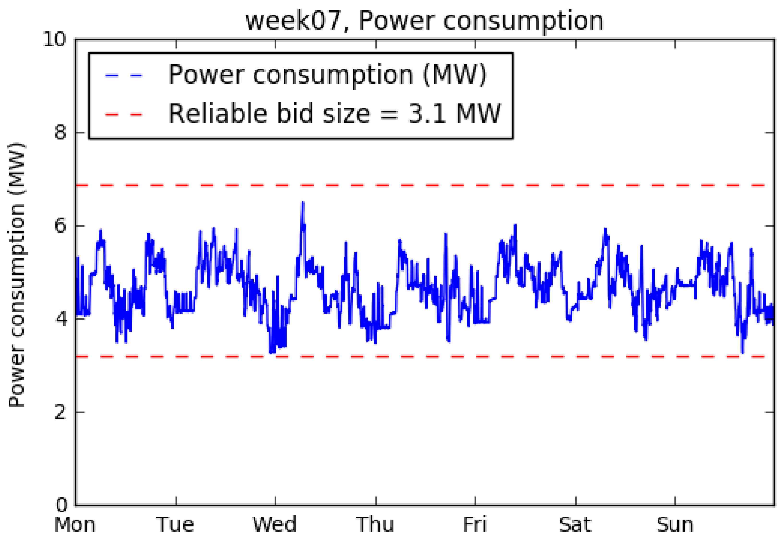
The main research question concerned the technical potential, and the economic potential of heat pumps to deliver ancillary services in the Dutch FCR market. The results show that both the technical and economic potential depend strongly on the bid strategy; the revenue resulting from this study is €0.22 per household per week in the ‘always available’ strategy, versus €1.00 per household per week in the ‘always reliable’ strategy. Bid sizes vary from 1.7 MW with the ‘always available’ strategy to 3.1 MW with the ‘always reliable’ strategy.

The significant difference in potential between the two strategies shows that availability is a stronger limiting factor to the potential for FCR than reliability. Table 3 shows that punishments for not being available to respond correctly to extreme frequency deviations are severe, even though these extreme frequency deviations seldom occur. It might be worthwhile reassessing the structure of the markets for ancillary services to investigate whether more flexibility could be unlocked.

Even though the results show that a considerable amount of revenue could be generated, and flexibility could be delivered, this has to be divided among 20,000 households. In order to make such a project economically feasible, marginal costs per household need to be kept extremely low. This would be challenging for any aggregator. However, the households in this model were equipped with small heat pump systems that have a peak power of only 0.5 kW. Households with larger heat pumps will be able to deliver more flexibility, thereby lowering the number of households, and thus leading to lower costs. By focusing on projects with high-capacity heat pumps, the number of households, and therefore the investment costs, can be reduced, whilst different revenue streams could be explored; for example, operating on different balancing markets or enhancing self-consumption of photovoltaic-generated electricity.

Since a strong correlation exists between outside temperature and heat pump capacity, the potential to deliver flexibility with heat pumps is strongly dependent on season. Results show that with the case study portfolio, 71% of the IR-events were IR-down events, which indicates that downward flexibility is a limiting factor in delivering FCR.

5.2. Recommendations for Further Research

In order to obtain more accurate results, a dataset of higher quality is required. With such a dataset, the effect of heat pump power consumption on room temperature can be estimated. With this effect known, households and their temperature behavior could be simulated, mimicking a real-life situation with high accuracy. In so doing, the maximum switch time, non-activity time and compensation algorithm would not be needed. An alternative solution to this approach would be to create a thermodynamic model that simulates household behavior based on insulation values and outside temperature. A sensitivity analysis could investigate the effects of the maximum switching time, non-availability factor and several FCR product specifications on the potential for FCR. The product specifications could be included in the sensitivity analysis to investigate the effect of TSO-regulation on the bidding strategies of aggregator parties. This would require cooperation between the TSO and the aggregator to clearly design the detailed regulations.

Results show that NA-fines comprise of a stronger limiting factor to the bid size and revenue compared to IR-fines. In practice, this means that the aggregator receives high fines for inability to deliver 100% flexibility, while this situation seldom occurs. Further research should aim to investigate the quality and potential of FCR by DR with a different regulation structure.

The scope of this study lies in the potential for residential heat pumps to offer flexibility on the FCR market. Further research could be performed by extending the model to operate on other markets or other technologies as well. In the Netherlands, the model could be extended to secondary or tertiary reserves, other technologies and the effect of combining different technologies on other markets. Eventually, comparisons could be made between countries and their regulations to determine how the balancing system can be optimized at the European level. The model can be used in a predictive manner, with a given portfolio, to predict in which markets the most profits can be achieved.

In this study, a portfolio is used consisting solely of residential heat pumps. In practice, given the high seasonal dependency and the fact that combining heat pumps with other DR-assets will increase the potential for FCR, it is unlikely that an aggregator will bid on the FCR market with a portfolio consisting solely of heat pumps. Future research may focus on combining the heat pumps in an integrated DR portfolio, thereby increasing the overall potential.