Non-Stationary Turbulent Wind Field Simulation of Long-Span Bridges Using the Updated Non-Negative Matrix Factorization-Based Spectral Representation Method

Abstract

Numerical simulation of the turbulent wind field on long-span bridges is an important task in structural buffeting analysis when it comes to the system non-linearity. As for non-stationary extreme wind events, some efforts have been paid to update the classic spectral representation method (SRM) and the fast Fourier transform (FFT) has been introduced to improve the computational efficiency. Here, the non-negative matrix factorization-based FFT-aided SRM has been updated to generate not only the horizontal non-stationary turbulent wind field, but also the vertical one. Specifically, the evolutionary power spectral density (EPSD) is estimated to characterize the non-stationary feature of the field-measured wind data during Typhoon Wipha at the Runyang Suspension Bridge (RSB) site. The coherence function considering the phase angles is utilized to generate the turbulent wind fields for towers. The simulation accuracy is validated by comparing the simulated and target auto-/cross-correlation functions. Results show that the updated method performs well in generating the non-stationary turbulent wind field. The obtained wind fields will provide the research basis for analyzing the non-stationary buffeting behavior of the RSB and other wind-sensitive structures in adjacent regions.

1. Introduction

Flexible long-span bridges are susceptible to extreme wind. As one of the wind-induced structural responses, bridge buffeting has been the concern of engineers for a long time [1]. The buffeting response, which is induced by turbulent winds, can be analyzed in both time [2] and frequency domain [3]. It is noted that the linear hypothesis is the prerequisite of the buffeting analysis in the frequency domain. Since the aerodynamic and geometrical effects may cause flexibilities and non-linear behaviors in long-span bridges, frequency-domain buffeting analysis is limited to most of long-span bridges [4,5,6]. As for time domain analysis, numerical integration is selected to solve the buffeting responses, hence, the non-linear and aerodynamic behaviors of long-span bridges can be considered [7,8]. To conduct time domain analysis, it is significant to accurately simulate the turbulent wind fields of wind-sensitive structures, since wind-induced responses are sensitive to the simulated wind loads [9].

The spectral representation method (SRM), which is an accurate and simplified method, is widely employed to generate the turbulent wind fields in structural wind engineering [5,10]. According to the stationary hypothesis, the turbulence is typically regarded as a zero-mean stationary stochastic process over a given time, which is determined by the power spectral density (PSD) [11,12]. However, field measurements indicate that extreme wind shows strong non-stationary features [13,14]. Therefore, it is significant to conduct non-stationary wind field simulation for analyzing non-stationary buffeting in the time domain. Deodatis [15] proposed the general SRM-based framework to generate the non-stationary and multivariate stochastic processes, in which the evolutionary power spectral density (EPSD) was utilized to characterize the non-stationary processes. It is revealed in this work that the fast Fourier transform (FFT) cannot be implemented due to the time-dependent EPSD matrix. Thus, the simulation efficiency is restricted when using the general non-stationary SRM.

To take advantage of the FFT technique, some efforts have been made. Li and Kareem [16] proposed the FFT-aided SRM, in which the decomposed EPSD matrix is fitted by various polynomial functions. Huang [17] introduced the proper orthogonal decomposition to decompose the time-frequency EPSD, which leads to a higher simulation efficiency. Li et al. [18] used the Taylor series expansion to enhance the simulation efficiency of the non-stationary SRM. Wang et al. [19] also developed a FFT-aided SRM to simulate the non-stationary turbulent wind field of the bridge deck based on the non-negative matrix factorization (NMF). Compared with other FFT-aided approaches, the NMF-based method ensures the physical meaning of the factorized low rank matrices, and achieves straightforwardness in the simulation. However, the existing NMF-based method can only simulate horizontal non-stationary turbulence, which is a flawed approach when the vertical turbulent wind field must be considered.

In this study, the wavelet-based method is utilized to estimate both the along-wind and vertical EPSDs using the data measured at the Runyang Suspension Bridge (RSB) site during Typhoon Wipha. The existing NMF-based FFT-aided SRM, which cannot simulate the vertical turbulent wind field, is updated to consider both the horizontal and vertical ones. The non-stationary turbulent wind fields for the girder and tower of the RSB are generated using the updated NMF-based SRM. All the program was executed in Matlab due to its convenience in matrix computation. The reliability of the updated method is verified by comparing the estimated correlation functions and the target ones.

2. Related Works

2.1. Field Measurement at the Runyang Suspension Bridge (RSB) Site during Typhoon Wipha

The Runyang Yangtze River Bridge connects Yangzhou city and Zhenjiang, and is composed of the Runyang Suspension Bridge (RSB) (south side) and the Runyang Cable-stayed Bridge (north side). The main span of the RSB (see Figure 1) is 1490 m. Each two side spans are 470 m. The RSB is a hinged and simply supported steel-box-girder bridge. As a national key engineering project, the RSB is located on the Southeast coast of China. The meteorological survey indicates that this region belongs to subtropical monsoon climate. The cold and dry northern wind from the mainland is the main strong wind in winter, while the typhoon dominates in summer.

Every year, the RSB is attacked by typhoons. The ultrasonic anemometer was installed on south tower (210 m in elevation) to collect wind data using a cylindrical coordinate system for further study of the typhoon characteristics at the RSB site. In September 2007, Typhoon Wipha passed through Jiangsu Province, the 3D strong wind data was collected by the anemometer. The sampling frequency was set as 20 Hz. The detailed information about the field measurement can be found in Wang et al. [20]. The sampling number in time was 40960 for better use of the FFT. Data collected from 20:00:00 to 20:34:08 on 19 September were utilized to estimate the EPSD. Daubechies wavelet (Db10) with a decomposition level of 11 was selected to separate the time-varying mean wind speed [21].

The stationarity of the turbulent wind flows was verified by the run test method with a significance level of 0.05 [22]. The field measured wind data and its time-varying mean are shown in Figure 2a,c). The turbulence is shown in Figure 2b,d).

2.2. Evolutionary Power Spectral Density (EPSD) Estimation of the Non-Stationary Turbulence

The wavelet transform, which can capture both the low-frequency and high-frequency information using different scale windows, was selected to calculate the EPSDs of the measured turbulence in Figure 2 [23]. In addition, the filtered harmonic wavelet (FHW), which is the updated version of the generalized harmonic wavelet, was selected to estimate the EPSD herein [24]. The EPSD $S\left({\omega }_i^{},t_k^{}\right)$ for FHW scheme can be given by:

$$S\left({\omega }_i^{},t_k^{}\right)=\frac{4E\left[{\left|c_F^{}{}_{\left(m,n\right),k}^{}\right|}_{}^2\right]}{n-m}$$

(1)

where $c_{F\left(m,n\right),k}^{}$ is the FHW transform coefficients. Equation (1) defines the local spectrum in the time and frequency regions.

$$m2\pi \le \omega \le n2\pi and\frac{k}{n-m}\le t\le \frac{k+1}{n-m}$$

(2)

The EPSDs of the measured turbulence in Figure 2b,d were estimated using the FHW with a total 2000 of frequency segmentations [25], as shown in Figure 3. The reliability of the estimated EPSDs was validated by comparing the averaging EPSDs with the power spectral density (PSDs) calculated by the Pwelch method [26]. Here, the averaging EPSD can be obtained by averaging the EPSD over time.

The estimated EPSDs in along-wind and vertical directions are shown in Figure 3a,c, respectively. For clarity, the EPSDs with frequency over 2 Hz are omitted due to the relatively small values in Figure 3a,c. It is seen that the non-stationary characteristics of the measured turbulence are captured properly by the FHW scheme. Meanwhile, the averaging EPSDs agree quite well with the PSDs in Figure 3b,d, which indicates that the estimated EPSDs are accurate and consistent with the analytical theory [27].

3. The Updated Non-Negative Matrix Factorization (NMF)-Based Fast Fourier Transform (FFT)-Aided Spectral Representation Method (SRM)

3.1. Simulation of Non-Stationary Process Using the Classic SRM

$S\left(\omega ,t\right)$ is the EPSD of a zero-mean non-stationary process with components $x_1\left(t\right),x_2\left(t\right),\cdots ,x_n\left(t\right)$, which can be expressed as [15]:

$$S\left(\omega ,t\right)=\left[\begin{array}{cccc}{S}_{11}^{}\left(\omega ,t\right)& S_{12}^{}\left(\omega ,t\right)& \cdots & S_{1n}^{}\left(\omega ,t\right)\\ S_{21}^{}\left(\omega ,t\right)& S_{22}^{}\left(\omega ,t\right)& \cdots & S_{2n}^{}\left(\omega ,t\right)\\ ⋮& ⋮& \ddots & ⋮\\ S_{n1}^{}\left(\omega ,t\right)& S_{n2}^{}\left(\omega ,t\right)& \cdots & S_{nn}^{}\left(\omega ,t\right)\end{array}\right]$$

(3)

$$S_{ij}^{}\left(\omega ,t\right)=\sqrt{S_{ii}^{}\left(\omega ,t\right)S_{jj}^{}\left(\omega ,t\right)}{\gamma }_{ij}^{}\left(\omega \right)$$

(4)

where $\omega$ represents the circular frequency; $S_{ii}^{}\left(\omega ,t\right)=S_{ii}^{}\left(-\omega ,t\right)$ represents the auto-EPSD; $S_{ij}^{}\left(\omega ,t\right)=S_{ij}^{*}\left(-\omega ,t\right)$ represents the cross-EPSD (‘*’ denotes the complex conjugate); ${\gamma }_{ij}^{}\left(\omega \right)$ are complex coherence functions between $x_i^{}\left(t\right)$ and $x_j^{}\left(t\right)$. The coherence matrix $\Gamma \left(\omega ,t\right)$ can be represented by: [15]

$$\Gamma \left(\omega ,t\right)=\left[\begin{array}{cccc}1& {\gamma }_{12}^{}\left(\omega ,t\right)& \cdots & {\gamma }_{1n}^{}\left(\omega ,t\right)\\ {\gamma }_{21}^{}\left(\omega ,t\right)& 1& \cdots & {\gamma }_{2n}^{}\left(\omega ,t\right)\\ ⋮& ⋮& \ddots & ⋮\\ {\gamma }_{n1}^{}\left(\omega ,t\right)& {\gamma }_{n2}^{}\left(\omega ,t\right)& \cdots & 1\end{array}\right]$$

(5)

The cross-correlation function can be determined by [15]:

$$R\left(t,t+\tau \right)=\left[\begin{array}{cccc}{R}_{11}^{}\left(t,t+\tau \right)& R_{12}^{}\left(t,t+\tau \right)& \cdots & R_{1n}^{}\left(t,t+\tau \right)\\ R_{21}^{}\left(t,t+\tau \right)& R_{22}^{}\left(t,t+\tau \right)& \cdots & R_{2n}^{}\left(t,t+\tau \right)\\ ⋮& ⋮& \ddots & ⋮\\ R_{n1}^{}\left(t,t+\tau \right)& R_{n2}^{}\left(t,t+\tau \right)& \cdots & R_{nn}^{}\left(t,t+\tau \right)\end{array}\right]$$

(6)

$$R_{ij}^{}\left(t,t+\tau \right)={\displaystyle {\int }_{-\infty }^{\infty }\sqrt{S_{ii}^{}\left(\omega ,t\right)S_{jj}^{}\left(\omega ,t+\tau \right)}{\gamma }_{ij}^{}\left(\omega \right)e_{}^{i\omega \tau }d\omega }$$

(7)

The cross-correlation matrix for non-stationary processes is determined by $t$ and $t+\tau$ ($\tau$ is the time lag). To simulate the one-dimensional, n variate (1D-nV) non-stationary stochastic process $x\left(t\right)={\left[x_1^{}\left(t\right),x_2^{}\left(t\right),\cdots ,x_n^{}\left(t\right)\right]}_{}^T$, where $T$ represents the transpose, the $S\left(\omega ,t\right)$ should be decomposed at each time instant $t$, into the following product [15]:

$$S\left(\omega ,t\right)=H\left(\omega ,t\right)H_{}^{T*}\left(\omega ,t\right)$$

(8)

Cholesky’s method can finish this decomposition, and $H\left(\omega ,t\right)$ can be represented by:

$$H\left(\omega ,t\right)=\left[\begin{array}{cccc}{H}_{11}^{}\left(\omega ,t\right)& 0& \cdots & 0\\ H_{21}^{}\left(\omega ,t\right)& H_{22}^{}\left(\omega ,t\right)& \cdots & 0\\ ⋮& ⋮& \ddots & ⋮\\ H_{n1}^{}\left(\omega ,t\right)& H_{n2}^{}\left(\omega ,t\right)& \cdots & H_{nn}^{}\left(\omega ,t\right)\end{array}\right]$$

(9)

where $H_{ii}^{}\left(\omega ,t\right)$ are real and positive functions, while $H_{ij}^{}\left(\omega ,t\right)$ are generally complex. The diagonal elements $H_{ii}^{}\left(\omega ,t\right)$ satisfy the following relation:

$$H_{ii}^{}\left(\omega ,t\right)=H_{ii}^{}\left(-\omega ,t\right)$$

(10)

Furthermore, $H_{ij}^{}\left(\omega ,t\right)$ can be written in polar form as:

$$H_{ij}^{}\left(\omega ,t\right)=\left|H_{ij}^{}\left(\omega ,t\right)\right|e_{}^{i{\vartheta }_{ij}^{}\left(\omega ,t\right)}$$

(11)

$${\vartheta }_{ij}^{}\left(\omega ,t\right)={\tan }_{}^{-1}\left(\frac{\mathrm{Im}\left[H_{ij}^{}\left(\omega ,t\right)\right]}{\mathrm{Re}\left[H_{ij}^{}\left(\omega ,t\right)\right]}\right)$$

(12)

where Re and Im represent the real and imaginary parts of a complex number, respectively.

Once the $S\left(\omega ,t\right)$ is decomposed using Equations (8) and (9), the components of the $x\left(t\right)$ can be simulated with the following expression [15]:

$$x_j^{}\left(t\right)=2{\displaystyle \sum _{m=1}^j{\displaystyle \sum _{l=1}^N\left|H_{jm}^{}\left({\omega }_l^{},t\right)\right|\sqrt{\Delta \omega }\cos \left[{\omega }_l^{}t-{\vartheta }_{jm}^{}\left({\omega }_l^{},t\right)+{\Phi }_{ml}^{}\right]}}$$

(13)

$${\omega }_l^{}=l\Delta \omega ,l=1,2,\cdots ,N$$

(14)

$$\Delta \omega =\frac{{\omega }_u^{}}{N}$$

(15)

where ${\omega }_u^{}$ represents the cutoff frequency; $N$ represents the number of discretized frequencies; $\Delta \omega$ is the frequency resolution; and ${\Phi }_{ml}^{}$ represent the independent random phase angles with uniform distribution from 0 to 2π. To avoid aliasing, the time resolution $\Delta t$ must satisfy the following relation:

$$\Delta t\le 2\pi /\left(2{\omega }_u^{}\right)$$

(16)

Or

$$M\ge 2N$$

(17)

where $M$ represents the discretized time number. It is pointed out that the simulation efficiency is unacceptable for engineering practice due to the time-dependent $H\left(\omega ,t\right)$ in the double summation in Equation (13). Therefore, it is necessary to improve the simulation efficiency of the traditional non-stationary SRM.

3.2. The Updated Algorithm Considering Vertical Turbulent Wind Field

The essence of the non-negative matrix factorization (NMF) is a bound-constrained minimization problem. As for a non-negative matrix $L\in R_{}^{M\times N}$ and a pre-specified positive integer $P<\min \left\{M,N\right\}$, NMF can be utilized to find two non-negative matrices $W\in R_{}^{M\times P}$ and $V\in R_{}^{P\times N}$ satisfying [28]:

$$L\approx WV$$

(18)

where $WV$ is the NMF of $L$. The conventional approach proposed by Berry et al. [29] can be utilized to find the NMF of $L$:

$$\underset{W,V}{\min }f\left(W,V\right)\equiv \frac{1}{2}{\displaystyle \sum _{i=1}^M{\displaystyle \sum _{j=1}^N{\left(L_{ij}^{}-{\left(WV\right)}_{ij}^{}\right)}_{}^2}},W_{im}^{}\ge 0,V_{nj}^{}\ge 0,\forall i,m,n,j$$

(19)

It is noted that Equation (19) is a standard optimization problem with bound constraint. The simple iteration algorithm proposed by Lee and Seung [30] is the widely-used approach to solve Equation (19).

$$W_{ip}^{}\leftarrow W_{ip}^{}\frac{{\left(S{V}_{}^T\right)}_{ip}^{}}{{\left(WV{V}_{}^T\right)}_{ip}^{}}{V}_{pj}^{}\leftarrow V_{pj}^{}\frac{{\left(W_{}^{T}S\right)}_{pj}^{}}{{\left(W_{}^{T}WV\right)}_{pj}^{}}$$

(20)

At every iteration, $W_{ip}^{}$ and $V_{pj}^{}$ are multiplied by certain factors. When the iteration is stopped, $W$ and $V$ are strictly positive. It is noted that Equation (19) will become invariant if the stationary points of the $W$ and $V$ are reached in Euclidean distance [30].

The $H_{}^{jm}\left(\omega ,t\right)$ can be further factorized using the NMF, then the FFT technique can be utilized in the non-stationary SRM.

$$H_{M\times N}^{jm}\left(\omega ,t\right)\approx {\displaystyle \sum _{q=1}^P{w}_q^{jm}\left(t\right)}{v}_q^{jm}\left(\omega \right)$$

(21)

Substituting Equation (21) into Equation (13) and using Euler’s formula satisfying:

$$x_j^{}\left(t\right)=\mathrm{Re}\left\{2{\displaystyle \sum _{m=1}^j{\displaystyle \sum _{q=1}^P{w}_q^{jm}\left(t\right)}{\displaystyle \sum _{l=1}^N{v}_q^{jm}\left({\omega }_l^{}\right)\sqrt{\Delta \omega }{e}_{}^{i\left({\omega }_l^{}t-{\vartheta }_{jm}^{}\left({\omega }_l^{},t\right)+{\Phi }_{ml}^{}\right)}}}\right\}$$

(22)

Note that the simulation efficiency of Equation (22) is much higher when the coherence matrix $\Gamma \left(\omega \right)$ is time-invariant. From Equation (3), $S\left(\omega ,t\right)$ can be rewritten as [31]:

$$S\left(\omega ,t\right)=D\left(\omega ,t\right)\Gamma \left(\omega \right)D_{}^T\left(\omega ,t\right)$$

(23)

$$D\left(\omega ,t\right)=\mathrm{diag}\left[\sqrt{S_{11}^{}\left(\omega ,t\right)},\sqrt{S_{22}^{}\left(\omega ,t\right)},\cdots ,\sqrt{S_{nn}^{}\left(\omega ,t\right)}\right]$$

(24)

$$\Gamma \left(\omega \right)=\left[\begin{array}{cccc}1& {\gamma }_{12}^{}\left(\omega \right)& \cdots & {\gamma }_{1n}^{}\left(\omega \right)\\ {\gamma }_{21}^{}\left(\omega \right)& 1& \cdots & {\gamma }_{2n}^{}\left(\omega \right)\\ ⋮& ⋮& \ddots & ⋮\\ {\gamma }_{n1}^{}\left(\omega \right)& {\gamma }_{n2}^{}\left(\omega \right)& \cdots & 1\end{array}\right]$$

(25)

It is obvious that $\Gamma \left(\omega \right)$ is a Hermitian matrix, which also has the positive property. When the elements in $\Gamma \left(\omega \right)$ are complex, the EPSD matrix can be rewritten in polar form [32]:

$$S\left(\omega ,t\right)=\left|S\left(\omega ,t\right)\right|\otimes \Theta \left(\omega \right)$$

(26)

$$\left|S\left(\omega ,t\right)\right|=\left[\begin{array}{cccc}{S}_{11}^{}\left(\omega ,t\right)& \left|S_{12}^{}\left(\omega ,t\right)\right|& \cdots & \left|S_{1n}^{}\left(\omega ,t\right)\right|\\ \left|S_{21}^{}\left(\omega ,t\right)\right|& S_{22}^{}\left(\omega ,t\right)& \cdots & \left|S_{2n}^{}\left(\omega ,t\right)\right|\\ ⋮& ⋮& \ddots & ⋮\\ \left|S_{n1}^{}\left(\omega ,t\right)\right|& \left|S_{n2}^{}\left(\omega ,t\right)\right|& \cdots & S_{nn}^{}\left(\omega ,t\right)\end{array}\right]$$

(27)

Note that the phase angle in Equation (12) was the function coupled with time and frequency. However, it is only determined by frequency with regard to Equation (23). Thus, $\Theta$ can be expressed as:

$$\Theta \left(\omega \right)=\left[\begin{array}{cccc}1& e_{}^{i{\theta }_{12}^{}\left(\omega \right)}& \cdots & e_{}^{i{\theta }_{1n}^{}\left(\omega \right)}\\ e_{}^{i{\theta }_{21}^{}\left(\omega \right)}& 1& \cdots & e_{}^{i{\theta }_{2n}^{}\left(\omega \right)}\\ ⋮& ⋮& \ddots & ⋮\\ e_{}^{i{\theta }_{n1}^{}\left(\omega \right)}& e_{}^{i{\theta }_{n2}^{}\left(\omega \right)}& \cdots & 1\end{array}\right]$$

(28)

where $\otimes$ denotes the element-wise multiplication operator between two matrices. Similarly, $\Gamma \left(\omega \right)$ can be given by:

$$\Gamma \left(\omega \right)=\left|\Gamma \left(\omega \right)\right|\otimes \Theta \left(\omega \right)$$

(29)

where $\left|\Gamma \left(\omega \right)\right|$ represent the lagged coherence matrix [33]. According to Equation (8), $\left|S\left(\omega ,t\right)\right|$ can be factorized as:

$$\left|S\left(\omega ,t\right)\right|=\Lambda \left(\omega ,t\right){\Lambda }_{}^T\left(\omega ,t\right)$$

(30)

where $\Lambda \left(\omega ,t\right)$ is lower triangular matrix. The following relations have been proved when the phases admit the requirement that ${\theta }_{jm}^{}\left(\omega \right)={\theta }_{jk}^{}\left(\omega \right)-{\theta }_{km}^{}\left(\omega \right)$ [32]:

$$H_{jj}^{}\left(\omega ,t\right)={\Lambda }_{jj}^{}\left(\omega ,t\right);H_{jm}^{}\left(\omega ,t\right)={\Lambda }_{jm}^{}\left(\omega ,t\right)e_{}^{i{\theta }_{jm}^{}\left(\omega \right)}\left(j>m\right)$$

(31)

$${\theta }_{jm}^{}\left(\omega \right)={\vartheta }_{jm}^{}\left(\omega \right)$$

(32)

Similar to Equation (23), $\left|S\left(\omega ,t\right)\right|$ can be rewritten as:

$$\left|S\left(\omega ,t\right)\right|=D\left(\omega ,t\right){\rm B}\left(\omega \right)B_{}^T\left(\omega \right)D_{}^T\left(\omega ,t\right)$$

(33)

where $B\left(\omega \right)$ is the lower triangular matrix derived from $\left|\Gamma \left(\omega \right)\right|$ through Cholesky decomposition. That is:

$$\left|\Gamma \left(\omega \right)\right|={\rm B}\left(\omega \right){{\rm B}}_{}^T\left(\omega \right)$$

(34)

where

$${\rm B}\left(\omega \right)=\left[\begin{array}{cccc}{\beta }_{11}^{}\left(\omega \right)& 0& \cdots & 0\\ {\beta }_{21}^{}\left(\omega \right)& {\beta }_{22}^{}\left(\omega \right)& \cdots & 0\\ ⋮& ⋮& \ddots & ⋮\\ {\beta }_{n1}^{}\left(\omega \right)& {\beta }_{n2}^{}\left(\omega \right)& \cdots & {\beta }_{nn}^{}\left(\omega \right)\end{array}\right]$$

(35)

According to Equations (30) and (33), the following relationship can be obtained:

$$\Lambda \left(\omega ,t\right)=D\left(\omega ,t\right){\rm B}\left(\omega \right)$$

(36)

Based on Equations (31), (32) and (36), the components of the $x\left(t\right)$ can be generated using:

$$x_j^{}\left(t\right)=\mathrm{Re}\left\{2{\displaystyle \sum _{m=1}^j{\displaystyle \sum _{l=1}^N\sqrt{S_{jj}^{}\left({\omega }_l^{},t\right)\Delta \omega }{\beta }_{jm}^{}\left({\omega }_l^{}\right)e_{}^{i\left({\omega }_l^{}t-{\theta }_{jm}^{}\left({\omega }_l^{}\right)+{\Phi }_{ml}^{}\right)}}}\right\}$$

(37)

Taking advantage of the NMF, the square root of $S_{ii}^{}\left(\omega ,t\right)$ can be factorized and given as:

$$\sqrt{S_{jj}^{}\left(\omega ,t\right)}\approx {\displaystyle \sum _{q=1}^P{w}_q^{jj}\left(t\right)v_q^{jj}\left(\omega \right)}$$

(38)

Substituting Equation (38) into Equation (37), the updated NMF-based non-stationary SRM can be rewritten as:

$$x_j^{}\left(t\right)=\mathrm{Re}\left\{2{\displaystyle \sum _{m=1}^j{\displaystyle \sum _{q=1}^P{w}_q^{jj}\left(t\right)}{\displaystyle \sum _{l=1}^N{v}_q^{jj}\left({\omega }_l^{}\right){\beta }_{jm}^{}\left({\omega }_l^{}\right)\sqrt{\Delta \omega }{e}_{}^{i\left({\omega }_l^{}t-{\theta }_{jm}^{}\left({\omega }_l^{}\right)+{\Phi }_{ml}^{}\right)}}}\right\}$$

(39)

Or

$$x_j^{}\left(t\right)=\mathrm{Re}\left\{2\sqrt{\Delta \omega }{\displaystyle \sum _{q=1}^P{w}_q^{jj}\left(t\right)}{\displaystyle \sum _{l=1}^N{v}_q^{jj}\left({\omega }_l^{}\right)e_{}^{i{\omega }_l^{}t}{\displaystyle \sum _{m=1}^j{\beta }_{jm}^{}\left({\omega }_l^{}\right)e_{}^{i\left({\Phi }_{ml}^{}-{\theta }_{jm}^{}\left({\omega }_l^{}\right)\right)}}}\right\}$$

(40)

It is clear that the FFT technique can be introduced for the second summation in Equation (40), which can enhance the simulation efficiency significantly. In addition, various auto-EPSDs and the complex coherence functions can be considered in Equation (40) for the simulation of both horizontal and vertical non-stationary turbulent wind fields for engineering structures.

4. Simulation of Non-Stationary Turbulent Wind Fields for the RSB

4.1. The Hypotheses

Turbulent wind field simulation for long-span bridges is complicated due to the huge number of simulated points. According to the structural features of the suspension bridge, some hypotheses can be construed to enhance the simulation. In this work, non-stationary winds are regarded as a time-varying mean wind plus non-stationary turbulence:

$$\{\begin{array}{l}U=\overline{U}\left(Z,t\right)+u\left(x,Z,t\right)\\ v=v\left(x,Z,t\right)\\ w=w\left(x,Z,t\right)\end{array}$$

(41)

where u is the turbulence in the across-bridge direction, v is the turbulence in the along-bridge direction x and w is the turbulence in vertical direction Z, t is the time. $Ū\left(Z,t\right)$ represents the time-varying mean wind. This is assuming that the EPSD matrices are uniform for all simulated points [34]. To simplify the calculation, the wind fields should be simulated in finite simulated points. Usually, only the correlation in spatial distributions of turbulent winds is considered in practice. Hence, a 3D-nV stochastic vector process can be simplified as three independent 1D-nV stochastic processes [35]. Specifically, turbulence v is not considered for the main girder since it is a linear component. As along-bridge vibrations of the towers are determined by the main cables, turbulence v for towers is not simulated. Meanwhile, turbulence w for towers is also not simulated [35]. In general, four independent 1D-nV stochastic processes can be assumed for the main girder and towers of the RSB based on the above hypotheses, listed in

Table 1. Stochastic turbulent wind fields for the RSB.

Wind Field	Position	Direction	Space Interval (m)	Number of Simulated Nodes
1	Main girder	u	80.5	19
2	Main girder	w	80.5	19
3	Left tower	u	30	7
4	Right tower	u	30	7

.

The simulated points in the RSB is shown in Figure 4. There are 19 simulated points (from G1 to G19) uniformly distributed along the main girder (69.3 m in elevation), with the interval being 80.5 m. Similarly, there are 7 simulated points distributed uniformly along each tower. Specifically, T1 to T7 points in the left tower and T8 to T14 points in the right tower, with the interval being 30 m.

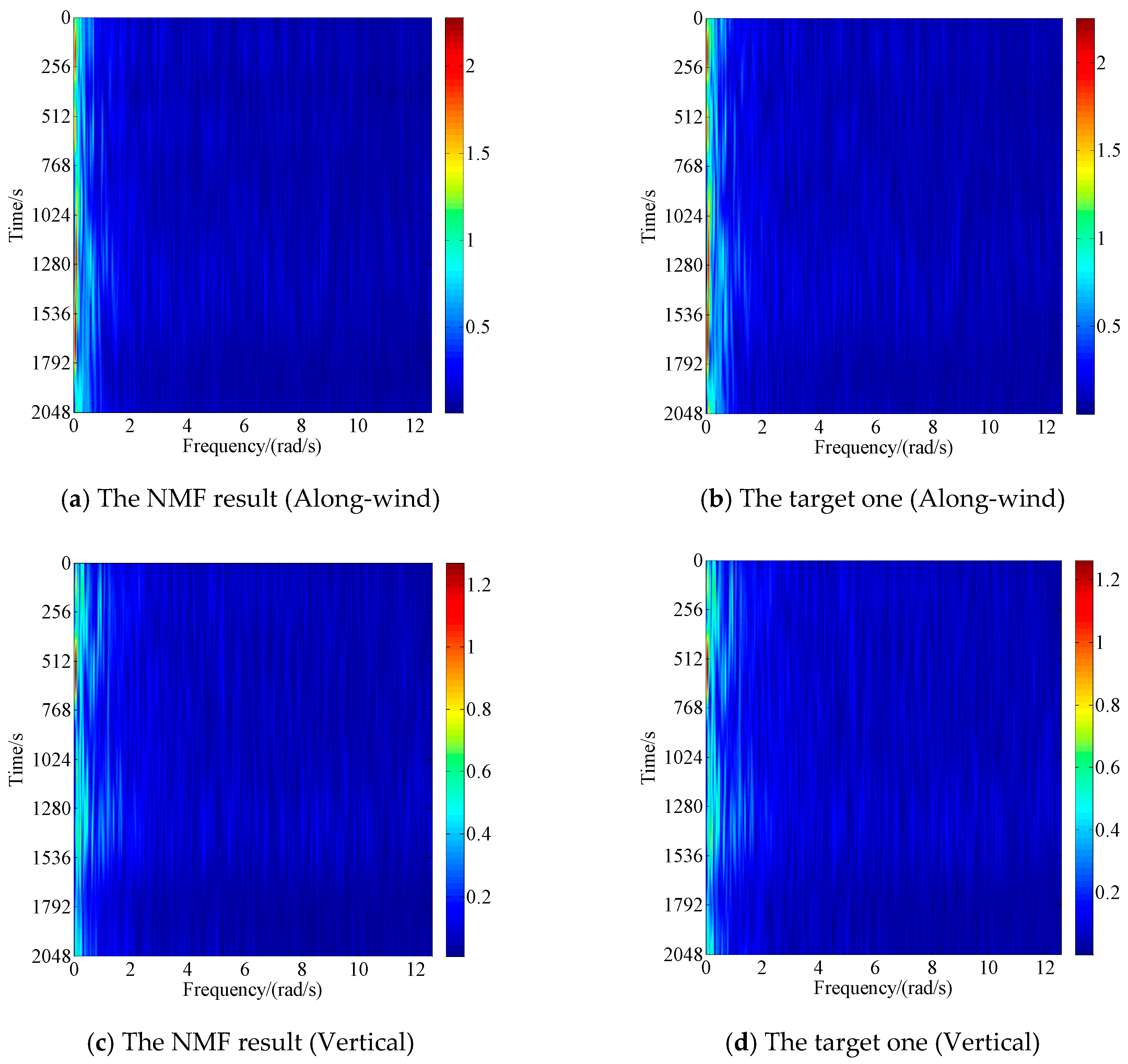
4.2. NMF of the Measured Decomposed EPSDs

The square root of the measured EPSDs in Figure 3a,c, can be factorized into the latent matrices $W$ and $V$ with the NMF. The integer $P$ in Equation (38) is taken as 8, while the iteration tolerance is taken as 10⁻⁸ in this factorization. The NMF results of the measured EPSDs are shown in Figure 5 with the target ones.

As shown in Figure 5, the NMF of the decomposed EPSD generally fit well with the targets in along-wind and vertical directions. Furthermore, the spectra snapshots of the NMF results at t = 200, 500, 1200 and 1500 s are compared with the targets. As shown in Figure 6 and Figure 7, the spectrum snapshots agree well with the targets at the specific time instants, indicating that the NMF is an effective method to factorize the measured decomposed EPSDs.

4.3. Turbulent Wind Field Simulation for the Main Girder

The Davenport exponential function model is adopted to be the coherence function for the turbulence simulation of main girder [3]:

$${\gamma }_{ij}^{}\left(\omega \right)=\exp \left(-\frac{\lambda \omega \Delta \left|i-j\right|}{2\pi \overline{U}\left(Z\right)}\right)={\xi }_{}^{\left|i-j\right|}$$

(42)

where

$$\xi =\exp \left(-\frac{\lambda \omega \Delta }{2\pi \overline{U}\left(Z\right)}\right)$$

(43)

In Equations (42) and (43), $\lambda$ represent the decay factor; $\Delta$ is the distance between the successive simulated points; $\overline{U}\left(Z,t\right)$ represents the mean wind speed, which can be obtained by averaging the $\overline{U}\left(Z,t\right)$. The mean wind speed profile at the RSB site is consistent with the power law:

$$\frac{U_2^{}}{U_1^{}}={\left(\frac{Z_2^{}}{Z_1^{}}\right)}_{}^{\alpha }$$

(44)

where $U_1^{}$ and $U_2^{}$ denote wind speeds at altitude $Z_1^{}$ and $Z_2^{}$, respectively, and $\alpha$ is a dimensionless exponent which depends on roughness of terrain, taken as measured value 0.12 herein [35]. Based on Equation (36), the explicit form of the lagged decomposed EPSD matrix $\Lambda$ can be expressed as [36]:

$$\Lambda \left(\omega ,t\right)=\sqrt{S\left(\omega ,t\right)}\left[\begin{array}{cccc}1& 0& 0& 0\\ \xi & \sqrt{1-{\xi }_{}^2}& \cdots & 0\\ ⋮& ⋮& \ddots & ⋮\\ {\xi }_{}^{n-1}& {\xi }_{}^{n-2}\sqrt{1-{\xi }_{}^2}& \cdots & \sqrt{1-{\xi }_{}^2}\end{array}\right]$$

(45)

Here, the Davenport coherence function is adopted and the decay factor is taken as seven.

Table 2. Details for non-stationary turbulent wind field simulations of main girder.

Parameter	Value	Parameter	Value
Overall length, L (m)	1490	Height of simulated points, Z (m)	69.3
Number of simulated points, n	19	Cutoff frequency, ωu (rad/s)	4π
Frequency segmentations, N	4096	Sample time interval, Δt (s)	0.25
Number of generated samples	5000	Time duration, Tu (s)	2048

lists the detailed information in the simulation.

As shown in Figure 8, 5000 samples (both in Along-wind and Vertical direction) are simulated using the measured EPSDs. Then, the auto-/cross-correlation functions are estimated using the generated samples. The generated wind fields are validated by comparing the estimated correlation functions and the target ones at various time differences $\tau$, as shown in Figure 9.

Figure 8 shows that the generated wind samples in along-wind and vertical directions exhibit prescribed non-stationary features. In Figure 9, the estimated auto-correlation functions fit well with the target one, while the discrepancy between the cross-correlation function and the target one is relatively wide. This phenomenon will be improved if many more samples are considered.

4.4. Turbulent Wind Field Simulation for Towers

As for towers, the mean wind speed approximately obeys the distribution of the exponential relationship in Equation (44). The following empirical coherence function is selected to generate the non-stationary turbulence for towers in the along-wind direction [32].

$${\gamma }_{ij}^{}\left(\omega \right)=\exp \left(-\frac{1}{2\pi }\frac{\lambda \omega \left|z_i^{}-z_j^{}\right|}{\frac{1}{2}\left[\overline{U}\left(z_i^{}\right)+\overline{U}\left(z_j^{}\right)\right]}\right)\exp \left(-i\frac{z_i^{}-z_j^{}}{v_{app}^{}}\omega \right),\left(j>k\right)$$

(46)

According to Equation (46), phase angles ${\theta }_{jm}^{}\left(\omega \right)$ in Equation (32) can be determined by:

$${\theta }_{jm}^{}\left(\omega \right)=-\frac{z_j^{}-z_m^{}}{v_{app}^{}}\omega$$

(47)

In the wind field, the apparent wave velocity $v_{app}^{}$ can be modified as [37]:

$$v_{app}^{}=\frac{\pi \left(U_j^{}+U_m^{}\right)}{C_{\theta }^{}}$$

(48)

where $U_j^{}$ and $U_m^{}$ denote the mean wind speed at different elevation; $C_{\theta }^{}$ represents the experimental appropriate coefficient [3]. Obviously, $v_{app}^{}$ is varying for the simulation points of the towers with different mean wind speeds. However, it can be approximated to be a constant by calculating the mean wind speeds on two end points, and for that the variation is usually acceptable [32].

Table 3. Details for non-stationary turbulent wind field simulations of each tower.

Parameter	Value	Parameter	Value
Overall length, L (m)	218.9	Simulation range, Z (m)	30–210
Number of simulated points, n	7	Cutoff frequency, ωu (rad/s)	4π
Frequency segmentations, N	4096	Sample time interval, Δt (s)	0.25
Number of generated samples	5000	Time duration, Tu (s)	2048

lists the detailed information in the simulation.

As shown in Figure 10, the non-stationary turbulent wind fields of towers in the along-wind direction are shown. For comparison, 5000 samples are utilized to estimate the ensemble auto-/cross-correlation functions at various time differences τ. The estimated auto-/cross-correlation functions and corresponding target ones are shown in Figure 11.

As shown in Figure 10, the non-stationary turbulent wind fields of towers are constructed from the measured EPSD in along-wind direction with the coherence function in Equation (46). It is seen that the estimated correlation functions generally fit well with the target ones in Figure 11, indicating the reliability of the generated non-stationary turbulent wind fields of the towers.

5. Conclusions

The existing FFT-aided NMF-based SRM, which cannot simulate the vertical turbulent wind field, has been updated to simulate a non-stationary turbulent wind field in both horizontal and vertical directions. NMF can be utilized to decouple the EPSD matrix, the FFT technique can be then utilized to improve the simulation efficiency of the non-stationary SRM. The turbulent wind fields of the RSB are generated based on the field-measured EPSDs during typhoon Wipha. The non-stationary turbulent wind fields for towers are generated considering the coherence function with the phase angles. Relative comparisons are conducted to validate the reliability and accuracy of the generated wind fields. The following conclusions can be drawn accordingly:

• The existed NMF-based SRM for horizontal non-stationary turbulent wind field simulation is updated to also generate the vertical non-stationary turbulent wind field. With the aid of the FFT, the simulation efficiency is enhanced.
• In the NMF-based SRM, the phase angles can be considered in the coherence functions. The complex EPSD matrix can be transformed into the real modulus matrix after the phase was separated. With this treatment, the efficiency of decomposition can be improved.
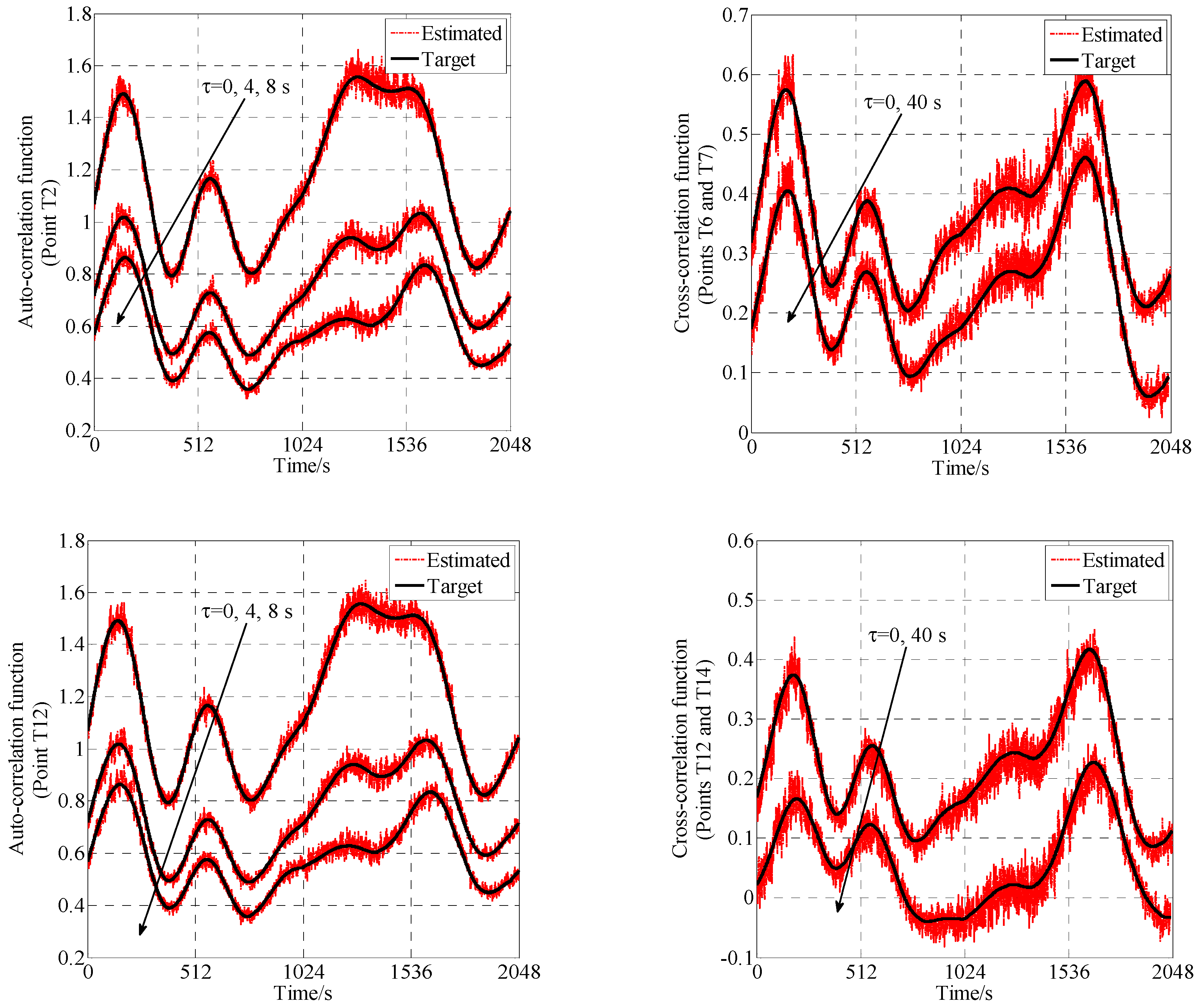
• The estimated auto-/cross-correlation functions generally fit well with the target ones, validating the effectiveness and reliability of the non-stationary turbulent wind fields generated. The presented wind field simulation method can provide research basis for non-stationary buffeting analysis of the RSB.

References

1. Bocciolone, M.; Cheli, F.; Curami, A.; Zasso, A. Wind measurements on the Humber Bridge and numerical simulations. J. Wind Eng. Ind. Aerodyn. 1992, 42, 1393–1404. [Google Scholar] [CrossRef]
2. Kovacs, I.; Svensson, H.S.; Jordet, E. Analytical aerodynamic investigation of cable-stayed Helgeland bridge. J. Struct. Eng. 1992, 118, 147–168. [Google Scholar] [CrossRef]
3. Simiu, E.; Scanlan, R.H. Wind Effects on Structures; Wiley: New York, NY, USA, 1978. [Google Scholar]
4. Niemann, H.J.; Hoffer, R. Nonlinear Effects in the Buffeting Program: A State of the Art in Wind Engineering. In Proceedings of the Ninth International Conference on Wind Engineering, New Delhi, India, 9–13 January 1995. [Google Scholar]
5. Yang, W.W.; Chang, T.Y.P.; Chang, C.C. An efficient wind field simulation technique for bridges. J. Wind Eng. Ind. Aerodyn. 1997, 67, 697–708. [Google Scholar] [CrossRef]
6. Su, C.; Fan, X.; He, T. Wind-induced vibration analysis of a cable-stayed bridge during erection by a modified time-domain method. J. Sound Vib. 2007, 303, 330–342. [Google Scholar] [CrossRef]
7. Mao, J.X.; Wang, H.; Feng, D.M.; Tao, T.Y.; Zheng, W.Z. Investigation of dynamic properties of long-span cable-stayed bridges based on one-year monitoring data under normal operating condition. Struct. Control Health Monit. 2018, 25, e2146. [Google Scholar] [CrossRef]
8. Mao, J.X.; Wang, H.; Fu, Y.G.; Spencer, B.F., Jr. Automated modal identification using principal component and cluster analysis: Application to a long-span cable-stayed bridge. Struct. Control Health Monit. 2019, 26, e2430. [Google Scholar] [CrossRef]
9. Chen, X.; Matsumoto, M.; Kareem, A. Time domain flutter and buffeting response analysis of bridges. J. Eng. Mech. 2000, 126, 7–16. [Google Scholar] [CrossRef] [Green Version]
10. Deodatis, G. Simulation of ergodic multivariate stochastic processes. J. Eng. Mech. 1996, 122, 778–787. [Google Scholar] [CrossRef]
11. Li, Y.; Kareem, A. Simulation of multivariate random processes: Hybrid DFT and digital filtering approach. J. Eng. Mech. 1993, 119, 1078–1098. [Google Scholar] [CrossRef]
12. Chen, J.; Hui, M.C.H.; Xu, Y.L. A comparative study of stationary and non-stationary wind models using field measurements. Bound. Layer Meteorol. 2007, 122, 105–121. [Google Scholar] [CrossRef]
13. Kareem, A. The changing dynamics of aerodynamics: New frontiers. In Proceedings of the 7th Asia-Pacific Conference on Wind Engineering (APCWQ-VII), Taiwan, China, 8–12 November 2009. [Google Scholar]
14. Wang, H.; Wu, T.; Tao, T.Y.; Li, A.Q.; Kareem, A. Measurements and analysis of non-stationary wind characteristics at Sutong Bridge in Typhoon Damrey. J. Wind Eng. Ind. Aerodyn. 2016, 151, 100–106. [Google Scholar] [CrossRef] [Green Version]
15. Deodatis, G. Non-stationary stochastic vector processes: Seismic ground motion applications. Probab. Eng. Mech. 1996, 11, 149–167. [Google Scholar] [CrossRef]
16. Li, Y.; Kareem, A. Simulation of multivariate nonstationary random processes by FFT. J. Eng. Mech. 1991, 117, 1037–1058. [Google Scholar] [CrossRef]
17. Huang, G. Application of proper orthogonal decomposition in fast Fourier transform-assisted multivariate nonstationary process simulation. J. Eng. Mech. 2015, 141, 04015015. [Google Scholar] [CrossRef]
18. Li, Y.; Togbenou, K.; Xiang, H.; Chen, N. Simulation of non-stationary wind velocity field on bridges based on Taylor series. J. Wind Eng. Ind. Aerodyn. 2017, 169, 117–127. [Google Scholar] [CrossRef]
19. Wang, H.; Xu, Z.D.; Feng, D.M.; Tao, T.Y. Non-stationary turbulent wind field simulation of bridge deck using non-negative matrix factorization. J. Wind Eng. Ind. Aerodyn. 2019, 188, 235–246. [Google Scholar] [CrossRef]
20. Wang, H.; Li, A.Q.; Huang, R.X.; Xie, J.; Xie, Y.S. Field measurements on wind characteristics of typhoon wipha at the runyang suspension bridge. Eng. Mech. 2009, 26, 128–133. (In Chinese) [Google Scholar]
21. Xu, Z.D.; Wang, H.; Wu, T.; Tao, T.Y.; Mao, J.X. Wind characteristics at Sutong Bridge site using 8-year field measurement data. Wind Struct. 2017, 25, 195–214. [Google Scholar]
22. Bendat, J.S.; Piersol, A.G. Random Data: Analysis and Measurement Procedures, 4th ed.; Wiley: New York, NY, USA, 2011. [Google Scholar]
23. Spanos, P.D.; Failla, G. Evolutionary spectra estimation using wavelets. J. Eng. Mech. 2004, 130, 952–960. [Google Scholar] [CrossRef]
24. Spanos, P.D.; Tezcan, J.; Tratskas, P. Stochastic processes evolutionary spectrum estimation via harmonic wavelets. Comput. Methods Appl. Mech. Eng. 2005, 194, 1367–1383. [Google Scholar] [CrossRef]
25. Wang, H.; Xu, Z.D.; Wu, T.; Mao, J.X. Evolutionary power spectral density of recorded typhoons at Sutong Bridge using harmonic wavelets. J. Wind Eng. Ind. Aerodyn. 2018, 177, 197–212. [Google Scholar] [CrossRef] [Green Version]
26. Welch, P. The use of fast Fourier transform for the estimation of power spectra: A method based on time averaging over short, modified periodograms. IEEE Trans. Audio Electroacoust. 1967, 15, 70–73. [Google Scholar] [CrossRef] [Green Version]
27. Priestley, M.B. Evolutionary spectra and non-stationary processes. J. R. Stat. Soc. 1965, 27, 204–237. [Google Scholar] [CrossRef]
28. Lee, D.D.; Seung, H.S. Learning the parts of objects by non-negative matrix factorization. Nature 1999, 401, 788–791. [Google Scholar] [CrossRef]
29. Berry, M.W.; Browne, M.; Langville, A.N.; Pauca, V.P.; Plemmons, R.J. Algorithms and applications for approximate nonnegative matrix factorization. Comput. Stat. Data Anal. 2007, 52, 155–173. [Google Scholar] [CrossRef] [Green Version]
30. Lee, D.D.; Seung, H.S. Algorithms for non-negative matrix factorization. Adv. Neural Inf. Process. Syst. 2001, 13, 556–562. [Google Scholar]
31. Gao, Y.; Wu, Y.; Li, D.; Liu, H.; Zhang, N. An improved approximation for the spectral representation method in the simulation of spatially varying ground motions. Probab. Eng. Mech. 2012, 29, 7–15. [Google Scholar] [CrossRef]
32. Huang, G.; Liao, H.; Li, M. New formulation of Cholesky decomposition and applications in stochastic simulation. Probab. Eng. Mech. 2013, 34, 40–47. [Google Scholar] [CrossRef]
33. Kiureghian, A. A coherency model for spatially varying ground motions. Earthq. Eng. Struct. Dyn. 1996, 25, 99–111. [Google Scholar] [CrossRef]
34. Xu, Y.L.; Hu, L.; Kareem, A. Conditional simulation of nonstationary fluctuating wind speeds for long-span bridges. J. Eng. Mech. 2012, 140, 61–73. [Google Scholar] [CrossRef]
35. Wang, H.; Zong, Z.H.; Li, A.Q.; Tong, T.; Niu, J.; Deng, W.P. Digital simulation of 3D turbulence wind field of Sutong Bridge based on measured wind spectra. J. Zhejiang Univ. Sci. A 2012, 13, 91–104. [Google Scholar] [CrossRef]
36. Cao, Y.; Xiang, H.; Zhou, Y. Simulation of stochastic wind velocity field on long-span bridges. J. Eng. Mech. 2000, 126, 1–6. [Google Scholar] [CrossRef]
37. Di Paola, M. Digital simulation of wind field velocity. J. Wind Eng. Ind. Aerodyn. 1998, 74–76, 91–109. [Google Scholar] [CrossRef]
Figure 1. Location of the Runyang Suspension Bridge (RSB).
Applsci 09 05506 g001
Figure 2. Field measured wind data during Typhoon Wipha.
Applsci 09 05506 g002
Figure 3. Estimating and validating the evolutionary power spectral density (EPSD) of the measured turbulence.
Applsci 09 05506 g003
Figure 4. Simulated points in the RSB (Unit: m).
Applsci 09 05506 g004
Figure 5. The non-negative matrix factorization (NMF) of the decomposed EPSDs and the targets.
Applsci 09 05506 g005
Figure 6. Spectrum snapshots of the decomposed EPSD (along-wind).
Applsci 09 05506 g006
Figure 7. Spectrum snapshots of the decomposed EPSD (vertical).
Applsci 09 05506 g007
Figure 8. The generated samples for the main girder.
Applsci 09 05506 g008aApplsci 09 05506 g008b
Figure 9. Comparison of estimated correlation functions and target ones (5000 samples).
Applsci 09 05506 g009
Figure 10. Simulation of non-stationary turbulence for towers.
Applsci 09 05506 g010aApplsci 09 05506 g010b
Figure 11. Comparison of estimated correlation functions and target ones (5000 samples).
Applsci 09 05506 g011