Article

Development of Hybrid Machine Learning Models for Predicting the Critical Buckling Load of I-Shaped Cellular Beams

1
University of Transport Technology, Hanoi 100000, Vietnam
2
Institute of Research and Development, Duy Tan University, Da Nang 550000, Vietnam
3
Faculty of Engineering, Vietnam National University of Agriculture, Gia Lam, Hanoi 100000, Vietnam
4
Thuyloi University, Hanoi 100000, Vietnam
*
Authors to whom correspondence should be addressed.
Appl. Sci. 2019, 9(24), 5458; https://doi.org/10.3390/app9245458
Submission received: 22 October 2019 / Revised: 4 December 2019 / Accepted: 11 December 2019 / Published: 12 December 2019
(This article belongs to the Special Issue Meta-heuristic Algorithms in Engineering)

Abstract

:
The principal purpose of this work is to develop three hybrid machine learning (ML) algorithms, namely ANFIS-RCSA, ANFIS-CA, and ANFIS-SFLA which are a combination of adaptive neuro-fuzzy inference system (ANFIS) with metaheuristic optimization techniques such as real-coded simulated annealing (RCSA), cultural algorithm (CA) and shuffled frog leaping algorithm (SFLA), respectively, to predict the critical buckling load of I-shaped cellular steel beams with circular openings. For this purpose, the existing database of buckling tests on I-shaped steel beams were extracted from the available literature and used to generate the datasets for modeling. Eight inputs, considered as independent variables, including the beam length, beam end-opening distance, opening diameter, inter-opening distance, section height, web thickness, flange width, and flange thickness, as well as one output of the critical buckling load of cellular steel beams considered as a dependent variable, were used in the datasets. Three quality assessment criteria, namely correlation coefficient (R), root mean squared error (RMSE) and mean absolute error (MAE) were employed for assessment of three developed hybrid ML models. The obtained results indicate that all three hybrid ML models have a strong ability to predict the buckling load of steel beams with circular openings, but ANFIS-SFLA (R = 0.960, RMSE = 0.040 and MAE = 0.017) exhibits the best effectiveness as compared with other hybrid models. In addition, sensitivity analysis was investigated and compared with linear statistical correlation between inputs and output to validate the importance of input variables in the models. The sensitivity results show that the most influenced variable affecting beam buckling capacity is the beam length, following by the flange width, the flange thickness, and the web thickness, respectively. This study shows that the hybrid ML techniques could help in establishing a robust numerical tool for beam buckling analysis. The proposed methodology is also promising to predict other types of failure, as well as other types of perforated beams.

1. Introduction

In the field of structural engineering, the use of steel cellular beams has gained widespread attention thanks to their economic and aesthetic advantages [1,2]. Currently, as a result of their particular design, they are widely used in structural systems subject to bending or funicular structures [3,4,5]. The I-shaped cellular steel beams are formed from standard I-section beams by cutting regularly circular openings, a specific geometrical feature that results in numerous advantages, for example, the optimum self-weight-depth ratio, improvement of flexural stiffness, or larger section modulus [3]. Furthermore, in combination with the significant compressive strength of concrete slab, the flexural resistance of composite cellular beam is significantly improved [2,6].
Safety at construction projects is an important matter, which is strongly related to the stability of the constituent structural elements, in other words, the bucking behavior of cellular beams. In the literature, various experimental, analytical, and numerical studies have been performed to investigate the buckling behavior of beams [7,8,9]. As regards to I-shaped beams [5], a numerical investigation was carried out on the buckling modes of cellular beams using ABAQUS software. An important change in the failure loads was observed when subjected to a combination of web distortional and web-post buckling failing modes. In addition, the lateral-torsional buckling behavior of cellular beams was investigated by Sonck and Belis [10] who took into account the effect of the residual stress. In another attempt, the bucking behavior of steel I-shaped cellular beams was discussed and numerous parametric studies were used to assess the variation of the moment-gradient coefficient [4]. This study also provided a modification to evaluate the critical lateral buckling moment of the analyzed beams under different loading conditions. Last but not least, an experimental and analytical study on the behavior and strength of steel beams was performed by Tsavdaridis and D’Mello [11]. An empirical formula with the ability to predict ultimate vertical shear load strength was proposed using a finite element approach in a parametric analysis. In general, the mechanical simulation approach or laboratory experiments can only be applied to a limited case [12]. Moreover, they are costly and require significant amounts of time [13]. Therefore, the development of a straightforward and rapid numerical tool to solve the bucking behavior problem of steel I-shaped cellular beams is imperative [1,12,14].
In the past few decades, machine learning (ML) approaches have been the subject of extensive interest and expanding research in the field of materials science [15], especially in structural engineering [8,9,16,17,18,19]. Currently, the rapid and constant development of computational software and hardware has facilitated the development of numerous alternative computer-aided data mining approaches. For example, Reddy [20] developed an artificial neural networks (ANN) algorithm for predicting the hardness of concrete reinforced with randomly oriented steel fibers. The proposed ANN model has been compared with selected experiments and has shown an extremely high utilization rate. In addition, other studies [21,22,23,24,25,26] have also confirmed the strong predictability of different ML models for the behavior of structural elements and different materials in the field of mechanics under different solicitations [8,9,27,28,29,30].
Consequently, the main objective of this paper is the development and comparison of different hybrid ML models to predict the critical buckling load of I-shaped steel cellular beams. In this regard, three hybrid ML models, namely ANFIS-RCSA, ANFIS-CA, and ANFIS-SFLA, which are a combination of adaptive neuro-fuzzy inference system (ANFIS) with metaheuristic optimization techniques such as real-coded simulated Annealing (RCSA), cultural algorithm (CA) and shuffled frog leaping algorithm (SFLA), were developed and applied. Performance of these models was validated and compared using well-known statistical measures such as correlation coefficient (R), root mean squared error (RMSE), and mean absolute error (MAE). Then, the best prediction model was used to perform sensitivity analysis to deduce the factors that greatly affect the predicted critical buckling load.

2. Materials and Methods

2.1. Description of Cellular Beams and Selection of Variables for Training ML Models

The data used in this work was extracted from a validated finite element (FE) model, previously introduced in the literature by Abambres et al. [31]. The goodness of using data from a validated FE solver instead of experiments for training ML models has been proved in various investigations such as Mallela and Upadhyay [32] and Sadovský and Soares [33]. In this study, a total number of 3645 FE configurations on buckling behavior of I-section beams with circular openings were extracted to form the dataset for training the ML models, involving eight inputs and one output, detailed as follows:
The cross section of the beams is I-shaped under the four controlled parameters, section height, flange width, thickness, and web thickness (Figure 1). As indicated in Table 1, the section height varies from 420 mm to 700 mm (560 mm of mean value and 114.33 mm of standard deviation). The web thickness ranges from 9 mm to 15 mm (mean value of 12 mm and standard deviation of 2.45 mm). The flange width varies from 162 mm to 270 mm (216 mm of mean value and 44.10 mm of standard deviation). The flange thickness ranges from 15 mm to 25 mm (mean value of 20 mm and standard deviation of 4.08 mm).
For a beam with given length, various circular openings had been cut regularly along the beam axis, under three controlled parameters such as beam end-opening distance, opening diameter, and inter-opening distance (Figure 1). The beam end-opening distance ranges from 12 mm to 718 mm (mean value of 265.36 mm and standard deviation of 157.46 mm). The opening diameter varies from 247 mm to 560 mm (383.56 mm of mean value and 92.98 mm of standard deviation). The inter-opening distance ranges from 24.70 mm to 274.40 mm (mean value of 112.51 mm and standard deviation of 68.51 mm). Finally, the beam length varies from 4000 mm to 8000 mm (6000 mm of mean value and 1410 mm of standard deviation).
The cellular beams were subjected to a uniformly distributed load, as schematized in Figure 1. The pinned-pinned boundary condition was applied for the beams. It should be noticed that twisting rotation at both ends of the beams was not allowed to expose the in-plane’s rotation and translation influence. The constituent material of the beams is steel under two controlled elastic constants such as the Young’s modulus of 210 GPa and the Poisson’s coefficient of 0.30. Quad shell elements containing 4 nodes and 6 degrees of freedom at each node (3 for translations and 3 for rotations) were employed to discretize the beams in the FE scheme. The FE simulations and numerical results are obtained using ABAQUS [34]. It has been proved that such element can correctly model thin and moderate thickness shell structures with elastic and elasto-plastic behaviors of materials [35]. The flanges were discretized by 12 elements, whereas the discretization of the web along the span were performed with element size of about H/20 (Figure 2). In addition, a pinned condition was adopted for discretization of the web-flange connection to form a safe lower bound which was independent of the flange size and type of weld, as recommended by Tsavdaridis and D’Mello [11]. The critical buckling load, or the output of the ML models, varied from 26.40 N/m to 1361.70 N/m (mean value of 225.68 N/m and standard deviation of 80.87 N/m). It should be pointed out that initial imperfections corresponding to geometry or fluctuations of material and residual stresses were not studied [36].
The data used in this work were scaled into the range [0, 1] in order to minimize bias within the dataset between variables. For the jth variable, the expression for scaling is defined as follow:
V j s c a l e d = V j r a w n j m j n j ,
where scaling parameters m and n are also indicated in Table 1. In general, ML related problems often use this technique to transform the dataset into a uniform range to reduce numerical bias [9,37]. It should be noted that a reserve transformation could be deduced for converting data from the scaling space to the raw one.
The relationship between input and output variables is plotted in Figure 3. It is observed that no particular correlations are found between two inputs or between inputs and the output.

2.2. Adaptive Neuro-Fuzzy Inference System (ANFIS)

AFNIS is a multilayered network based on neural network learning algorithms and fuzzy reasoning [38,39,40,41]. Thanks to its ability to combine the a fuzzy system with numerical power of adaptive neural networks, ANFIS has demonstrated its ability to model many problems in the field of science such as prediction of the geopolymer concrete compressive strength [42], the Marshal parameters of stone matrix asphalt mixtures [43], the buckling damage of structural members [9], the dynamic loadings of power systems [44,45], the buckling damage of steel columns under axial compression [8], the International Roughness Index of pavements [46], the blast-induced air-overpressure in quarry blasting sites [47], the traffic air pollution [48], and the flocculation-dewatering performance of fine mineral tailings [49]. ANFIS has a good ability to learn, build, expand and classify as the advantage of ANFIS is that it allows the fuzzy rules to be extracted from numerical data and is appropriate for formulating a rule base. Moreover, ANFIS can adjust the complex movement of human intelligence into fuzzy systems. However, computation time is one disadvantage of ANFIS, especially in the training process and identification of parameters.

2.3. Real-Coded Simulated Annealing (RCSA)

RCSA is a powerful tool for global optimization. On the basis of the similarity between a search algorithm and the process of annealing in metallurgy, the first idea of simulated annealing (SA) appeared in the work of Metropolis et al. [50] as a simulation algorithm. The search algorithm of SA focuses on identifying the solutions without ignoring better solutions that can be found later. Kirkpatrick et al. [51] and Cerny et al. [52] used Metropolis’ idea to search for feasible solutions and converge to an optimal solution called “simulated annealing”.
Similar to a cooling process, the algorithm simulates a steady temperature decrease until the system converges to a stable state, avoiding the inclusion of defects when cooling too quickly or too slowly [53]. While annealing is the process of first heating of a solid and then cooling it down slowly, in SA, the temperature is kept variable to simulate the heating mechanism. Specifically, the temperature is set high at the initial step and then “cool down” occurs slowly. The initial heating essentially helps to avoid a trap in a local minimum [54]. As the temperature decreases, its new structure becomes increasingly fixed, thus, firmly setting the final properties. In the end, the free energy of the system is minimized, imitating how a minimum is reached during the annealing process, eventually resulting in an optimized solution [55,56]. For more information on SA, the reader is referred to the published studies [57,58]. In this study, RCSA was used to optimize the parameters of the ANFIS to develop a hybrid model, namely ANFIS-RCSA.

2.4. Cultural Algorithm (CA)

Derived from observations of cultural evolution in real life, CA is a computational and optimization algorithm [59,60]. It is helpful to deal with complex calculations or optimization of the searching process. CA is inspired from the human culture development at two levels of evolutionary. The first one, the macro level, takes place in the beliefs space and the second one, the micro level, occurs in the space of people [61].
In brief, CA consists of three components. First, it is the evolved social population and the evaluation, reproduction, and modification mechanisms. Secondly, the belief space represented for the bias was acquired by the population during the problem-solving process. The communication protocol, the third component, is where the interaction of the population and their beliefs is identified [62].
Precisely, the process starts by initializing, firstly, the belief, as well as the population spaces. In the next step, the algorithm is repeated for each generation before achieving the termination condition. The performance function is used to evaluate the individuals. The influence function and the acceptance function are mediums to communicate between two levels of CA. The two functions identify and select the individuals from the current population to influence the belief space. The experiences of selected ones are generalized and applied to adjust the current beliefs via the updated function. The generated beliefs are further used to guide and influence the next generation through the evolutionary process [60].
CA is popularly used to perform complex calculations of the optimization search algorithm [63] and in many other applications [62,64]. In this study, CA was used to optimize the parameters of the ANFIS to develop a hybrid model, namely ANFIS-CA.

2.5. Shuffled Frog Leaping Algorithm (SFLA)

SFLA belongs to the metaheuristic algorithms based on frog’s behavior. It was first introduced in the work of Eusuff and Lansey [65] to optimize the water distribution network. The frog’s behavior in seeking food is the main concept of SFLA. Moreover, the advantages of other optimization methods, such as particle swarm optimization (PSO) or genetic algorithm (GA), could also be found in SFLA algorithm [66,67]. In the SFLA optimization process, the global and local search mechanisms are properly compromised. Several subsets (memeplex) divide the frog population and perform in the local search. In each memeplex, the worst frog is replaced by the best one [68,69].
Numerous complex optimization problems can be solved by SFLA, such as multimodal problems, nonlinear and non-differential [67,70,71,72]. This method can achieve better results through the distribution of water resources, the fuzzy or multivariable PID controller, and the repair of bridge-deck [73,74]. In this study, SFLA was used to optimize the parameters of the ANFIS to develop a hybrid model, namely ANFIS-SFLA.

2.6. Performance Indicators

The performance of three hybrid ML models was evaluated by three statistical criteria, namely RMSE, R, and MAE [7,75,76,77]. The R-value indicates the correlation between the predicted values, given by the ML models, and the actual values [78]. RMSE is the average squared difference between the predicted and actual values [19,79,80]. MAE measures the average of absolute difference between outputs (predicted values) and targets (actual values) [81,82,83]. On the one hand, higher R indicates a better model [84]. On the other hand, lower RMSE and MAE indicate a better model [85,86]. The formulas are defined as follow [87,88,89,90]:
MAE = i = 1 n | p i v i | n
RMSE = i = 1 n ( p i v i ) 2 n
R = i = 1 n ( p i q ) ( v i v _ ) i = 1 n ( p i q ) 2 i = 1 n ( v i v _ ) 2
where n refers to the number of samples in the dataset; pi and q are the values and means of the predicted critical buckling load, respectively; and vi and v are the individual and mean values of the actual critical buckling load, respectively.

2.7. Methodology Flow Chart

The work’s methodology (Figure 4) is described below, containing five main steps:
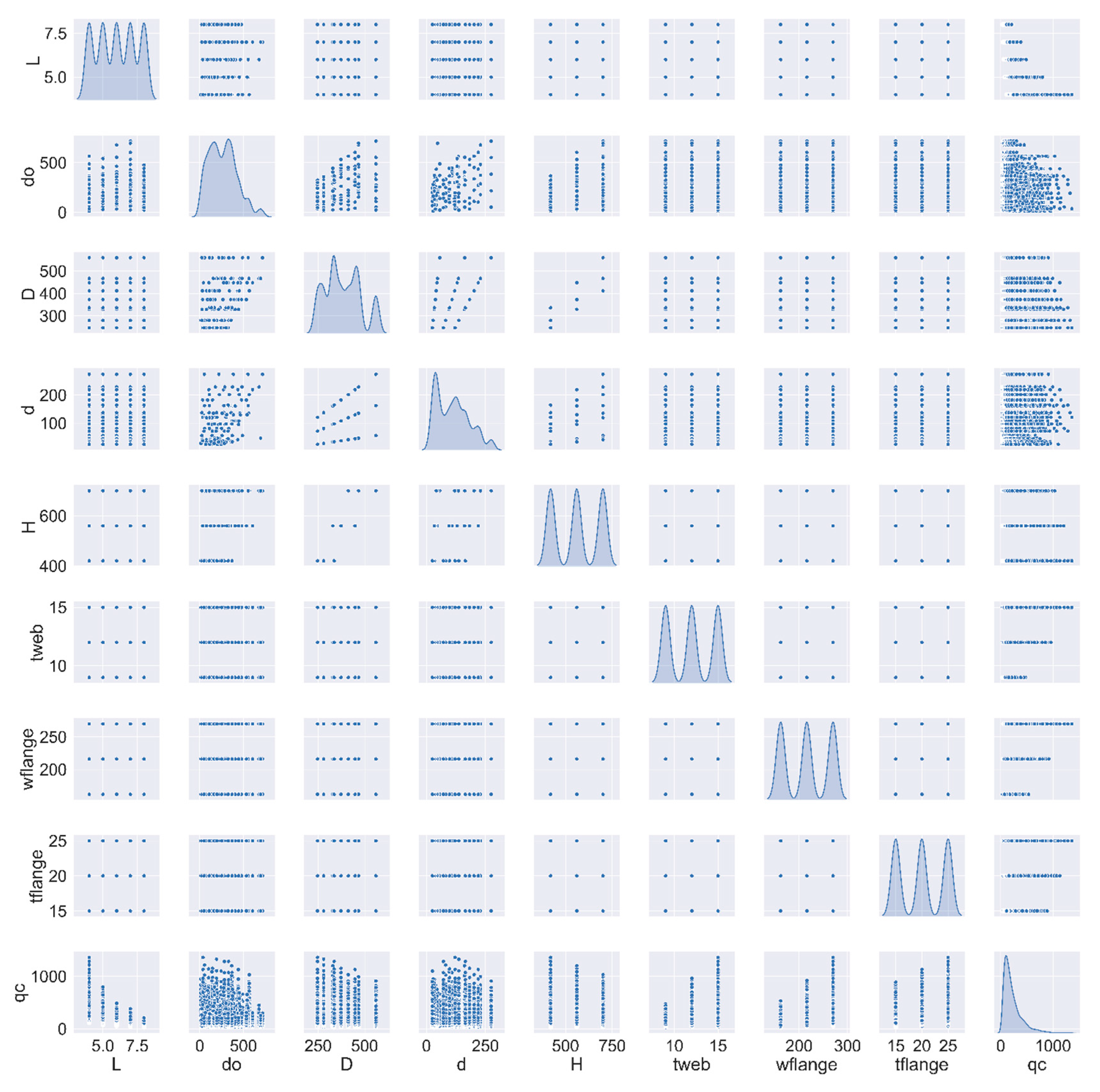
  • Collecting data: Input parameters including beam length (L), beam end opening distance (d0), opening diameter (D), inter-opening distance (d), section height (H), web thickness (tweb), flange width (wflange), flange thickness (tflange), and the output parameter of the critical buckling load (qc) were collected from the literature published in Abambres et al. [31].
  • Dataset preparation to train ML models: The input and output parameters were used to create a complete set of data. A number of 70% data (2551 training samples) were extracted from the initial dataset for training the ML models. The remaining 30% data (1094 testing samples) were used for validation the AI models.
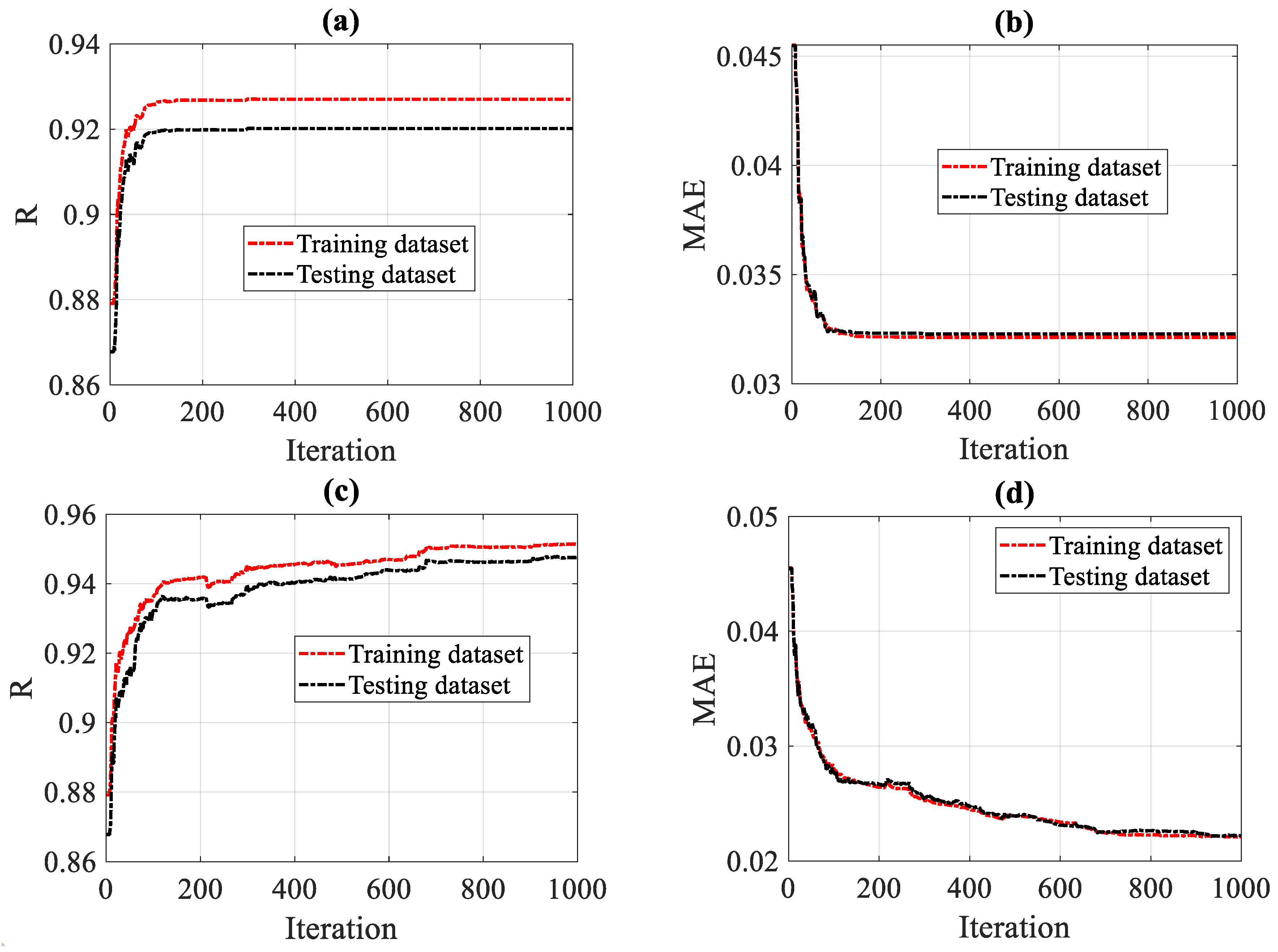
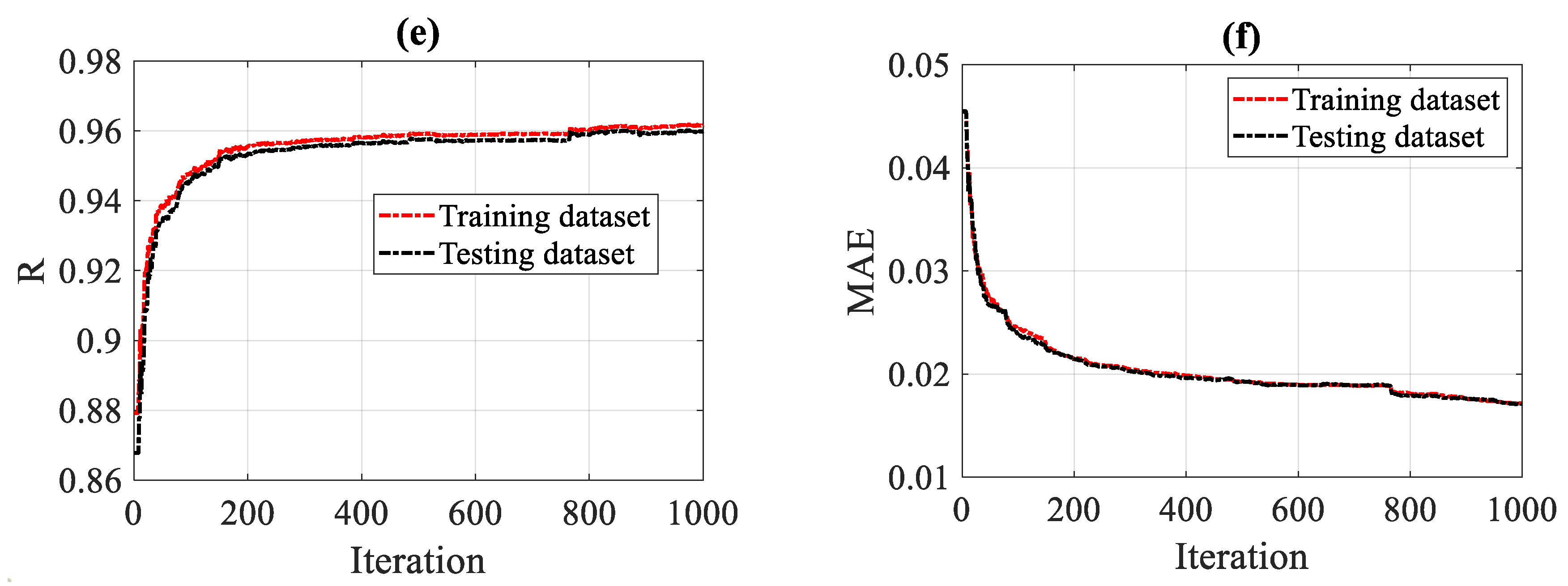
  • Training models: The ML models were trained using the training dataset. Three ML algorithms based on ANFIS with three optimization methods RCSA, CA, and SFLA. The concepts of these models were introduced in the previous sections. This step was repeated until the models successfully trained within a preselected tolerance error criterion.
  • Models validation: After successfully training three ML models, the validation process was performed using the testing dataset. The models were verified using different statistical measures such as RMSE, MAE. and R.
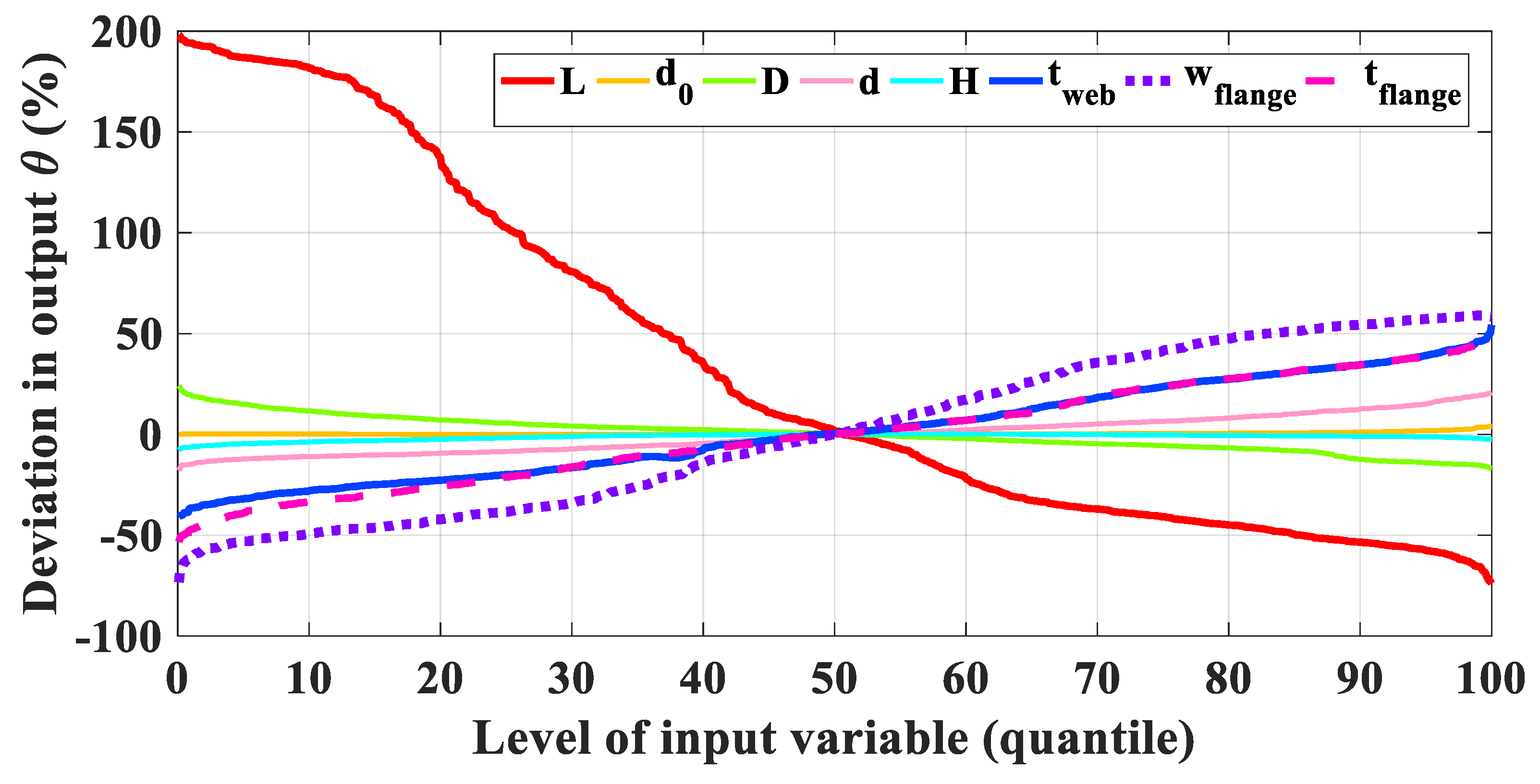
  • Sensitivity analysis: After validation of the ML models, the sensitivity of input parameters was performed using the best model to identify the influence between input parameters and the critical buckling load of I-shaped cellular beams.

3. Results and Discussions

3.1. Building the Hybrid ML Models

Performance of a ML model highly depends on the choice of its parameters. In this study, the parameters for the ANFIS model was selected and used to develop the hybrid models after trial and error test on training dataset (Table 2). In addition, the performance of the model can be affected by the sampling strategy of datasets; thus, the sampling strategy was analyzed by randomly picking data points in the whole dataset to reduce the effect of randomness on the model’s performance. Over 100 times of simulation was ran to get the best performance of the models corresponding to the highest values of R and lowest values of MAE and RMSE. Different optimization techniques such as RCSA, CA, and SFLA were applied for optimizing the parameters of ANFIS and the corresponding parameters of these techniques are summarized in Table 3, Table 4 and Table 5, respectively. Evaluation of cost functions with respect to R and MAE using ANFIS-RCSA, ANFIS-CA, and ANFIS-SFLA for predicting the critical buckling load of I-shaped beams are presented in Figure 5. For each model, the stopping condition was chosen as 1000 iterations. It is shown that ANFIS-RCSA reaches the state of convergence over 100 iterations, whereas it is about 800 iterations for ANFIS-CA and ANFIS-SFLA.
On the basis of the training phase analysis, it is observed that selection of optimal parameters for training the predictive ML models is highly important before any further investigation. The stopping iteration of a model is also an important factor as it could directly affect the computation time, as well as the efficiency of an algorithm. A more appropriate convergence criterion should be included in the ANFIS-SFLA code in order to better track the information of the cost function (i.e., R, RMSE, and MAE). By default, the 1000 iterations criterion as the stopping condition is selected because it provided a reasonable computation time. Such criterion should be modified in further studies such that the error between the cost function of iteration (i + 1) and iteration (i) exposes no more than a given threshold (i.e., 1% for example). In general, it can be concluded that ANFIS-SFLA is the best ML predictor, following by ANFIS-CA and ANFIS-RCSA in the training phase.

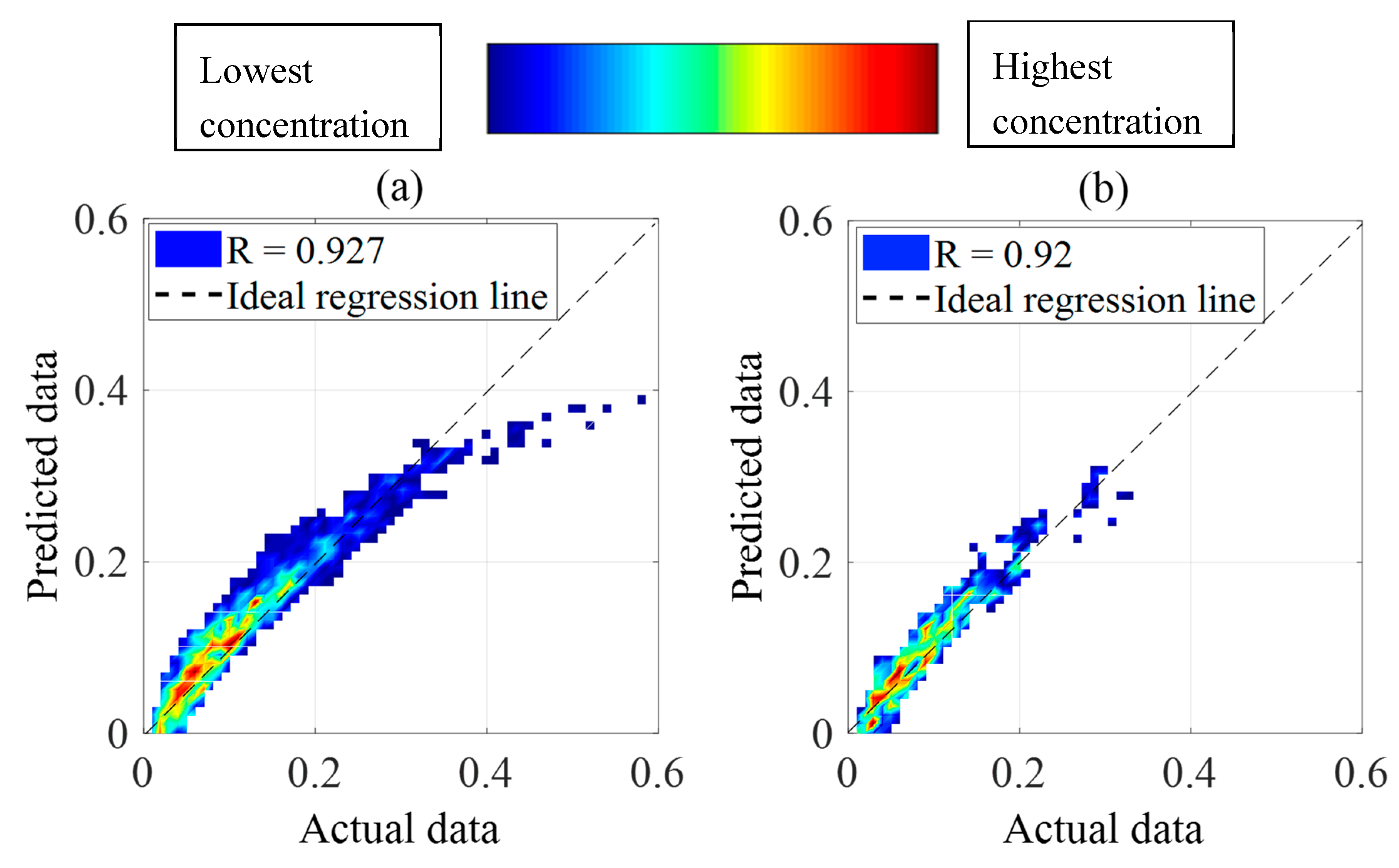
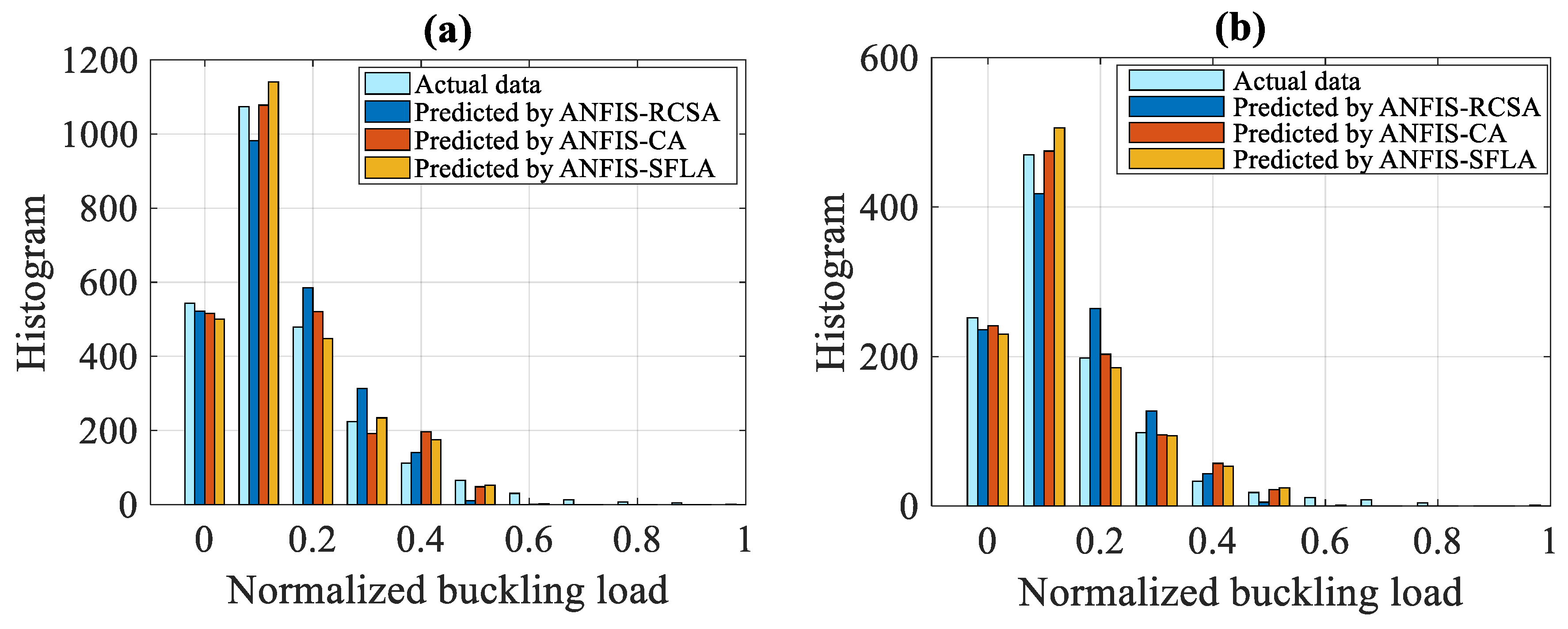
3.2. Validating the Hybrid ML Models

Validation of the hybrid models was done using both training and testing datasets, as shown in Figure 6. The ideal regression lines are in discontinuous, whereas the R-values between predicted and actual critical buckling load are given in Table 6. The results are obtained after 1000 iterations for all hybrid ML models. The clouds of data points are given in color in order to better illustrate the concentration of points. The correlation results analysis shows that the R values vary from 0.927 to 0.962 for the training dataset and from 0.920 to 0.960 for the testing dataset. These results display a very good prediction performance of all the models, but ANFIS-SFLA is found to be the best predictor compared with other models.
A detailed summary of the prediction capability of ANFIS-RCSA, ANFIS-CA, and ANFIS-SFLA is presented in Table 6, whereas “Error Mean” is the mean of all relative errors, “Error StD” is the standard deviation of relative errors and “Slope” represents the slope between the ideal regression line and the linear fit given by the models. The results also confirm that ANFIS-SFLA is superior to ANFIS-RCSA and ANFIS-CA in predicting the critical buckling load of I-shaped beams.
Histograms of the scaled critical buckling load of I-shaped beams of both actual and predicted values issued from ANFIS-RCSA, ANFIS-CA, and ANFIS-SFLA algorithms is presented in Figure 7 for both training and testing datasets The results show that a high concentration of the values is found in the [0, 0.5] interval, which emphasize the values around 0.1. This is also confirmed by the red color from Figure 6. It is worth noticed that the better correlation between actual and predicted critical buckling load is represented by the height of bars. An equally height of bars for a given value of critical buckling load means a perfect correlation (R = 1). More precisely, the error histograms between actual and predicted critical buckling load simulated by ANFIS-RCSA, ANFIS-CA, and ANFIS-SFLA are presented in Figure 8. The errors are found in the [₋0.1, 0.1] range, which speaks for about 10% of error. ANFIS-SFLA is again proved as the best predictor, following by ANFIS-CA and ANFIS-RCSA, respectively. This could be easily observed by the highest value centered on 0 (ANFIS-SFLA) and the narrow curves (ANFIS-SFLA and ANFIS-CA) of about 2% of error. In general, in terms of six error criteria, three models perform well, but ANFIS-SFLA is shown to be superior to ANFIS-RCSA and ANFIS-CA for predicting the critical buckling load of I-shaped beams. On the basis of a comparison with the previous published study by Abambres et al. [31] using the same datasets but different ML model, namely ANN, it can be observed that although the R values of ANFIS-SFLA model in this study (0.96) is smaller than those of ANN model (0.9999), the results of ANFIS-SFLA model are more reasonable for predicting the critical buckling load of I-shaped beams as the R value of 0.9999 of ANN model in the previous study indicated the serious overfitting problem which should be avoided in predictive problems. Moreover, the advantage of the ANFIS-SFLA model is that it used an optimization technique, namely SFLA, to optimize the parameters of ANFIS model for avoiding the overfitting and improve the accuracy of the predictive model [65]. In addition, with respect to the computational time for modeling, the training phase of the ANFIS-SFLA model took about 45 min using 64 bit Windows computer with processor Intel(R) Core (TM) i5-3210M CPU @ 2.50GHz, whereas only a fraction of second was consumed for evaluating new beam configuration. Once constructed, the ANFIS-optimized model can simulate new configurations without generating new beam configuration, as needed in classical FE modeling.

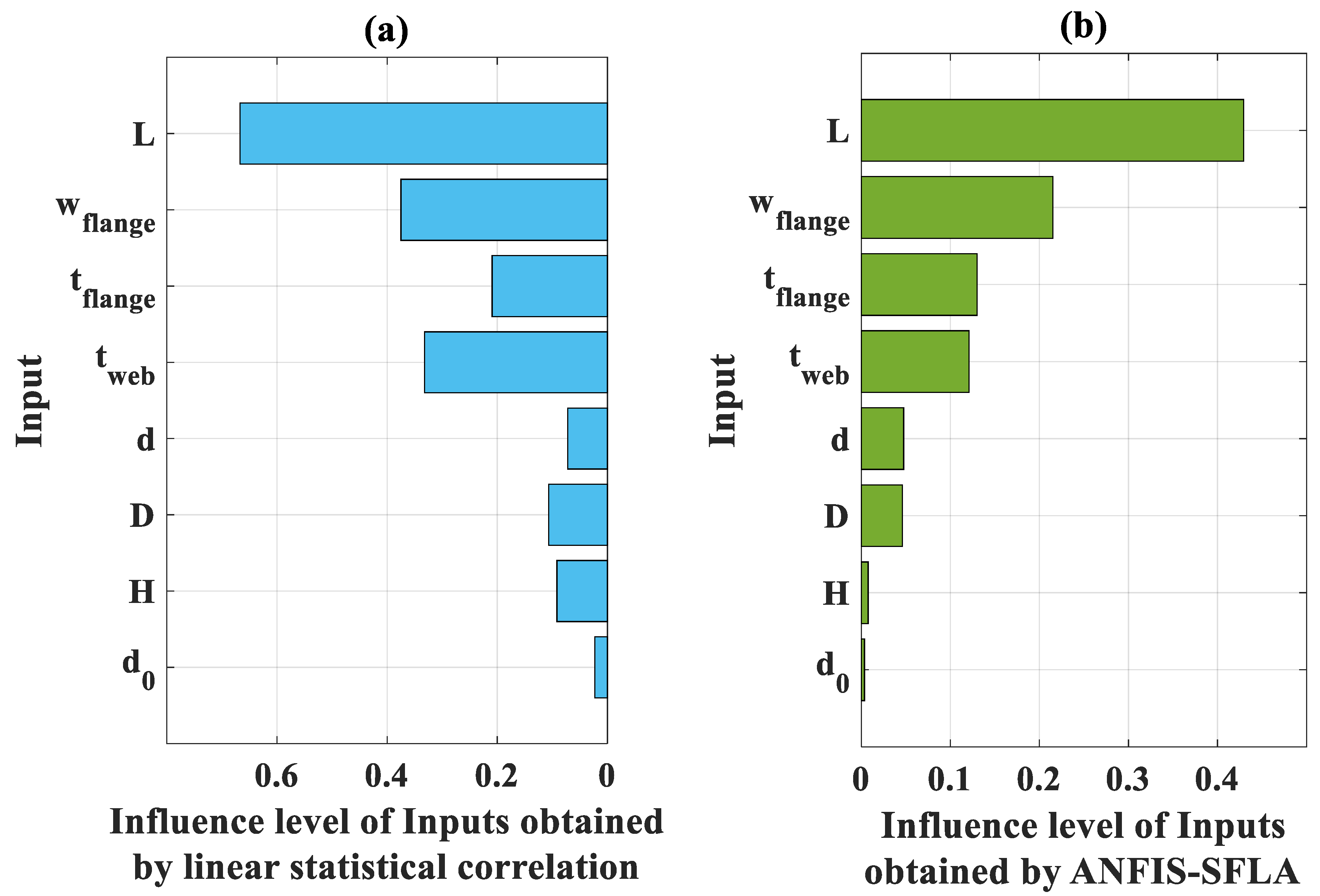
3.3. Sensitivity Analysis

In this section, the sensitivity analysis was performed in favor of quantifying the influence of these inputs to the predicted critical buckling load using the best-found model, namely ANFIS-SFLA. The procedure of the sensitivity analysis is detailed in the following:
A new input space of eight dimensions was constructed based on the probability density function of each variable for evaluating the sensitivity analysis. The new input space composes of only eleven values for each input variable ranging from its smallest to highest quantile with a resolution of 10 (for instance, [0,10,20,30,40,50,60,70,80,90,100]). When calculating the sensitivity for a considered input variable, the values were taken successively from the eleven previously mentioned quantiles, whereas other inputs remained at their median. Therefore, the method obtains information on the deviation of output solution in varying statistically the considered input variable. In this work, the reference case refers to the one where all input variables stayed at their 50% quantile level. For illustration purpose, the more changes on the output solution as compared with the reference case, the more influence the considered input is. Deviation in output solution when evaluating the sensitivity of the jth input variable can be written as the following [48]:
θ i j = Y i j Y r e f Y r e f ,
where Y r e f is the output of the reference case, Y i j is the output solution using jth input at its ith quantile.
Figure 9 shows the evaluation of deviation for eight input variables used in this study. Obviously, all considered input variables govern the buckling capacity of the cellular beam. The critical buckling capacity of the beam decreases when the length, L, and the opening diameter, D, increases, but it increases when the inter-opening distance d, section height H, web thickness tweb, flange width wflange, and flange thickness tflange increase. In addition, the beam end-opening distance, d0, does not significantly affect the buckling capacity of the beam. However, it could be seen that the deviation in output solution is nonlinear in function of input variables, especially L, tweb, tflange, and wflange. In case of the length L, a high order of amplitude is observed as compared with other input variables.
Using the deviation previously presented, the final influence level of each input is calculated by summing all deviations based on the following expression:
Θ j = i = 1 11 | θ i j |
The influence level of all input variables obtained by the ANFIS-SFLA model was scaled into the range of [0, 1] as plotted in Figure 10b. It is seen that the most influenced variable is the beam length L ( Θ L = 0.429 ), following by the flange width wflange ( Θ w flange = 0.215 ), the flange thickness tflange ( Θ t flange = 0.130 ), the web thickness tweb ( Θ t web = 0.121 ), the inter-opening distance d ( Θ d = 0.047 ), the opening diameter D ( Θ D = 0.046 ), the section height H ( Θ H = 0.008 ), and the beam end-opening distance d0 ( Θ d 0 = 0.003 ), respectively.
In parallel, linear statistical correlation between each input and output was also calculated and compared with the results of sensitivity analysis obtained by using ANFIS-SFLA (Figure 10a). It is found that the most dominant relationship with the output is the beam length variable (R = 0.667), followed by the flange width (R = 0.375), web thickness (R = 0.332), flange thickness (R = 0.209), opening diameter (R = 0.107), section height (R = 0.092), inter-opening distance (R = 0.072), and beam end-opening distance (R = 0.023), respectively.
It can be observed that there is a good agreement between the results of the ANFIS-SFLA algorithm with the classical regression approach (Table 7). The classification order of importance obtained by ANFIS-SFLA is also indicated in Table 7. On the basis of the results from ANFIS-SFLA and linear statistical correlation, it can be concluded that the beam length highly affects the critical buckling load of circular openings I-shaped beam, followed by the flange width, flange thickness, and web thickness, respectively.
Overall, without solving complex equations, an approach using hybrid ML models could also indicate these highly nonlinear relationships in an efficient manner and avoid too much computational cost.

4. Conclusions

Accurately predicting the critical buckling load is crucial in the field of structural engineering applications. In this study, different hyrbid ML models, namely ANFIS-RCSA, ANFIS-CA, and ANFIS-SFLA, i.e., a combination of ANFIS with metaheuristic optimization techniques such as RCSA, CA and SFLA, respectively, were used to predict the critical buckling load of I-shaped cellular steel beams with circular openings. A total of 3645 FE configurations on buckling behavior of I-section beams with circular openings were extracted to generate the training and testing datasets. Out of these, a total of eight input variables, namely the beam length, flange width, flange thickness, web thickness, inter-opening distance, opening diameter, section height, and beam end-opening distance, as well as one output variable of the critical buckling load of I-shaped cellular steel beams were used in the modeling. Various validation criteria, namely R, RMSE, and MAE were used to validate and compare the models. In addition, a sensitivity analysis was also done to evaluate the importance of input variables for predicting the critical buckling load of I-shaped cellular steel beams using the ML models.
The results showed that the three hybrid proposed models performed well but ANFIS-SFLA is the best predictor as compared with other models (ANFIS-CA and ANFIS-SFLA). The sensitivity results showed that the length of beam is a dominant factor for predicting the critical buckling load of I-shaped cellular steel beams using the ML models, followed by the flange width, flange thickness, web thickness, inter-opening distance, opening diameter, section height, and the beam end-opening distance, respectively.
Overall, the hybrid ML technique developed in this study offers a powerful tool to accurately predict the critical buckling load of I-shaped cellular steel beams. However, the application of the ML model in engineering practice and design is not often an appropriate way. In further research, the current ANFIS-SFLA prediction function could be exploited to derive an explicit empirical equation for use in practical engineering design and analysis. For this purpose, the sensitivity analysis previously presented could play an important role in deriving the desired formula by searching, first, the empirical coefficients between the output and the most relevant inputs.

Author Contributions

Conceptualization, H.-B.L., T.-T.L., and B.T.P.; methodology, H.-B.L., T.-T.L., and B.T.P.; validation, H.-B.L., T.-T.L., and B.T.P.; formal analysis, H.-B.L., T.-T.L., and B.T.P.; data curation, L.M.L., V.Q.T., V.M.L., H.-L.T.V., and Q.H.N.; writing—original draft preparation, H.-B.L., T.-T.L., L.M.L., V.Q.T., V.M.L., H.-L.T.V., Q.H.N., and B.T.P.; writing—review and editing, H.-B.L., T.-T.L., and B.T.P.; visualization, L.M.L., V.Q.T., V.M.L., H.-L.T.V., and Q.H.N.; supervision, H.-B.L., T.-T.L., and B.T.P.; project administration, H.-B.L.; funding acquisition, T.-T.L.

Funding

This research received no external funding.

Conflicts of Interest

The authors declare no conflicts of interest.

Abbreviation and Nomenclature

SymbolExplanationSI Unit
MLMachine learning
ANFISAdaptive neuro-fuzzy inference system
ANNArtificial neural networks
RCSAReal-coded simulated annealing
CACultural algorithm
SFLAShuffled frog leaping algorithm
RCorrelation coefficient
RMSERoot mean squared error
MAEMean absolute error
StDStandard deviation
Qi (i = 0:100)Quantile value at ith point
LBeam lengthM
d0Beam end-opening distanceMm
DDiameter of circular openingsMm
dInter-opening distanceMm
HHeight of I-sectionMm
twebWeb thicknessMm
wflangeFlange widthMm
tflangeFlange thicknessMm
qUniformly distributed loadN/m
qcCritical buckling loadN/m
mScaling parameter
nScaling parameter

References

  1. Grilo, L.F.; Fakury, R.H.; de Castro e Silva, A.L.R.; de Souza Veríssimo, G. Design procedure for the web-post buckling of steel cellular beams. J. Constr. Steel Res. 2018, 148, 525–541. [Google Scholar] [CrossRef]
  2. Lawson, R.M.; Lam, D.; Aggelopoulos, E.; Hanus, F. Serviceability performance of composite cellular beams with partial shear connection. J. Constr. Steel Res. 2018, 150, 491–504. [Google Scholar] [CrossRef] [Green Version]
  3. Zaher, O.F.; Yossef, N.M.; El-Boghdadi, M.H.; Dabaon, M.A. Structural behaviour of arched steel beams with cellular openings. J. Constr. Steel Res. 2018, 148, 756–767. [Google Scholar] [CrossRef]
  4. Sweedan, A.M.I. Elastic lateral stability of I-shaped cellular steel beams. J. Constr. Steel Res. 2011, 67, 151–163. [Google Scholar] [CrossRef]
  5. Ellobody, E. Nonlinear analysis of cellular steel beams under combined buckling modes. Thin Walled Struct. 2012, 52, 66–79. [Google Scholar] [CrossRef]
  6. Nadjai, A.; Petrou, K.; Han, S.; Ali, F. Performance of unprotected and protected cellular beams in fire conditions. Constr. Build. Mater. 2016, 105, 579–588. [Google Scholar] [CrossRef] [Green Version]
  7. Ly, H.-B.; Desceliers, C.; Le, L.M.; Le, T.-T.; Pham, B.T.; Nguyen-Ngoc, L.; Doan, V.T.; Le, M. Quantification of Uncertainties on the Critical Buckling Load of Columns under Axial Compression with Uncertain Random Materials. Materials 2019, 12, 1828. [Google Scholar] [CrossRef] [Green Version]
  8. Le, L.; Ly, H.-B.; Pham, B.; Le, V.; Phạm, T.; Nguyen, D.-H.; Tran, X.-T.; Le, T.-T. Hybrid Artificial Intelligence Approaches for Predicting Buckling Damage of Steel Columns Under Axial Compression. Materials 2019, 12, 1670. [Google Scholar] [CrossRef] [Green Version]
  9. Ly, H.-B.; Le, L.M.; Duong, H.T.; Nguyen, T.C.; Pham, T.A.; Le, T.-T.; Le, V.M.; Nguyen-Ngoc, L.; Pham, B.T. Hybrid Artificial Intelligence Approaches for Predicting Critical Buckling Load of Structural Members under Compression Considering the Influence of Initial Geometric Imperfections. Appl. Sci. 2019, 9, 2258. [Google Scholar] [CrossRef] [Green Version]
  10. Sonck, D.; Belis, J. Lateral–torsional buckling resistance of cellular beams. J. Constr. Steel Res. 2015, 105, 119–128. [Google Scholar] [CrossRef]
  11. Tsavdaridis, K.D.; D’Mello, C. Web buckling study of the behaviour and strength of perforated steel beams with different novel web opening shapes. J. Constr. Steel Res. 2011, 67, 1605–1620. [Google Scholar] [CrossRef]
  12. Sheehan, T.; Dai, X.; Lam, D.; Aggelopoulos, E.; Lawson, M.; Obiala, R. Experimental study on long spanning composite cellular beam under flexure and shear. J. Constr. Steel Res. 2016, 116, 40–54. [Google Scholar] [CrossRef] [Green Version]
  13. Zainal Abidin, A.R.; Izzuddin, B.A.; Lancaster, F. A meshfree unit-cell method for effective planar analysis of cellular beams. Comput. Struct. 2017, 182, 368–391. [Google Scholar] [CrossRef]
  14. Panedpojaman, P.; Sae-Long, W.; Chub-uppakarn, T. Cellular beam design for resistance to inelastic lateral–torsional buckling. Thin Walled Struct. 2016, 99, 182–194. [Google Scholar] [CrossRef]
  15. Qi, C.; Fourie, A. Cemented paste backfill for mineral tailings management: Review and future perspectives. Miner. Eng. 2019, 144, 106025. [Google Scholar] [CrossRef]
  16. Asteris, P.G.; Kolovos, K.G. Self-compacting concrete strength prediction using surrogate models. Neural Comput. Appl. 2019, 31, 409–424. [Google Scholar] [CrossRef]
  17. Cavaleri, L.; Asteris, P.G.; Psyllaki, P.P.; Douvika, M.G.; Skentou, A.D.; Vaxevanidis, N.M. Prediction of Surface Treatment Effects on the Tribological Performance of Tool Steels Using Artificial Neural Networks. Appl. Sci. 2019, 9, 2788. [Google Scholar] [CrossRef] [Green Version]
  18. Asteris, P.G.; Nikoo, M. Artificial bee colony-based neural network for the prediction of the fundamental period of infilled frame structures. Neural Comput. Appl. 2019, 31, 4837–4847. [Google Scholar] [CrossRef]
  19. Chen, H.; Asteris, P.G.; Jahed Armaghani, D.; Gordan, B.; Pham, B.T. Assessing Dynamic Conditions of the Retaining Wall: Developing Two Hybrid Intelligent Models. Appl. Sci. 2019, 9, 1042. [Google Scholar] [CrossRef] [Green Version]
  20. Reddy, T.C.S. Predicting the strength properties of slurry infiltrated fibrous concrete using artificial neural network. Front. Struct. Civ. Eng. 2018, 12, 490–503. [Google Scholar] [CrossRef]
  21. Waszczyszyn, Z.; Ziemianski, L. Neural networks in mechanics of structures and materials—New results and prospects of applications. Comput. Struct. 2001, 79, 2261–2276. [Google Scholar] [CrossRef]
  22. Le, B.A.; Yvonnet, J.; He, Q.C. Computational homogenization of nonlinear elastic materials using neural networks. Int. J. Numer. Methods Eng. 2015, 104, 1061–1084. [Google Scholar] [CrossRef]
  23. Pham, B.T.; Son, L.H.; Hoang, T.A.; Nguyen, D.M.; Bui, D.T. Prediction of shear strength of soft soil using machine learning methods. Catena 2018, 166, 181–191. [Google Scholar] [CrossRef]
  24. Kopal, I.; Labaj, I.; Harnicarova, M.; Valicek, J.; Hruby, D. Prediction of the Tensile Response of Carbon Black Filled Rubber Blends by Artificial Neural Network. Polymers 2018, 10, 644. [Google Scholar] [CrossRef] [Green Version]
  25. Lefik, M.; Schrefler, B.A. Artificial neural network as an incremental non-linear constitutive model for a finite element code. Comput. Methods Appl. Mech. Eng. 2003, 192, 3265–3283. [Google Scholar] [CrossRef]
  26. Yun, G.J.; Ghaboussi, J.; Elnashai, A.S. A new neural network-based model for hysteretic behavior of materials. Int. J. Numer. Methods Eng. 2008, 73, 447–469. [Google Scholar] [CrossRef]
  27. Qi, C.; Fourie, A.; Chen, Q.; Zhang, Q. A strength prediction model using artificial intelligence for recycling waste tailings as cemented paste backfill. J. Clean. Prod. 2018, 183, 566–578. [Google Scholar] [CrossRef]
  28. Naser, M.Z. Deriving temperature-dependent material models for structural steel through artificial intelligence. Constr. Build. Mater. 2018, 191, 56–68. [Google Scholar] [CrossRef]
  29. Pitton, S.F.; Ricci, S.; Bisagni, C. Buckling optimization of variable stiffness cylindrical shells through artificial intelligence techniques. Compos. Struct. 2019, 230, 111513. [Google Scholar] [CrossRef]
  30. Zhao, Y.; Chen, M.; Yang, F.; Zhang, L.; Fang, D. Optimal design of hierarchical grid-stiffened cylindrical shell structures based on linear buckling and nonlinear collapse analyses. Thin Walled Struct. 2017, 119, 315–323. [Google Scholar] [CrossRef]
  31. Abambres, M.; Rajana, K.; Tsavdaridis, K.D.; Ribeiro, T.P. Neural Network-Based Formula for the Buckling Load Prediction of I-Section Cellular Steel Beams. Computers 2019, 8, 2. [Google Scholar] [CrossRef] [Green Version]
  32. Mallela, U.K.; Upadhyay, A. Buckling load prediction of laminated composite stiffened panels subjected to in-plane shear using artificial neural networks. Thin Walled Struct. 2016, 102, 158–164. [Google Scholar] [CrossRef]
  33. Sadovský, Z.; Guedes Soares, C. Artificial neural network model of the strength of thin rectangular plates with weld induced initial imperfections. Reliab. Eng. Syst. Saf. 2011, 96, 713–717. [Google Scholar] [CrossRef]
  34. Smith, M. ABAQUS/Standard User’s Manual; Version 6.9; Dassault Systemes Simulia Corp: Providence, RI, USA, 2009. [Google Scholar]
  35. El-Sawy, K.M.; Sweedan, A.M.; Martini, M.I. Moment gradient factor of cellular steel beams under inelastic flexure. J. Constr. Steel Res. 2014, 98, 20–34. [Google Scholar] [CrossRef]
  36. Abramovich, H. Stability and Vibrations of Thin-Walled Composite Structures, 1st ed.; Woodhead Publishing: Cambridge, UK, 2017. [Google Scholar]
  37. Ly, H.-B.; Pham, B.T.; Dao, D.V.; Le, V.M.; Le, L.M.; Le, T.-T. Improvement of ANFIS Model for Prediction of Compressive Strength of Manufactured Sand Concrete. Appl. Sci. 2019, 9, 3841. [Google Scholar] [CrossRef] [Green Version]
  38. Nguyen, V.V.; Pham, B.T.; Vu, B.T.; Prakash, I.; Jha, S.; Shahabi, H.; Shirzadi, A.; Ba, D.N.; Kumar, R.; Chatterjee, J.M.; et al. Hybrid Machine Learning Approaches for Landslide Susceptibility Modeling. Forests 2019, 10, 157. [Google Scholar] [CrossRef] [Green Version]
  39. Termeh, S.V.R.; Khosravi, K.; Sartaj, M.; Keesstra, S.D.; Tsai, F.T.-C.; Dijksma, R.; Pham, B.T. Optimization of an adaptive neuro-fuzzy inference system for groundwater potential mapping. Hydrogeol. J. 2019. [Google Scholar] [CrossRef]
  40. Jaafari, A.; Panahi, M.; Pham, B.T.; Shahabi, H.; Bui, D.T.; Rezaie, F.; Lee, S. Meta optimization of an adaptive neuro-fuzzy inference system with grey wolf optimizer and biogeography-based optimization algorithms for spatial prediction of landslide susceptibility. CATENA 2019, 175, 430–445. [Google Scholar] [CrossRef]
  41. Pham, B.T.; Prakash, I. Spatial Prediction of Rainfall Induced Shallow Landslides Using Adaptive-Network-Based Fuzzy Inference System and Particle Swarm Optimization: A Case Study at the Uttarakhand Area, India. In Advances and Applications in Geospatial Technology and Earth Resources; Tien Bui, D., Ngoc Do, A., Bui, H.-B., Hoang, N.-D., Eds.; Springer International Publishing: Basel, Switzerland, 2018; pp. 224–238. [Google Scholar]
  42. Dao, D.; Trinh, S.; Ly, H.-B.; Pham, B. Prediction of Compressive Strength of Geopolymer Concrete Using Entirely Steel Slag Aggregates: Novel Hybrid Artificial Intelligence Approaches. Appl. Sci. 2019, 9, 1113. [Google Scholar] [CrossRef] [Green Version]
  43. Nguyen, H.-L.; Le, T.-H.; Pham, C.-T.; Le, T.-T.; Ho, L.; Le, V.; Pham, B.; Ly, H.-B. Development of Hybrid Artificial Intelligence Approaches and a Support Vector Machine Algorithm for Predicting the Marshall Parameters of Stone Matrix Asphalt. Appl. Sci. 2019, 2019, 3172. [Google Scholar] [CrossRef] [Green Version]
  44. Oonsivilai, A.; El-Hawary, M.E. Power system dynamic load modeling using adaptive-network-based fuzzy inference system. In Proceedings of the Engineering Solutions for the Next Millennium. 1999 IEEE Canadian Conference on Electrical and Computer Engineering (Cat. No.99TH8411), Edmonton, AB, Canada, 9–12 May 1999; Volume 3, pp. 1217–1222. [Google Scholar]
  45. Djukanovic, M.B.; Calovic, M.S.; Vesovic, B.V.; Sobajic, D.J. Neuro-fuzzy controller of low head hydropower plants using adaptive-network based fuzzy inference system. IEEE Trans. Energy Convers. 1997, 12, 375–381. [Google Scholar] [CrossRef]
  46. Nguyen, H.-L.; Pham, B.T.; Son, L.H.; Thang, N.T.; Ly, H.-B.; Le, T.-T.; Ho, L.S.; Le, T.-H.; Tien Bui, D. Adaptive Network Based Fuzzy Inference System with Meta-Heuristic Optimizations for International Roughness Index Prediction. Appl. Sci. 2019, 9, 4715. [Google Scholar] [CrossRef] [Green Version]
  47. Armaghani, D.J.; Hajihassani, M.; Sohaei, H.; Mohamad, E.T.; Marto, A.; Motaghedi, H.; Moghaddam, M.R. Neuro-fuzzy technique to predict air-overpressure induced by blasting. Arab. J. Geosci. 2015, 8, 10937–10950. [Google Scholar] [CrossRef]
  48. Ly, H.-B.; Le, L.M.; Phi, L.V.; Phan, V.-H.; Tran, V.Q.; Pham, B.T.; Le, T.-T.; Derrible, S. Development of an AI Model to Measure Traffic Air Pollution from Multisensor and Weather Data. Sensors 2019, 19, 4941. [Google Scholar] [CrossRef] [Green Version]
  49. Qi, C.; Ly, H.-B.; Chen, Q.; Le, T.-T.; Le, V.M.; Pham, B.T. Flocculation-dewatering prediction of fine mineral tailings using a hybrid machine learning approach. Chemosphere 2019, 244, 125450. [Google Scholar] [CrossRef]
  50. Metropolis, N.; Rosenbluth, A.W.; Rosenbluth, M.N.; Teller, A.H.; Teller, E. Equation of state calculations by fast computing machines. J. Chem. Phys. 1953, 21, 1087–1092. [Google Scholar] [CrossRef] [Green Version]
  51. Kirkpatrick, S., Jr.; Gelatt, C.D.; Vecchi, M.P. Optimization by Simulated Annealing. Science 1983, 220, 671–680. [Google Scholar] [CrossRef]
  52. Černý, V. Thermodynamical approach to the traveling salesman problem: An efficient simulation algorithm. J. Optim. Theory Appl. 1985, 45, 41–51. [Google Scholar] [CrossRef]
  53. Aarts, E.; Korst, J.; Michiels, W. Simulated Annealing. In Search Methodologies: Introductory Tutorials in Optimization and Decision Support Techniques; Burke, E.K., Kendall, G., Eds.; Springer US: Boston, MA, USA, 2005; pp. 187–210. ISBN 978-0-387-28356-2. [Google Scholar]
  54. Zhang, W.; Maleki, A.; Rosen, M.A.; Liu, J. Optimization with a simulated annealing algorithm of a hybrid system for renewable energy including battery and hydrogen storage. Energy 2018, 163, 191–207. [Google Scholar] [CrossRef]
  55. Pham, D.; Karaboga, D. Genetic algorithms, tabu search, simulated annealing and neural networks. In Intelligent Optimisation Techniques; Springer: London, UK, 2000. [Google Scholar]
  56. Dréo, J.; Siarry, P.; Pétrowski, A.; Taillard, E. Metaheuristics for Hard Optimization; Springer: Berlin/Heidelberg, Germany, 2006. [Google Scholar]
  57. Romary, T.; de Fouquet, C.; Malherbe, L. Sampling design for air quality measurement surveys: An optimization approach. Atmos. Environ. 2011, 45, 3613–3620. [Google Scholar] [CrossRef]
  58. Vincent, F.Y.; Redi, A.P.; Hidayat, Y.A.; Wibowo, O.J. A simulated annealing heuristic for the hybrid vehicle routing problem. Appl. Soft Comput. 2017, 53, 119–132. [Google Scholar]
  59. Chung, C.-J. Knowledge-based Approaches to Self-adaptation in Cultural Algorithms. Ph.D. Thesis, Wayne State University, Detroit, MI, USA, 1997. [Google Scholar]
  60. Reynolds, R. An Introduction to Cultural Algorithms; World Scientific Press: Singapore, 1994. [Google Scholar]
  61. Jaafari, A.; Zenner, E.K.; Panahi, M.; Shahabi, H. Hybrid artificial intelligence models based on a neuro-fuzzy system and metaheuristic optimization algorithms for spatial prediction of wildfire probability. Agric. For. Meteorol. 2019, 266–267, 198–207. [Google Scholar] [CrossRef]
  62. Ali, M.Z.; Awad, N.H.; Suganthan, P.N.; Reynolds, R.G. A modified cultural algorithm with a balanced performance for the differential evolution frameworks. Knowl. Based Syst. 2016, 111, 73–86. [Google Scholar] [CrossRef]
  63. Yan, X.; Wu, Q.; Zhang, C.; Chen, W.; Luo, W.; Li, W. An Efficient Function Optimization Algorithm based on Culture Evolution. Comput. Sci. 2012, 9, 11–18. [Google Scholar]
  64. Haldar, V.; Chakraborty, N. Power loss minimization by optimal capacitor placement in radial distribution system using modified cultural algorithm. Int. Trans. Electr. Energy Syst. 2015, 25, 54–71. [Google Scholar] [CrossRef]
  65. Eusuff Muzaffar, M.; Lansey Kevin, E. Optimization of Water Distribution Network Design Using the Shuffled Frog Leaping Algorithm. J. Water Resour. Plan. Manag. 2003, 129, 210–225. [Google Scholar] [CrossRef]
  66. Kennedy, J.; Eberhart, R. Particle swarm optimization. In Proceedings of the ICNN’95—International Conference on Neural Networks, Perth, Australia, 27 November–1 December 1995; Volume 4, pp. 1942–1948. [Google Scholar]
  67. Eusuff, M.; Lansey, K.; Pasha, F. Shuffled frog-leaping algorithm: A memetic meta-heuristic for discrete optimization. Eng. Optim. 2006, 38, 129–154. [Google Scholar] [CrossRef]
  68. Elbeltagi, E.; Hegazy, T.; Grierson, D.E. A modified shuffled frog-leaping optimization algorithm: Applications to project management. Struct. Infrastruct. Eng. 2007, 3, 53–60. [Google Scholar] [CrossRef]
  69. Huynh, T.-H. Duc-Hoang Nguyen Fuzzy controller design using a new shuffled frog leaping algorithm. In Proceedings of the 2009 IEEE International Conference on Industrial Technology, Gippsland, Australia, 10–13 February 2009; pp. 1–6. [Google Scholar]
  70. Jadidoleslam, M. Reliability constrained generation expansion planning by a modified shuffled frog leaping algorithm. Int. J. Electr. Power Energy Syst. 2015, 64, 743–751. [Google Scholar] [CrossRef]
  71. Perez, I.; Gomez-Gonzalez, M.; Jurado, F. Estimation of induction motor parameters using shuffled frog-leaping algorithm. Electr. Eng. 2013, 95, 267–275. [Google Scholar] [CrossRef]
  72. Zhao, Z.; Xu, Q.; Jia, M. Improved shuffled frog leaping algorithm-based BP neural network and its application in bearing early fault diagnosis. Neural Comput. Appl. 2016, 27, 375–385. [Google Scholar] [CrossRef]
  73. Crawford, B.; Soto, R.; Peña, C.; Riquelme-Leiva, M.; Torres-Rojas, C.; Johnson, F.; Paredes, F. Binarization Methods for Shuffled Frog Leaping Algorithms That Solve Set Covering Problems. In Software Engineering in Intelligent Systems; Silhavy, R., Senkerik, R., Oplatkova, Z.K., Prokopova, Z., Silhavy, P., Eds.; Springer International Publishing: Basel, Switzerland, 2015; pp. 317–326. [Google Scholar]
  74. Elbehairy, H.; Elbeltagi, E.; Hegazy, T.; Soudki, K. Comparison of Two Evolutionary Algorithms for Optimization of Bridge Deck Repairs. Comput. Aided Civ. Infrastruct. Eng. 2006, 21, 561–572. [Google Scholar] [CrossRef]
  75. Armaghani, D.J.; Mohamad, E.T.; Narayanasamy, M.S.; Narita, N.; Yagiz, S. Development of hybrid intelligent models for predicting TBM penetration rate in hard rock condition. Tunn. Undergr. Space Technol. 2017, 63, 29–43. [Google Scholar] [CrossRef]
  76. Momeni, E.; Nazir, R.; Armaghani, D.J.; Maizir, H. Application of artificial neural network for predicting shaft and tip resistances of concrete piles. Earth Sci. Res. J. 2015, 19, 85–93. [Google Scholar] [CrossRef]
  77. Dao, D.V.; Ly, H.-B.; Trinh, S.H.; Le, T.-T.; Pham, B.T. Artificial Intelligence Approaches for Prediction of Compressive Strength of Geopolymer Concrete. Materials 2019, 12, 983. [Google Scholar] [CrossRef] [Green Version]
  78. Mohamad, E.T.; Armaghani, D.J.; Momeni, E.; Yazdavar, A.H.; Ebrahimi, M. Rock strength estimation: A PSO-based BP approach. Neural Comput. Appl. 2018, 30, 1635–1646. [Google Scholar] [CrossRef]
  79. Pham, B.T.; Nguyen, M.D.; Bui, K.-T.T.; Prakash, I.; Chapi, K.; Bui, D.T. A novel artificial intelligence approach based on Multi-layer Perceptron Neural Network and Biogeography-based Optimization for predicting coefficient of consolidation of soil. Catena 2019, 173, 302–311. [Google Scholar] [CrossRef]
  80. Zhou, J.; Nekouie, A.; Arslan, C.A.; Pham, B.T.; Hasanipanah, M. Novel approach for forecasting the blast-induced AOp using a hybrid fuzzy system and firefly algorithm. Eng. Comput. 2019. [Google Scholar] [CrossRef]
  81. Khozani, Z.S.; Khosravi, K.; Pham, B.T.; Kløve, B.; Wan Mohtar, W.H.M.; Yaseen, Z.M. Determination of compound channel apparent shear stress: Application of novel data mining models. J. Hydroinform. 2019, 21, 798–811. [Google Scholar] [CrossRef] [Green Version]
  82. Nguyen, M.D.; Pham, B.T.; Tuyen, T.T.; Hai Yen, H.P.; Prakash, I.; Vu, T.T.; Chapi, K.; Shirzadi, A.; Shahabi, H.; Dou, J.; et al. Development of an Artificial Intelligence Approach for Prediction of Consolidation Coefficient of Soft Soil: A Sensitivity Analysis. Open Constr. Build. Technol. J. 2019, 13, 178–188. [Google Scholar] [CrossRef]
  83. Khosravi, K.; Daggupati, P.; Alami, M.T.; Awadh, S.M.; Ghareb, M.I.; Panahi, M.; Pham, B.T.; Rezaie, F.; Qi, C.; Yaseen, Z.M. Meteorological data mining and hybrid data-intelligence models for reference evaporation simulation: A case study in Iraq. Comput. Electron. Agric. 2019, 167, 105041. [Google Scholar] [CrossRef]
  84. Thanh, T.T.M.; Ly, H.-B.; Pham, B.T. A Possibility of AI Application on Mode-choice Prediction of Transport Users in Hanoi. In CIGOS 2019, Innovation for Sustainable Infrastructure; Ha-Minh, C., Dao, D.V., Benboudjema, F., Derrible, S., Huynh, D.V.K., Tang, A.M., Eds.; Springer: Singapore, 2020; pp. 1179–1184. [Google Scholar]
  85. Ly, H.-B.; Monteiro, E.; Le, T.-T.; Le, V.M.; Dal, M.; Regnier, G.; Pham, B.T. Prediction and Sensitivity Analysis of Bubble Dissolution Time in 3D Selective Laser Sintering Using Ensemble Decision Trees. Materials 2019, 12, 1544. [Google Scholar] [CrossRef] [PubMed] [Green Version]
  86. Armaghani, D.J.; Hajihassani, M.; Marto, A.; Faradonbeh, R.S.; Mohamad, E.T. Prediction of blast-induced air overpressure: A hybrid AI-based predictive model. Environ. Monit. Assess. 2015, 187, 666. [Google Scholar] [CrossRef] [PubMed]
  87. Pham, B.T.; Nguyen, M.D.; Dao, D.V.; Prakash, I.; Ly, H.-B.; Le, T.-T.; Ho, L.S.; Nguyen, K.T.; Ngo, T.Q.; Hoang, V.; et al. Development of artificial intelligence models for the prediction of Compression Coefficient of soil: An application of Monte Carlo sensitivity analysis. Sci. Total Environ. 2019, 679, 172–184. [Google Scholar] [CrossRef] [PubMed]
  88. Le, T.-T.; Pham, B.T.; Ly, H.-B.; Shirzadi, A.; Le, L.M. Development of 48-hour Precipitation Forecasting Model using Nonlinear Autoregressive Neural Network. In CIGOS 2019, Innovation for Sustainable Infrastructure; Ha-Minh, C., Dao, D.V., Benboudjema, F., Derrible, S., Huynh, D.V.K., Tang, A.M., Eds.; Springer: Singapore, 2020; pp. 1191–1196. [Google Scholar]
  89. Le, T.T.; Guilleminot, J.; Soize, C. Stochastic continuum modeling of random interphases from atomistic simulations. Application to a polymer nanocomposite. Comput. Methods Appl. Mech. Eng. 2016, 303, 430–449. [Google Scholar] [CrossRef] [Green Version]
  90. Pham, B.T.; Nguyen, M.D.; Ly, H.-B.; Pham, T.A.; Hoang, V.; Van Le, H.; Le, T.-T.; Nguyen, H.Q.; Bui, G.L. Development of Artificial Neural Networks for Prediction of Compression Coefficient of Soft Soil. In CIGOS 2019, Innovation for Sustainable Infrastructure; Ha-Minh, C., Dao, D.V., Benboudjema, F., Derrible, S., Huynh, D.V.K., Tang, A.M., Eds.; Springer: Singapore, 2020; pp. 1167–1172. [Google Scholar]
Figure 1. Schematization of cellular beam under uniformly distributed load.
Applsci 09 05458 g001
Figure 2. Visualization of the FE mesh showing the approximate element size along the span and at the flange surface.
Applsci 09 05458 g002
Figure 3. The joint relationships and histograms between the considered input variables and critical buckling load of the problem (notation is indicated in Table 1).
Applsci 09 05458 g003
Figure 4. Methodology flowchart of this study.
Applsci 09 05458 g004
Figure 5. Optimization costs functions in terms of R using (a) RCSA, (c) CA, and (e) SFLA; in terms of MAE using (b) RCSA, (d) CA, and (f) SFLA.
Applsci 09 05458 g005aApplsci 09 05458 g005b
Figure 6. Graphs of regression between actual and predicted data, for the training dataset using (a) ANFIS-RCSA, (c) ANFIS-CA, and (e) ANFIS-SFLA; for the testing dataset using (b) ANFIS-RCSA, (d) ANFIS-CA, and (f) ANFIS-SFLA.
Applsci 09 05458 g006aApplsci 09 05458 g006b
Figure 7. Graphs of histogram between actual and predicted data for (a) the training dataset and (b) the testing dataset.
Applsci 09 05458 g007
Figure 8. Graphs of error histogram for (a) the training dataset and (b) the testing dataset.
Applsci 09 05458 g008
Figure 9. Evaluation of deviation in output θ (%) for eight input variables, respectively.
Applsci 09 05458 g009
Figure 10. Graphs of sensitivity analysis obtained by (a) linear statistical correlation and (b) ANFIS-SFLA model.
Applsci 09 05458 g010
Table 1. Initial statistical analysis of the dataset.
VariableBeam LengthBeam End-Opening DistanceOpening DiameterInter-Opening DistanceSection HeightWeb ThicknessFlange WidthFlange ThicknessCritical Buckling Load
NotationLd0DdHtwebwflangetflangeqc
UnitmmmmmmmmmmmMmmmN/m
RoleInputInputInputInputInputInputInputInputOutput
Min4.0012.00247.0024.70420.009.00162.0015.0026.40
Q255.00139.50329.0044.80420.009.00162.0015.00100.69
Q506.00256.50373.00108.17560.0012.00216.0020.00169.27
Q757.00370.50448.00162.40700.0015.00270.0025.00289.57
Max8.00718.00560.00274.40700.0015.00270.0025.001361.7
Mean6.00265.36383.56112.51560.0012.00216.0020.00225.68
a StD1.41157.4692.9868.51114.332.4544.104.08182.51
b CV (%)23.5759.3424.2460.9020.4220.4220.4220.4280.87
cm4.0012.00247.0024.70420.009.00162.0015.0026.40
dn8.00718.00560.00274.40700.0015.00270.0025.001361.7
a standard deviation, b coefficient of variation, c scaling parameter, and d scaling parameter.
Table 2. ANFIS’s characteristics.
ParameterValue and Description
Number of inputs8
Number of outputs1
Input membership function typeGaussian
Number of parameters per membership function2
Number of membership function per input10
Output membership function typeLinear
Number of nonlinear parameters160
Number of linear parameters90
Number of total parameters250
Table 3. Parameters of RCSA used in this study.
ParameterValue and Description
Population size50
Initial temperature0.1
Temperature reduction rate0.99
Number of neighbors per individual5
Mutation rate0.5
Mutation standard deviation10%
Stopping iteration1000
Table 4. Parameters of CA used in this study.
ParameterValue and Description
Population size50
Acceptance ratio0.35
Number of accepted individuals18
Stopping iteration1000
Table 5. Parameters of SFLA used in this study.
ParameterValue and Description
Memeplex size50
Number of memeplexes5
Nelder–Mead standard251
Population size1225
Number of parents75
Number of offsprings3
Step size2
Stopping iteration1000
Table 6. Summary of prediction capability.
ModelDatasetRMAERMSEError MeanError StDSlope
ANFIS-RCSATraining0.9270.0320.055−0.0070.0540.749
Testing0.9200.0320.054−0.0060.0540.747
ANFIS-CATraining0.9510.0220.045−0.0050.0450.814
Testing0.9480.0220.044−0.0050.0440.815
ANFIS-SFLATraining0.9620.0170.041−0.0060.0410.822
Testing0.9600.0170.040−0.0060.0400.822
Table 7. Summary of sensitivity analysis.
Input VariableNotationLinear Correlation Coefficient between Variables and TargetInfluence Level Obtained by ANFIS-SFLAClassification Order by ANFIS-SFLA
Beam lengthL0.6670.4291
Beam end-opening distanced00.0230.0038
Opening diameterD0.1070.0466
Inter-opening distanced0.0720.0475
Section heightH0.0920.0087
Web thicknesstweb0.3320.1214
Flange widthwflange0.3750.2152
Flange thicknesstflange0.2090.1303

