Extracting Production Rules for Cerebrovascular Examination Dataset through Mining of Non-Anomalous Association Rules

Abstract

Today, patients generate a massive amount of health records through electronic health records (EHRs). Extracting usable knowledge of patients’ pathological conditions or diagnoses is essential for the reasoning process in rule-based systems to support the process of clinical decision making. Association rule mining is capable of discovering hidden interesting knowledge and relations among attributes in datasets, including medical datasets, yet is more likely to produce many anomalous rules (i.e., subsumption and circular redundancy) depends on the predefined threshold, which lead to logical errors and affects the reasoning process of rule-based systems. Therefore, the challenge is to develop a method to extract concise rule bases and improve the coverage of non-anomalous rule bases, i.e., one that not only reduces anomalous rules but also finds the most comprehensive rules from the dataset. In this study, we generated non-anomalous association rules (NAARs) from a cerebrovascular examination dataset through several steps: obtaining a frequent closed itemset, generating association rule bases, subsumption checking, and circularity checking, to fit production rules (PRs) in rule-based systems. Toward the end, the rule inferencing part was performed by PROLOG to obtain possible conclusions toward a specific query given by a user. The experiment shows that compared with the traditional method, the proposed method eliminated a significant number of anomalous rules while improving computational time.

1. Introduction

Gathering knowledge directly from data (data-driven knowledge) using intelligent data analyses has garnered increasing interest, especially in medical domains, due to their complexity and the large amounts of data available [1]. The growth of observational data, due to the widespread use of electronic health records (EHRs), generates massive amount of medical data storage. Furthermore, extracting hidden usable knowledge of patients’ pathological conditions or diagnoses is essential to supporting the process of clinical decision making and knowledge related to patients’ pathological conditions is also critical for research in the medical domain [2,3,4,5,6,7,8]. Association rule mining (ARM) is one of the common research objectives that generally generates a pattern of disease based on patients’ pathological conditions that are associated by identifying frequent co-occuring item sets from medical data records, depending on the predefined threshold. It describes logical relations with probabilities in the form of an if…then… rule, which is also known as production rules (PRs).

In EHR, each patient is represented by a set of pathological conditions which leads to a wide variation of data in medical dataset because most pathological conditions are usually presented in continuous values. However, physicians prefer discrete terms rather than precise values to find knowledge more appropriate by means of rules and easier to be interpreted. Consequently, due to this discrete form, it is very common to find redundancies in a medical dataset, such as many patients having the same attribute values, which further contributes to the frequency of co-occurrence of the corresponding attribute values in ARM (illustration given in Figure 1). In addition, one might also find inconsistency data when the same set of attributes’ values from one or more data records, e.g., R2 and R4: {age:middle aged, sbp:prehypertension, bmi:acceptable}, belong to different class labels (e.g., mri:normal or mri:abnormal). This kind of data records might require further investigation to ensure which class label is more appropriate to belong to those pathological conditions. Those kind of redundancies may have a negative impact on the quality of clinical documentation and decision making [9,10].

1.1. Relationship between Association Rule Mining (ARM) and Production Rule Systems (PRSs)

There are several gaps between ARM and production rule systems (PRSs). Note that in rule-based systems, the detection of redundant rules is important for several reasons [11]: (1) making a process toward the rules does not have the proper impact if its redundant counterpart remains; (2) rule sets without redundancy often execute more efficiently; and (3) in systems that combine evidence by examining multiple paths to draw a conclusion, redundant rules may lead to irrelevant paths. On the other hand, traditional ARM basically does not consider those drawbacks during the extraction process. The more frequent the co-occurrence of each attribute value in the dataset, the more items can be considered as important item sets to form a set of association rules (ARs). Consequently, a huge number of potential rules will be generated as the number of frequent items increases, because the traditional ARM method considers all possible subsets of frequent item sets as an antecedent part of a rule. Moreover, those rules may still contain structural anomalies, such as subsumption and circular redundancy, which, in PRs, may lead to logical errors and a situation in which no useful information can be shared. No exceptions for rules extracted from medical datasets. These unexpected conditions may also affect the reasoning process of rule-based systems. Therefore, to improve the performance of a production rule system (PRS), the quality of its rule base should be considered and enhanced by handling possible anomalies associated with rule bases [12].

1.2. Anomalies in Rules

There are two types of anomalies that will be discussed in this study: the subsumption redundancy rule and the circular rule. First, a subsumption redundancy rule exists in the present of another rule if two rules conclude the same action, but one has additional constraints in the rule condition, which may or may not be necessary (a specific kind of redundancy). Based on Figure 1, the presence of rule R2 will be considered as redundant subsumption because its antecedent items become the superset of antecedent items in R1 (i.e., age:elderly, sbp:prehypertension ⊇ age:elderly). According to the nature of logical testing in knowledge structure verification, one rule that contains more items in rule condition will be simply discarded without considering whether those rules imply the same knowledge. However, in real-world interpretation, if rule R1 is kept while rule R2 is discarded, then it might be too general to imply that elderly patients are more likely to have abnormality in their MRI brain result, whereas it is possible for R2, which has more items, to be more interesting than one with fewer items in rule condition. If R2 has at least a higher or equal interesting measurement than R1 or another subset of R2 (i.e., sbp:prehypertension→mri: abnormal), then it is obvious that rule R1 is no longer sufficient to represent knowledge of R2. Consequently, eliminating R2 in the presence of R1 may lead to the loss of more interesting knowledge with more constraint information as a rule base. Therefore, taking interestingness measurement into consideration to eliminate redundant rules without losing more useful knowledge is necessary.

Secondly, rules that are extracted from ARM mostly represent relationship between attributes, according to their co-occurrence in the database. Those rules are usually interpreted individually, without considering any relationship between the rules in the set of rules. In contrast, in PRSs, it is possible to deduce new final conclusions by creating a chain and linking two or more rules through a predicate logic approach or rule of inferences. However, it also possible to find another anomaly (i.e., circular condition) during the reasoning process. Circular rules tend to create a closed chain, which restrains the inference process in deducing final conclusions because of its loop. Referring to Figure 1, there is a rule chain R2 → R3 → R4 that contains a circularity which makes the reasoning process enter an endless loop by keeping the insertion of the same facts to the rule base of the production system without making any progress towards the solution or goal of the problem. Therefore, it will be difficult to derive a new final conclusion. Hence, further investigation for circularity reduction is also important in building rule bases to avoid contradictory logic or meanings and endless looping.

1.3. Contributions

Many studies have attempted to extract non-redundant association rules (NRARs) using frequent closed item sets (FCIs) [13,14,15,16] and mining minimal NRARs as an extension of NRAR mining (NRARM) [17,18,19]. Nevertheless, to the best of our knowledge, the generated NRARs may still contain structural anomalies and methods for data-driven knowledge using data mining techniques to obtain non-anomalous rule bases are very limited. The aim of this study was to develop a method to extract a set of concise and anomalous-free PRs for a rule-based system and to improve the efficiency of mining non-anomalous rule bases and also find the most comprehensive rules from the dataset. Therefore, the main contributions of this study are as follows:

• A method, based on NRARs, to support the extraction of rule-based knowledge bases from cerebrovascular examination dataset.
• An additional method to deal with structure anomalies (i.e., subsumption and circular rules) from the extracted NRARs to verify the knowledge through logical testing and finally, a concise non-anomalous knowledge base can be derived for a rule-based system for cerebrovascular examination datasets.
• The proposed method takes a certain factor value [20] of each rule into consideration as it plays important roles in PRs.

The remainder of this paper is organized as follows. The proposed method is presented in Section 2, followed by the Results and Discussion in Section 3 and Section 4, respectively.

2. Method to Extract the Rule-Based Knowledge

The purpose of this study was to investigate how to derive NAARs as concise yet strong PRs to fit rule-based KBs which lead inference systems to successfully make final decisions. By employing the FCI technique, this study proposes a method to extract a set of PRs that satisfy four concise representations, i.e., closed, generator, non-subsumption, and non-circular rules under certainty factor measurements, so-called non-anomalous rules. The initial set of ARs had to satisfy logical testing of knowledge structure verification [21] and become more condensed by finding logical connectives between the rules, as mentioned in [22], before those concise rules were processed through an inference engine to obtain the final conclusion. This study focused on a medical database, especially on cerebrovascular examination data records in Taiwan. Prior to the introduction of our proposed method, some notations and definitions need to be explained.

2.1. Notations and Definitions

According to the application of this study, cerebrovascular examination data records of patients $p=\left\{p1,p2,\dots \right\}$ were collected and denoted as set $D$.

A set of $D=\left\{\left(\left(a_i,{sbp}_i,{bmi}_i,{fg}_i,{tc}_i\right),{mri}_i\right)\right|1\le i\le \left|P\right|\}$ consists of six features: age $\left(a_i\in A\right)$, systolic blood pressure $\left({sbp}_i\in SBP\right)$, body-mass index $\left({bmi}_i\in BMI\right)$, fasting glucose $\left({fg}_i\in FG\right)$, and total cholesterol $\left({tc}_i\in TC\right)$, which correspond to MRI results as class labels $M=\left\{{mri}_1,{mri}_2,\dots \right\}$. Furthermore, there is a collection of distinct items from each feature, denoted $I=\left\{i_1,i_2,\dots \right\}$, thus $A,SBP,BMI,FG,TC\subseteq I$. Set $D$ can be written as $D=\left\{\left(d_i,{mri}_i\right)\right|1\le i\le \left|P\right|\},$ where $d_i=\left(a_i,{sbp}_i,{bmi}_i,{fg}_i,{tc}_i\right)$ for simplicity. Furthermore, one notes that there is no patient with a $BMI$ value in both the obese and underweight ranges at the same time in medical case.

Table 1. An example of a cerebrovascular examination dataset in Taiwan.

PatientID	Age	SBP	MRI_Brain
p1	Adult	Normal	Normal
p2	Elderly	Hypertension I	Abnormal
$⋮$	$⋮$	$⋮$	$⋮$
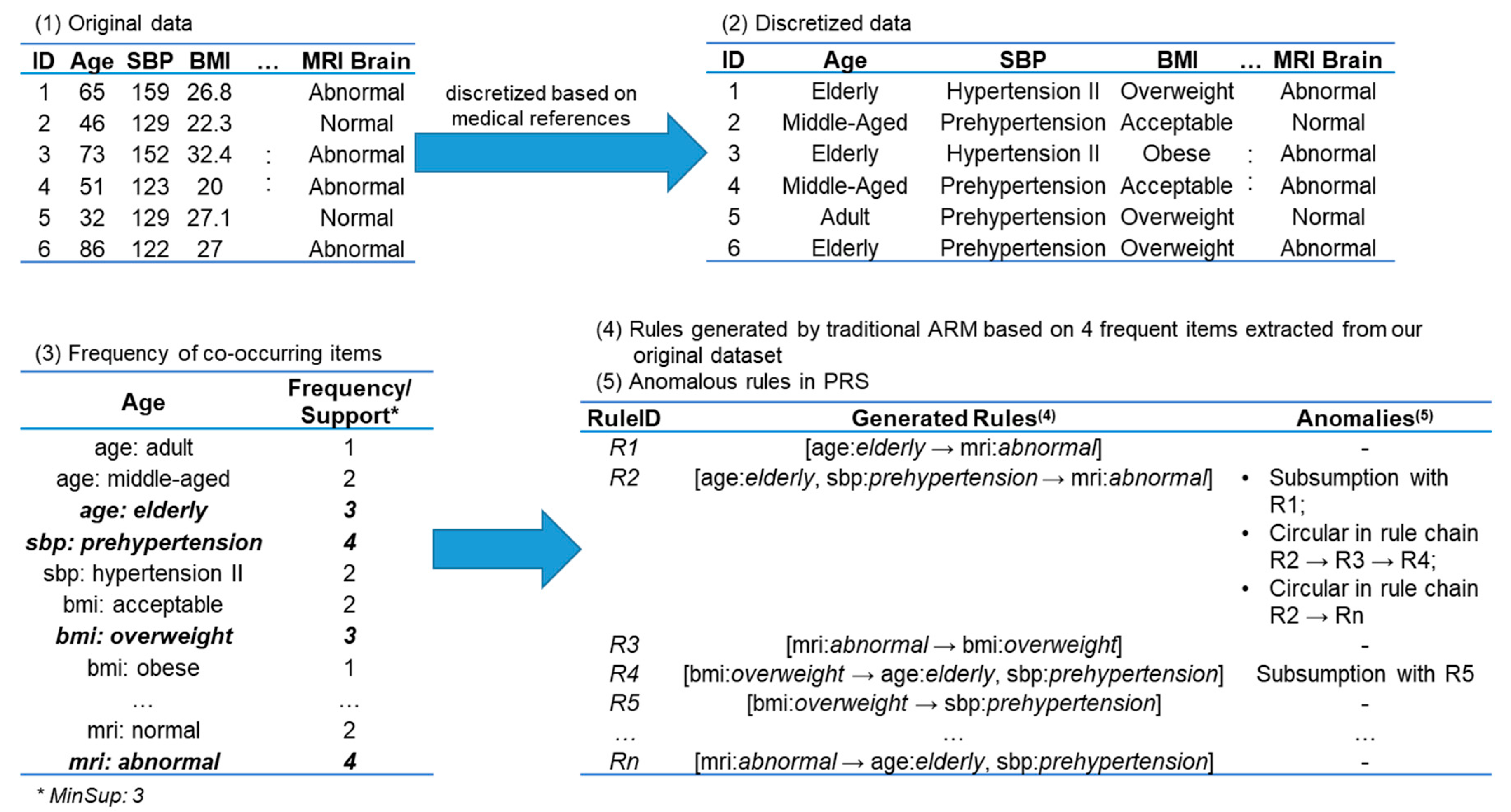
pn	Adolescent	Normal	Normal

gives an illustration of database $D$.

To discover useful information from the database $D$, conventional ARM is a popular data-mining technique to assist experts—i.e., medical practitioners, in this case—in decision making. Useful information can be represented as a rule $ℛ:\left(X\to Y\right)$, where $X,Y\subseteq 1$. Hence, $X$ and $Y$ can also be said to be item sets. To determine an association rule $ℛ$, two measurements need to be defined, e.g., support and confidence values ($sup\left(X\right)$ and $conf\left(X\to Y\right)$, respectively), as follows:

$$sup\left(X\right)=P\left(X\right)=\frac{\left|d\in D;x\subseteq d\right|}{\left|D\right|}$$

(1)

$$conf\left(X\to Y\right)=P\left(Y|X\right)=\frac{sup\left(X\to Y\right)}{sup\left(X\right)}=\frac{\left|d\in D;X\subseteq d,Y\subseteq d\right|}{sup\left(X\right)}$$

(2)

Based on [23], $X$ or $Y$ can be considered a frequent itemset if their support values satisfy a predefined minimum support threshold, $\sigma$, as defined below in Definition 1.

Definition 1.

(Frequent itemset)

Given a minimum support threshold $\sigma \in \left[0,1\right]$, then an itemset $X$ is a frequent itemset if $sup\left(X\right)\ge \sigma$.

In conventional ARM, a generate-and-test approach is employed to collect frequent itemsets and subsequently build ARs based on two predefined threshold values. Formally, conventional ARM is defined as follows.

Definition 2.

(Conventional ARM)

Given minimum support and confidence thresholds $\sigma$ and $\delta \in \left[0,1\right]$, and two frequent itemsets $X$ and $Y$, we extract a set of association rules $ℛ=\left\{\left(Xi\to Yi\right)\right|Xi\in X,Yi\in Y\}$ that fulfill the following conditions:

• $sup\left(Xi\right)\ge \sigma ,\forall Xi\in X$; and
• $conf\left(Xi\to Yi\right)\ge \delta ,\forall Yi\in Y$.

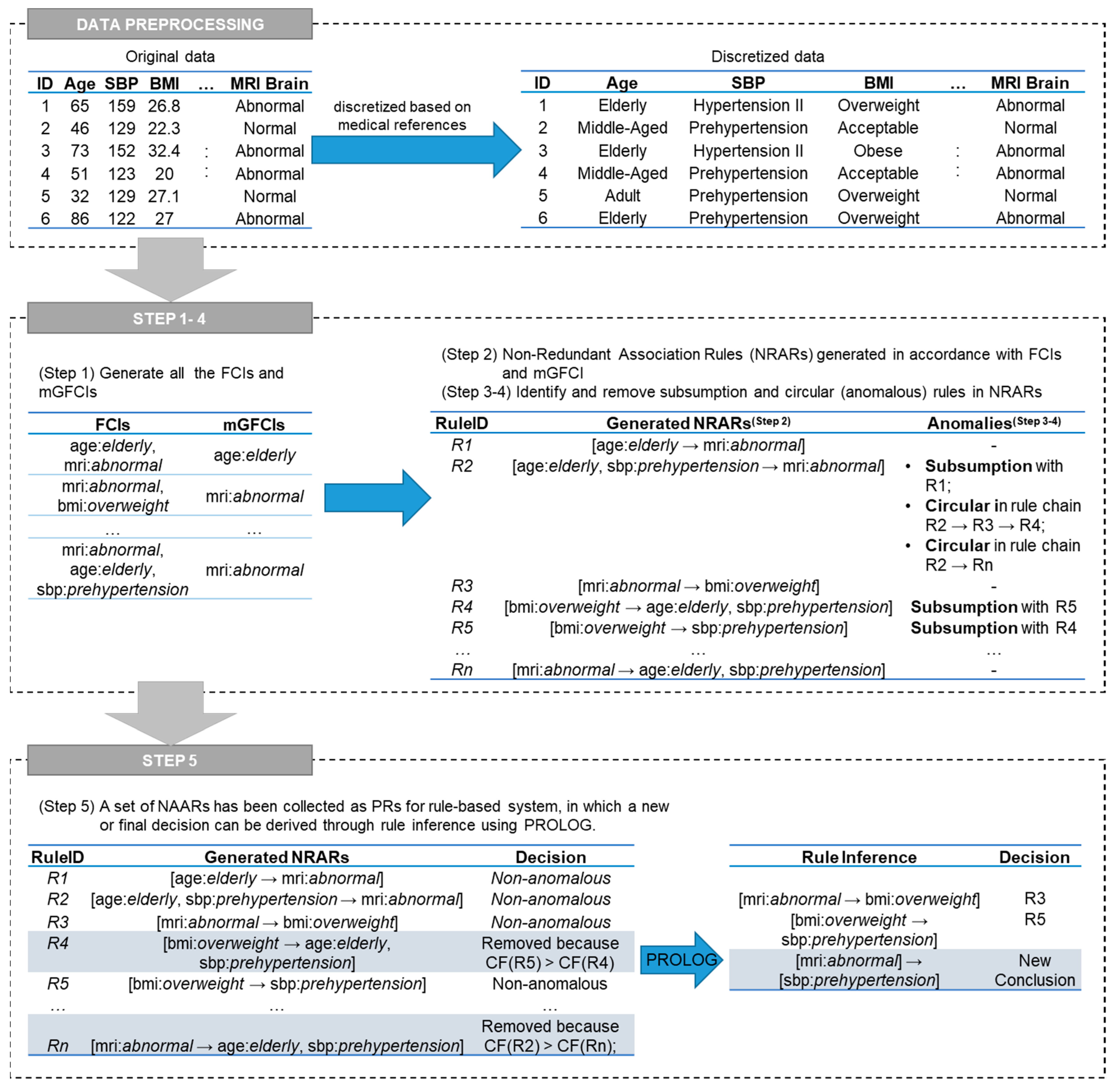
However, conventional ARM is computationally expensive in terms of run-time and memory usage. To overcome this drawback, this study focused on ARM using a hybrid approach [19]—with a vertical database format (the detailed illustration of a vertical format on $D$ is given in Table 3 in Section 2.3.1)—and presents NRARs. Furthermore, there are five types of non-redundant frequent item sets discussed in this study: FCI, generator of FCI (GFCI), minimal GFCI (mGFCI), non-subsumption FCI (nSFCI), and non-circular FCI (nCFCI). Henceforth, this study defines all non-redundant frequent item sets and subsequently generates a set of concise rules, so-called non-anomalous association rules (NAARs), based on the aforementioned types of non-redundant frequent item sets. Moreover, this study also takes some properties of PRs into consideration toward NAARs as the main focus.

An FCI is a frequent itemset which has no superset with the same support values. Formally, an FCI is defined as follows:

Definition 3.

(Frequent Closed Itemset)

Given a frequent itemset $X$, $X$ is an FCI $\iff \nexists Z\ni Z\supseteq X\wedge sup\left(X\right)=sup\left(Z\right)$.

One previous study states that a generator item set should be selected according to the minimum description length [24]. An item set is called a generator if there is no subsequence with the same support values. The formal definition of a generator is presented below.

Definition 4.

(Generator Frequent Closed Itemset)

Given an FCI, where $X$ is a GFCI $\iff \nexists Z\ni X\subseteq Z\wedge sup\left(X\right)=sup\left(Z\right)$.

According to Definition 4, a set of GFCIs may still contain redundant generators, e.g., two GFCIs that share the same information; thus, the longest one can be pruned to enhance the mining process.

Assume we have a set of GFCIs, such that $G=\{\left(a:a1,sbp:sbp2\right),\left(bmi:bmi2,fg:fg1\right),\left(a:a1,bmi:bmi2,sbp:sbp2\right),\left(a:a1,sbp:sbp2,fg:fg1\right),$ $\left(bmi:bmi2,fg:fg1,sbp:sbp1\right)$. After that, we have a set of minimal generators $mG=\left\{\left(a:a1,sbp:sbp2\right),\left(bmi:bmi2,fg:fg1\right)\right\}$, which, by definition, can be described as follows.

Definition 5.

(Minimal Generator Frequent Closed Itemset)

Let $G=\left\{X_{g1},X_{g2},\dots \right\}$ be a set of GFCIs. $X_{g_i}$ can be said to be an mGFCI if $\nexists X_{g_j}\ni X_{g_i}\subseteq X_{g_j}$, where $i=j$ and $X_{g1},X_{g2}\in G$.

Regarding Definition 5, we can clearly state that a set of mGFCIs ($mG$) is not an empty set. Additionally, there is a property of $mG$ as follows.

Property 1.

If$mG$is a set of mGFCIs, then: (i)$mG=\varnothing$; and/or (ii)$mG=G$when no proper generator$X_g\in G$can be found.

By adopting Definition 2, an AR from an mGFCI set can be generated, which is further called a non-redundant association rule (NRAR). In conventional ARM, ARs can be obtained by randomly putting all possible FCIs on the antecedent or consequent sides. However, because the number of mGFCIs is small, it may difficult to construct a rule only from mGFCIs. Conforming to [17], a NRAR can be formed by two combinations between FCIs and mGFCIs. To construct a NRAR, mGFCIs are considered a premise, while items in FCI—excluding that of its corresponding mGFCI—are put as the conclusion. The definition of a NRAR is described below.

Definition 6.

(A Non-Redundant Association Rule)

Let $mG$ be a set of mGFCIs and $F$ is a set of FCIs. A NRAR can be written as $ℛ:X\to \left(Y\backslash X\right)$ where $X\in mG,Y\in F$ and $X\ne Y$.

Regarding Property 1 and Definition 6, we ensure that $Y\backslash X$ is a finite set, which means that we do not need to worry about losing any information, e.g., $\left(X\to \varnothing \right)$. A construction rule, $ℛ:X\to Y$ with $X$, $Y\in F$ and $X=Y$, can still be applied and considered to be a NRAR, even when $mG=F$. On the other hand, since we are trying to obtain concise rule bases, then PRs are also discussed as one of main focuses of this study.

Definition 7.

(Production Rules)

A rule-based mode of knowledge representation is termed a PR. The rule is basically in the form of if <premises> then <conclusions> or similarly if <evidence (E)> then <hypotheses (H)>.

PRs can be applied as rule bases after the collection of rules in PRs is verified through a logical testing procedure. For simplicity, we need to ensure that there is no single rule that can be implied with other rules, called non-subsumption rules (or non-implication rules). For instance, there are two rules:

• ${ℛ}_1:\left(Elderly,sbpisnormal,dbpisHypertensionII\right)\to mri:Abnormal$.
• ${ℛ}_2:\left(Elderly,dbpisHypertensionII\right)\to mri:Abnormal$.

From a physician’s viewpoint, both ${ℛ}_1$ and ${ℛ}_2$ are equivalent rules, since those share similar symptoms, such that $MRI$ result shows $Abnormal$. Hence, a non-subsumption AR can be defined as follows.

Definition 8.

(Non-subsumption ARs)

Suppose there is a set of rules $ℝ$. A rule $ℛ:X\to Y\in ℝ$ is a non-subsumption rule if $\nexists {ℛ}^{*}:X^{*}\to Y^{*}\in ℝ\ni X^{*}\subseteq X,Y^{*}\subseteq Y$.

In addition, both ARs and NRARs may still produce rules in which the conclusion of one rule is the same as the premise of another rule or vice versa. Assume there are two rules:

• ${ℛ}_3:\left(Adolescent,dbpisprehypertension\right)\to mri:Normal$.
• ${ℛ}_4:\left(mri:Normal\right)\to \left(Adolescent,dbpisprehypertension\right)$.

Regarding [21], those rules are considered as a circular rule, which tends to be contradictory in meaning or logic. Hence, ${ℛ}_4$ can be removed. Consequently, rule ${ℛ}_3$ becomes a non-circular rule. The formal definition of non-circular ARs is described below.

Definition 9.

(Non-circular ARs)

Given a set of rules $ℝ$. A rule $ℛ:X\to Y\in ℝ$ is a non-circular rule if $\nexists {ℛ}^{*}:X^{*}\to Y^{*}\in ℝ\ni Y^{*}=X$, i.e., the rules create a closed-chain. In this paper, a rule chain might be formed during rule inference and create a closed-chain (i.e., circularity) in any of the following conditions presented in

Table 2. Type of circularity.

	Type of Circularity	Condition	Definition
1.	DC Type I	$ℛ:X\to Y\in ℝ$ ${ℛ}^{*}:X^{*}\to Y^{*}\in ℝ$	There is a pair of rules $ℛ:X\to Y\in ℝ$ and ${ℛ}^{*}:X^{*}\to Y^{*}\in ℝ\ni Y^{*}=X$
2.	DC Type II	${ℛ}_1:X_1\to Y_1\in ℝ$ $⋮$ ${ℛ}_i:X_i\to Y_i\in ℝ$ $⋮$ ${ℛ}_{n-1}:X_{n-1}\to Y_{n-1}\in ℝ$ ${ℛ}_n:X_n\to Y_n\in ℝ$	There is a rule chain ${ℛ}_1:X_1\to Y_1\in ℝ,\dots ,{ℛ}_n:X_n\to Y_n\in ℝ\ni Y_n=X_{n-1}$
3.	IC Type I	${ℛ}_1:X_1\to Y_1\in ℝ$ $⋮$ ${ℛ}_n:X_n\to Y_n\in ℝ$	${ℛ}_1:X_1\to Y_1\in ℝ,\dots ,{ℛ}_n:X_n\to Y_n\in ℝ\ni Y_n=X_1$
4.	IC Type II	${ℛ}_1:X_1\to Y_1\in ℝ$ $⋮$ ${ℛ}_i:X_i\to Y_i\in ℝ$ $⋮$ ${ℛ}_{n-1}:X_{n-1}\to Y_{n-1}\in ℝ$ ${ℛ}_1:X_n\to Y_n\in ℝ$	There is a rule chain ${ℛ}_1:X_1\to Y_1\in ℝ,\dots ,{ℛ}_n:X_n\to Y_n\in ℝ\ni \exists !X_i=Y_n$ where $i=2,\dots ,n-2$.
Notes:
DC	: Direct-circular
IC	: Indirect-circular

.

Afterwards, a set of NRARs is pruned into NAARs that fulfill both non-subsumption and non-circular rule definitions. In this study, some properties of NAAR mining according to CF values are derived to relate between NAARs and PRs in the following section, then the proposed methodology is introduced.

2.2. NAARs as PRs

This study introduces NAARs that satisfy logical testing in KBs; thus, they can be considered PRs. This paper was motivated by project work in the area of medical diagnoses, called MYCIN, which began in 1972 [20]. It is a rule-based ES for diagnosing infectious blood diseases. MYCIN inferred conclusions from a given condition through certain factor values, which are a calculus of uncertainty for measuring the credibility of a rule, since reasoning in uncertainty is the most important part of MYCIN. Uncertain knowledge representation is also introduced in this PRS by identifying its certainty factor value [25]. As implied, the generation of an AR differs from PRs as there are two quality measurements (i.e., support and confidence) in ARM. However, we found that quality measurements in ARM and PRs share similar statistical-approach concepts, in which Bayesian probability, i.e., conditional probability, is employed. The certainty factor ($CF$) is denoted by

$$CF(ℛ)=\frac{MB\left(Y,X\right)-MD\left(Y,X\right)}{1-\min \left\{MB\left(Y,X\right),MD\left(Y,X\right)\right\}}$$

(3)

where $MB$ is a measurement of belief and $MD$ is a measurement of disbelief which are denoted below.

$$MB\left(Y,X\right)=\{\begin{array}{llll}1& ,\hfill & & P\left(Y\right)=1\hfill \\ \frac{\max \left\{P\left(Y|X\right),P\left(Y\right)\right\}-P\left(Y\right)}{\max \left\{0,1\right\}-P\left(Y\right)}& ,\hfill & & otherwise\hfill \end{array}$$

(4)

$$MD\left(Y,X\right)=\{\begin{array}{llll}1& ,\hfill & & P\left(Y\right)=0\hfill \\ \frac{\min \left\{P\left(Y|X\right),P\left(Y\right)\right\}-P\left(Y\right)}{\min \left\{0,1\right\}-P\left(Y\right)}& ,\hfill & & otherwise\hfill \end{array}$$

(5)

where, $P\left(Y\right)$ is a probability of $Y$ and $P(Y|X)$ is a conditional probability of $Y$ given $X$.

To relate quality measurements in NRARs with $CF$ values in PRs, the gain value of a rule $ℛ$ represents the difference between confidence and support values of an AR, which is denoted as ${Gain}_{AR}(ℛ)$. Later, ${Gain}_{AR}(ℛ)$ can be utilized to relate to $CF(ℛ).$ Based on [26], we show the derivation of ${Gain}_{AR}(ℛ)$.

Lemma 1.

(Gain Value of an AR)

Suppose that $ℛ:X\to Y$ is an AR. The gain value of $ℛ$ is given by

$${Gain}_{AR}(ℛ)=conf(ℛ)-sup\left(Y\right).$$

(6)

Proof. 

$$\begin{array}{c}{Gain}_{AR}(ℛ)=Gain\left(X\to Y\right)\\ \triangleq H\left(Y|X\right)-H\left(Y\right)\\ \approxeq P\left(Y|X\right)-P\left(Y\right)\\ =conf(ℛ)-sup\left(Y\right)\end{array}$$

As in ARM [23], a set of ARs is extracted by satisfying confidence and/or support threshold values, where $sup$ and $conf$ $\in \left[0,1\right]$. Consequently, the range value of ${Gain}_{AR}(ℛ)$ can be determined as a bounded value of $\left[-1,1\right]$.

Corollary 1.

Given an AR$ℛ$, the bounded value of${Gain}_{AR}(ℛ)$is in range$\left[-1,1\right]$.

Proof. 

Since $conf(ℛ)\in \left[0,1\right]$ and $sup\left(Y\right)\in \left[0,1\right]$, $-1\le {Gain}_{AR}(ℛ)\le 0$ when $supp\left(Y\right)=1$, and $0\le {Gain}_{AR}(ℛ)\le 1$ when $conf(ℛ)=1$.

From Equation (6), certainty factors of ARs can be viewed as the ${Gain}_{AR}$ value over the $sup$ value of the consequent part. We denote certainty factor values of ARs as ${CF}_{AR}$. The derivation of ${CF}_{AR}$ is described as follows.

Theorem 1.

(Certainty Factors of ARs)

Let $ℛ:X\to Y$ be an AR. If ${Gain}_{AR}(ℛ)=conf(ℛ)-supp\left(Y\right)$, then we have ${CF}_{AR}(ℛ)\in \left[-1,1\right]$, such that

$${CF}_{AR}(ℛ)=\{\begin{array}{ccc}\frac{{Gain}_{AR}(ℛ)}{1-sup\left(Y\right)},\hfill & & {Gain}_{AR}\left(R\right)\ge 0\\ \frac{{Gain}_{AR}(ℛ)}{sup\left(Y\right)},& & {Gain}_{AR}\left(R\right)<0\end{array}$$

And the range interval of ${CF}_{AR}$ is $\left[-1,1\right]$.

Proof. 

With regard to Corollary 1, it is obvious that ${CF}_{AR}(ℛ)\in \left[-1,1\right]$ as ${Gain}_{AR}(ℛ)\in \left[-1,1\right]$. Hence, there are two main conditions:

• ${Gain}_{AR}(ℛ)\ge 0\iff P(Y|X)\ge P\left(Y\right)$

  $$\begin{array}{c}CF(ℛ)\triangleq \frac{MB\left(Y,X\right)-MD\left(Y,X\right)}{1-\min \left\{MB\left(Y,X\right),MD\left(Y,X\right)\right\}}\\ =\frac{\frac{P\left(Y,X\right)-P\left(Y\right)}{1-P\left(Y\right)}-\frac{P\left(Y\right)-P\left(Y\right)}{P\left(Y\right)}}{1-min\left\{\frac{P\left(Y,X\right)-P\left(Y\right)}{1-P\left(Y\right)},\frac{P\left(Y\right)-P\left(Y\right)}{P\left(Y\right)}\right\}}\\ =\frac{P\left(Y,X\right)-P\left(Y\right)}{1-P\left(Y\right)}\\ =\frac{{Gain}_{AR}(ℛ)}{1-sup\left(Y\right)}\end{array}$$
• ${Gain}_{AR}(ℛ)<0\iff P(Y|X)\ge P\left(Y\right)$

  $$\begin{array}{c}CF(ℛ)\triangleq \frac{MB\left(Y,X\right)-MD\left(Y,X\right)}{1-\min \left\{MB\left(Y,X\right),MD\left(Y,X\right)\right\}}\\ =\frac{\frac{P\left(Y\right)-P\left(Y\right)}{1-P\left(Y\right)}-\frac{P\left(Y,X\right)-P\left(Y\right)}{-P\left(Y\right)}}{1-min\left\{\frac{P\left(Y\right)-P\left(Y\right)}{1-P\left(Y\right)},\frac{P\left(Y,X\right)-P\left(Y\right)}{-P\left(Y\right)}\right\}}\\ =\frac{P\left(Y,X\right)-P\left(Y\right)}{P\left(Y\right)}\\ =\frac{{Gain}_{AR}(ℛ)}{sup\left(Y\right)}\end{array}$$

According to Theorem 1, we can define NAARs, which represent PRs as rule bases. In detail, NRARs, which are still contained of the subsumption or circular rules, are eliminated by considering the smaller ${CF}_{AR}$ value. Considering all the aforementioned discussion, the definition of NAARs in this study is explained as follows.

Definition 10.

(NAARs as PRs)

Let $ℝ=\left\{{ℛ}_1,\dots ,{ℛ}_n\right\}$ be a set of association rules. An association rule ${ℛ}_i=X_i\to Y_i$, with $X_i,Y_i$ are FCI and mGFCI, where $1\le i\le n$, is said to be an NAAR as PR by sequentially satisfying the following conditions:

• $\nexists Z_3\subseteq X$ at this state;
• $\nexists {ℛ}^{*}\in ℝ\ni X^{*}\subseteq X,Y^{*}\subseteq Y$ with ${CF}_{AR}(ℛ)>{CF}_{AR}\left({ℛ}^{*}\right)$; and
• $\nexists {ℛ}^{*}:X^{*}\to Y^{*}\ni Y^{*}=X$ with ${CF}_{AR}(ℛ)>{CF}_{AR}\left({ℛ}^{*}\right)$.

2.3. PR Generation through NAAR Mining and Prolog

This study proposes a method to generate KBs from NRARs that are concise and free from subsumption and circular redundancies. The proposed method contains four main steps and one additional step which is described here.

Step 1.

Generate a set of FCIs and their mGFCIs using the MG-CHARM algorithm [18,19] towards a dataset.

Step 2.

Then, all possible NRARs are constructed based on the FCI and mGFCI set by following Definition 6. Along with this step, the ${CF}_{AR}$ value of each rule must be calculated. At this stage, a set of NRARs can be considered PRs; yet, they still cannot be used as KBs.

Step 3.

In order to consider PRs as KBs, we need to ensure that the PRs have been verified through logical testing, i.e., no subsumption or circular rules. In this step, all subsumption rules in NRARs need to be pruned in accordance with their ${CF}_{AR}$ values. Hence, the remaining NRARs are called non-subsumption NRARs.

Step 4.

Prune all possible circular rules contained in non-subsumptions NRARs to complete logical testing and they can be considered KBs. Henceforth, the final rule set which passed through this stage, is a set of NAARs.

Step 5.

In this step, the rule of the inference process is performed by PROLOG as the prototype of ESs for a cerebrovascular examination dataset. PROLOG answers any query by a user based on KBs obtained from the proposed method.

Basically, Step 1 implements the MG-CHARM algorithm and Step 2 constructs the initial rules with regard to results of the previous step. Thus, we discuss Steps 3 to 5 in more detail in the following section. Additionally, the proposed method also contains a pre-processing step which transforms the original cerebrovascular examination dataset into a dataset with multi-level attributes before mining NRARs. In order to give a better illustration, the framework of the proposed method is depicted in Figure 2.

2.3.1. MineNAAR Algorithm

Since the MG-CHARM algorithm basically uses a vertical transaction format, the cerebrovascular database was transformed into this format. In the horizontal format, the basic form of the dataset is presented as transaction-id in accordance with its item sets. In contrast, in vertical format, the basic form of the dataset is presented in reverse, which means that each item appears in accordance with its transaction-id. An example of the transformation dataset format applied in this study is shown in

Table 3. An example of transformation of the cerebrovascular examination dataset format.

		Item	TID List
		a: a3	2,3
TID	Itemset	a: a5	1
1	a:a5, sdp:sdp1,…, mri:mri2	sdp: sdp1	1,2
2	a:a3, sdp:sdp1, …, mri:mri1	sdp: sdp2	3
3	a:a3, sdp:sdp2, …, mri:mri1	:	:
		mri: mri1	2,3
		mri: mri2	1

.

After the transformation, MG-CHARM was applied to extract all FCIs and mGFCIs in the cerebrovascular examination dataset. Then, concise redundant rules were generated based on the collection of mGFCIs and their corresponding FCIs, which were further put into post-pruning procedures until a set of NAARs was generated. To obtain a set of NAARs, this study introduces an algorithm called MineNAAR which contains four main stages: (1) discovering FCIs and mGFCIs; (2) generating a set of NRARs; (3) pruning subsumption rules; and (4) extracting non-circular rules. Mining PRs from the NRAR set is non-trivial. As we explained above, ARs can be considered as PRs by pruning all rules that are anomalous, i.e., those that still contain subsumption or circular errors. This study also investigated some properties to reduce anomalies, which are contained in NRARs. The MineNAAR algorithm is described in Algorithm 1.

Algorithm 1 NAARs Mining
	Input: A cerebrovascular database $D$, a distinct itemset $I$, minimum support threshold $\sigma$, and minimum confidence threshold $\delta$. Output: $ℝ$ is a set of NAARs.
1:	procedure MineNAAR $\left(D,I,\delta ,\sigma \right)$
2:	${\mathit{ℛ}}_{car}=\varnothing$;
3:	$\left\{\mathit{F},\mathit{m}\mathit{G}\right\}=MGCHARM\left(D,I,\sigma \right)$;
4:	for all ${mG}_i\in \mathit{m}\mathit{G}$ do
5:	for all $g\in {mG}_i\ni g\ne f,f\in \mathit{F}$ do
6:	${\mathit{ℛ}}_{car}={\mathit{ℛ}}_{car}\cup \left\{g\to f\backslash g,f·sup\right\}$;
7:	Compute ${CF}_{AR}\left({ℛ}_{car}\right)$ in $D$;
8:	end for
9:	end for
10:	${\mathit{ℛ}}_{sub}=$ SubsumptionCheck $\left({\mathit{ℛ}}_{car},{CF}_{AR},D\right)$;
11:	${\mathit{ℛ}}_{cir}=$ CircularCheck $\left({\mathit{ℛ}}_{sub},{CF}_{AR},D\right)$;
12:	$ℝ={\mathit{ℛ}}_{cir}$;
13:	end procedure.

The first problem in MineNAAR is to remove all subsumption rules from a set of NRARs based on Definition 8. There are two main cases to reduce subsumption rules based on ${CF}_{AR}$ values. A property to deal with subsumption rules is described as follows.

Property 2.

If there are two NRARs${ℛ}_1:X_1\to Y_1$and${ℛ}_2:X_2\to Y_2$, which are considered to be subsumption rules according to Definition 8, then:

• A NRAR can be pruned when the ${CF}_{AR}$ value of one rule is lower than that of another rule;
• A NRAR with a larger number of items in the antecedent part can be removed when $Y_1=Y_2$ and ${CF}_{AR}\left({ℛ}_1\right)={CF}_{AR}\left({ℛ}_2\right)$; and
• A NRAR with a smaller number of items in the consequent part can be pruned when $X_1=X_2$ and ${CF}_{AR}\left({ℛ}_1\right)={CF}_{AR}\left({ℛ}_2\right)$.

Based on Property 2, an algorithm to prune all subsumption rules is presented as SubsumptionCheck in Algorithm 2.

Algorithm 2 Building Non-subsumption Rules
	Input: A set of concise association rules ${\mathit{ℛ}}_{car}$, $CF$ values of ${\mathit{ℛ}}_{car}$, a cerebrovascular database $D$. Output: ${\mathit{ℛ}}_{sub}$ is a set of non-subsumption NRARs.
1:	procedure SubsumptionCheck $\left({\mathit{ℛ}}_{car},{CF}_{AR},D\right)$
2:	for each ${\mathit{ℛ}}_i\in {\mathit{ℛ}}_{car}$ do
3:	for each ${\mathit{ℛ}}_j\in {\mathit{ℛ}}_{car},i=j$ do
4:	if $X_i=X_j$ or $Y_i=Y_j$ then
5:	if ${CF}_{AR}\left({ℛ}_i\right)={CF}_{AR}\left({ℛ}_j\right)$ then
6:	delete ${\mathit{ℛ}}_i/{\mathit{ℛ}}_j$ which has the lower ${CF}_{AR}$;
7:	else
8:	if $X_i=X_j$ then
9:	delete ${\mathit{ℛ}}_i/{\mathit{ℛ}}_j$ which has more items in antecedent
10:	from ${\mathit{ℛ}}_{car}$;
11:	else if $Y_i=Y_j$ then
12:	delete ${\mathit{ℛ}}_i/{\mathit{ℛ}}_j$ which has least items in consequent
13:	from ${\mathit{ℛ}}_{car}$;
14:	end if
15:	end if
16:	end if
17:	end for
18:	end for
19:	${\mathit{ℛ}}_{sub}={\mathit{ℛ}}_{car}$
20:	end procedure.

The second problem is to avoid circular rules regarding Definition 9 from the generated non-subsumption NRARs. To overcome this problem, all of the non-subsumption NRARs are sorted in descending order of certainty factor values. Furthermore, there are several circularity conditions that must be considered as described in Table 2.

Property 3.

If there are three NRARs${ℛ}_1:X_1\to Y_1$,${ℛ}_2:X_2\to Y_2$, and${ℛ}_3:X_3\to Y_3$which are considered to be circular rules regarding Definition 9, then,

• Remove a rule that has a lower $CF$ value when a rule chain forms any of the direct-circular (DC) conditions.
• If some rules are linked and creating a rule-chain in a way of any of the indirect-circular (IC) conditions, then remove the last rule in the rule-chain.

An algorithm is introduced called CircularCheck to implement Property 3. After the non-subsumption rules from Algorithm 2, CircularCheck is applied to obtain NAARs. In addition, CircularCheck is described in Algorithm 3. The last algorithm results in non-circular and non-subsumption NRARs. For simplicity, we call these NAARs.

Algorithm 3 Building Non-circular Rules
	Input: A set of non-subsumption ARs ${\mathit{ℛ}}_{sub}$, $CF$ values of ${\mathit{ℛ}}_{sub}$, a cerebrovascular database $D$. Output: ${\mathit{ℛ}}_{cir}$ is a set of non-circular NRARs.
1:	procedure CircularCheck $\left({\mathit{ℛ}}_{sub},{CF}_{AR},D\right)$
2:	${\mathit{ℛ}}_{temp}=\varnothing$
3:	for each ${\mathit{ℛ}}_i\in {\mathit{ℛ}}_{sub}$ do
4:	for each ${\mathit{ℛ}}_j\in {\mathit{ℛ}}_{sub}\backslash {\mathit{ℛ}}_i,i=j$ do
5:	if $X_i=Y_j$ and $Y_i=X_j$ then
6:	if ${CF}_{AR}\left({ℛ}_i\right)>{CF}_{AR}\left({ℛ}_j\right)$ then
7:	${\mathit{ℛ}}_{sub}={\mathit{ℛ}}_{sub}\backslash {\mathit{ℛ}}_j$;
8:	else if ${CF}_{AR}\left({\mathit{ℛ}}_i\right)<{CF}_{AR}\left({\mathit{ℛ}}_j\right)$ then
9:	${\mathit{ℛ}}_{sub}={\mathit{ℛ}}_{sub}\backslash {\mathit{ℛ}}_i$;
10:	end if
11:	else if $Y_i=X_j$ then
12:	while $Y_j\ne X_i$
13:	for each ${\mathit{ℛ}}_{j+1}\in {\mathit{ℛ}}_{sub}\backslash ({\mathit{ℛ}}_i\wedge {\mathit{ℛ}}_j),j=j+1$ do
14:	${\mathit{ℛ}}_{temp}={\mathit{ℛ}}_{temp}\cup \left(X_i\to Y_j\right)$;
15:	end for
16:	end while
17:	if $X_{j-1}=Y_j$ and $Y_{j-1}=X_j$ then
18:	if ${CF}_{AR}\left({ℛ}_{j-1}\right)>{CF}_{AR}\left({ℛ}_j\right)$ then
19:	${\mathit{ℛ}}_{sub}={\mathit{ℛ}}_{sub}\backslash {\mathit{ℛ}}_j$;
20:	else if ${CF}_{AR}\left({ℛ}_i\right)<{CF}_{AR}\left({ℛ}_j\right)$ then
21:	${\mathit{ℛ}}_{sub}={\mathit{ℛ}}_{sub}\backslash {\mathit{ℛ}}_{j-1}$;
22:	end if
23:	else if $X_i=Y_j$ or $\exists !X_i=Y_j$ where $i=2,\dots ,j-2$ then
24:	${\mathit{ℛ}}_{sub}={\mathit{ℛ}}_{sub}\backslash {\mathit{ℛ}}_j$;
25:	end if
26:	end if
27:	end for
28:	end for
29:	${\mathit{ℛ}}_{cir}={\mathit{ℛ}}_{sub}$;
30:	end procedure.

2.3.2. Rule Inference Using Prolog

A set of NAARs can simply put on Prolog to inference rules and obtain conclusions in accordance with PRs that we have obtained. Those NAARs are treated as facts in rule-based systems. In PRSs, note that it is possible to deduce new final conclusions by creating a chain and linking two or more rules through a predicate logic approach or rule of inferences as long as the rule chain is non-circular. For instance, suppose we have three NAARs: $R_1:X_1\to Y_1$, $R_2:X_2\to Y_2$ and $R_3:X_3\to Y_3$. Thus, we can create a rule-chain, $R_1\to R_2\to R_3$, from those rules as long as $Y_1=X_2,Y_2=X_3$ and $Y_3\ne X_1$. According to predicate logic, we can deduce a new conclusion, $R_1:X_1\to Y_3$, from the rule-chain based on the concept of hypothetical syllogism by creating the Prolog rule format to make conditional statements about our rule bases clear for programming the inference engine.

Example 1.

 

Suppose we have two rules which create a rule chain:

${ℛ}_1:\left(bmi:obese\right)\to \left(sbp:hypertension1\right)$.

${ℛ}_2:\left(sbp:hypertension1\right)\to \left(mri:abnormal\right)$.

Then, $bmi$ is the attribute and $obese$ is the value. An attribute-value pair will look like av(Attribute, Value);

where Attribute and Value are simple atoms. Then, the fact structure in Prolog looks like rule(LHS, RHS).

rule(lhs([av(bmi,obese)]), rhs(av(sdp,hypertension_I))).

rule(lhs([av(sdp,hypertension_I)]), rhs(av(mri_brain,abnormal))).

While the conclusion deduced for a rule-chain can be inferred through hypothetical syllogism logic, as represented by the following Prolog rule format:

Conclusion(X,Z):-rule(X, Y), rule(Y, Z).

3. Results and Discussion

As mentioned in Section 1, we proposed a method to extract a set of concise and anomalous-free PRs for rule-based system from mining NAARs and also find the most comprehensive rules from the dataset so that those rules can be used as rule-based knowledge to obtain final conclusions through an inference engine. In knowledge-based system engineering, verification of the knowledge is the process of ensuring its quality. Verification of the knowledge was computed inside the proposed method to extract a set of NAARs by detecting redundancies or anomalies among the generated rules and eliminate them in accordance with certainty factor measurements to ensure the reliability of the PRs. Consequently, the extracted NAARs are used as PRs (facts) for the inference engine.

3.1. Performance Comparison

All of the experiments in this paper were executed in MATLAB R2014a on a personal computer running a Windows Operating System with an Intel Core i5 processor, 4 GB of RAM, and a clock speed of 3.40 GHz. For evaluation purposes, the performance results of mining NAARs are for the following objectives: (1) rate of anomalies; (2) number of final rules; (3) processing time. We compared our proposed method in several scenarios (i.e., reduce only circular rules (CR), reduce only subsumption rules (SR), and reduce both anomalous rules (AR)) with the traditional method, the results of which are shown in Figure 3 and Figure 4.

Figure 3 depicts a comparison of level of anomalies and the total number of final rules generated, with different support threshold values. It can be observed that the number of final rules from the traditional method increased significantly as the support threshold decreased. The proposed method could generate a four to five times lower number of rules compared with the traditional method. This condition occurred because of the nature of traditional method which consider all possible combination of items to generate rules. Moreover, considering all the possible combination of items might lead to an increased number of redundancies or anomalies contained in those rule sets. Therefore, as shown in Figure 3, it also produces the highest level of anomalies, which reaches around twice the anomalous rate of those rules produced by the proposed method. On the other hand, in our proposed method, we verify each of the extracted rules with respect to a set of rules which contains all possible subsets or superset of the corresponding rule to be verified in order to find anomalous rules. Hence, the proposed method produces fewer rules. In addition, the level of anomalies reduces with the increase of support values because at a higher support threshold, the total number of generated rules also decreases and leads to fewer potential anomalous rules being found.

In addition, the difference of total number of rules after reducing only circularity only between the traditional and proposed-CR is not huge, yet may still contain subsumption rules. Meanwhile, proposed-SR shows that there are more rules being reduced due to subsumption rules which created a significant difference number of final rules generated with the traditional method. However, similarly to the proposed-CR, it might still contain another anomaly (i.e., circular rules). Therefore, it is better to reduce all possible anomalies, such as the proposed-AR. In comparison with our proposed approach (i.e., proposed-AR), one can see that the total number of rules generated decreases drastically compared with the traditional approach since it removes both anomalies: subsumption and circular rules, in which subsumption rules contribute more in level of anomalous than circular rules.

As mentioned above, since the traditional method considers all possible combinations of items to generate rules, it is obvious that in terms of processing time, the traditional method will take a significantly longer time than the proposed approach. In contrary, our proposed method generates rules based on a depth-first search method and a closed framework, thus, not all possible combinations of item sets will be traversed and evaluated. Therefore, the proposed method could trim searching time and generate rules more efficiently. According to Figure 4, it seems that proposed-SR computation time is the lowest. However, note that our proposed-AR considers both anomalies to be found, while the proposed-SR only reduces subsumption reduction regardless the existence of possible circular rules. Thus, the former took a slightly longer time than proposed-SR. Toward the end, we can conclude that our proposed method could generate concise and less anomalous rules than the traditional approach with relatively more efficient in processing time.

3.2. Subsumption Checking

The proposed method provides clear and understandable information about the inconsistencies found in the rule-base and verifies every rule with another set of rules to find redundancies. To ensure that the extracted PRs is consistent, this study focused on reducing subsumption and circular rules. Regarding [27], the proper rule and its corresponding sub-antecedent have the same consequent itemset, while the proper rule and its corresponding sub-consequent have the same antecedent itemset. In these conditions, a proper rule might have subset items in other rules, which can lead to the occurrence of redundant rules. Hence, it is necessary to eliminate either the proper rule or its corresponding sub-antecedent/consequent when the certainty factor of one rule is higher than the other.

For instance,

Table 4. Example of subsumption rules (proper rule and its sub-antecedents) (1).

Rule ID	Antecedent	Consequent	CF
14	A: Elderly	MRI: Abnormal	0.631	sub-antecedent
90	[A: Elderly ˄ SBP: Prehypertension]	MRI: Abnormal	0.593	sub-antecedent
134	[A: Elderly ˄ TC: Normal]	MRI: Abnormal	0.662	sub-antecedent
350	[A: Elderly ˄ SBP: Prehypertension ˄ TC: Normal]	MRI: Abnormal	0.722	proper rule
Notes:
A	: Age
SBP	: Systolic Blood Pressure
TC	: Total Cholesterol
MRI	: Magnetic Resonance Imaging

shows an example of subsumption rules detected by rule IDs 14, 90, 134, and 350 which contained subset items of its proper rule (rule 350) and have the same consequent item set $\left(mri:Abnormal\right)$. Regarding certainty factor values of the rules shown in the table, we can see that all the rules in the sub-antecedent group are lower that its proper rule. This implies that a single proper rule (rule 350) is sufficient to express the knowledge or the meaning of the three sub-antecedent rules. Therefore, the proper rule is more comprehensive than its sub-antecedent rules. In other words, the proper rule could allow the support and improvement of the diagnosis of abnormal MRI result when more conditions are known, such as shown in rule 350: an elderly patient with prehypertension level of systolic and normal total cholesterol level, rather than each of those sub-antecedent conditions appears alone to diagnose MRI result ‘abnormal’. The proper rule could represent better knowledge with a quite high positive dependency between the conditions presented in the antecedent part and its consequent part indicated by certainty factor value of around 72%, which is also the highest amongst its possible sub-antecedent rules.

Another example can be seen in

Table 5. Example of subsumption rules (proper rule and its sub-consequences).

Rule ID	Antecedent	Consequent	CF
45	[TC: High Cholesterol ˄ SBP:Normal]	A: Middle Aged	0.453	sub-consequent
46	[TC: High Cholesterol ˄ SBP:Normal]	FG: Normal	0.484	sub-consequent
315	[TC: High Cholesterol ˄ SBP:Normal]	[A: Middle Aged ˄ MRI: Abnormal]	0.177	sub-consequent
319	[TC: High Cholesterol ˄ SBP:Normal]	[FG: Normal ˄ MRI: Abnormal]	0.168	sub-consequent
321	[TC: High Cholesterol ˄ SBP:Normal]	[A: Middle Aged ˄ FG: Normal]	0.375	sub-consequent
846	[TC: High Cholesterol ˄ SBP:Normal]	[A: Middle Aged ˄ FG: Normal ˄ MRI: Abnormal]	0.164	proper rule
Notes:
A	: Age
SBP	: Systolic Blood Pressure
TC	: Total Cholesterol
FG	: Fasting Glucose
MRI	: Magnetic Resonance Imaging

, which shows that the program detected that rules 45, 46, 315, 319, 321, and 846 are subsumption. Rule 846 is basically the proper rule and rules 46, 315, 319, and 321 are its sub-consequences because they have the same antecedent items, but the items in their consequent part are a subset of the consequent part of the proper rule. In the case of subsumption redundancy rules, Table 5 shows that all sub-consequence rules have higher CF values than its corresponding proper rule. Since sub-consequence rules imply the same meaning as the proper rule, the proper rule 846 is considered to be redundant in the presence of its sub-consequence rules. Consequently, sub-consequence rules are retained and re-evaluated with the other rules while the proper rule is discarded. Different from the previous instance, the proper rule shown in Table 5 holds the least certainty factor value, around 16.4%, in comparison with its possible sub-consequent rules found in the generated rules.

This example of Table 5 implies that rather than to support the diagnosis of abnormal MRI result for a middle age patient with normal fasting glucose level all together, someone with a high cholesterol level and normal systolic blood pressure is more likely to support several possible subsets of items in consequent part from its proper rule (rule 846), e.g., sub-consequent rule 315: a middle age patient with abnormal MRI result. This means that the proper rule is still insufficient to replace the knowledge contained in its sub-consequent rules into a single rule. Although its CF value is only slightly higher than its proper rule, around 17.7%, the antecedent part of rule 315 still has better representation of positive dependency toward its consequent part. Moreover, by keeping sub-consequent rule 315, it might still contribute to be a consideration of another proper rules as sub-antecedence or sub-consequence or even become the proper rule of another set of sub-antecedence or sub-consequence rules in the next iteration.

On the other hand, another example scenario that can occur during subsumption checking is presented in

Table 6. Example of subsumption rules (proper rule and its sub-antecedents) (2).

Rule ID	Antecedent	Consequent	CF
33	SBP: Normal	FG: Normal	0.298	sub-antecedent
46	[TC: High Cholesterol ˄ SBP: Normal]	FG: Normal	0.484	sub-antecedent
277	[BMI: Overweight ˄ SBP: Normal]	FG: Normal	0.119	sub-antecedent
307	[TC: High Cholesterol ˄ BMI: Overweight ˄ SBP: Normal]	FG: Normal	0.542	sub-antecedent
837	[TC: High Cholesterol ˄ BMI: Overweight ˄ SBP: Normal ˄ A: Middle Aged]	FG: Normal	0.431	proper rule
Notes:
A	: Age
SBP	: Systolic Blood Pressure
BMI	: Body Mass Index
FG	: Fasting Glucose
TC	: Total Cholesterol

. In this case, one can see that among all of the obtained sub-antecedent rules of the proper rule (rule 837) only two sub-antecedent rules (rules 46 and 307) have a higher CF value compared to the proper rule. Since the proper rule still has sub-antecedent rules which are more interesting, we cannot imply that the proper rule can express the same meaning in the presence of rules 46 and 307 (i.e., some of the sub-antecedent rules). Hence, in this case, the proper rule is considered to be the redundant rule and should be discarded from the rule database while all of the sub-antecedent rule group is retained for further checking.

A similar condition to Table 6 can also be seen in

Table 7. Example of subsumption rules (proper rule and its sub-consequences) (2).

Rule ID	Antecedent	Consequent	CF
677	[FG: Diabetes ˄ BMI: Overweight ˄ MRI: Normal]	TC: Normal	0.101	sub-consequent
680	[FG: Diabetes ˄ BMI: Overweight ˄ MRI: Normal]	A: Middle Aged	0.428	sub-consequent
1044	[FG: Diabetes ˄ BMI: Overweight ˄ MRI: Normal]	[A: Middle Aged ˄ TC: Normal]	0.192	proper rule

, where, among all of the obtained sub-consequent rules of the proper rule (rule 1044), there is one sub-consequent rule (rule 680) that has a higher CF value compared to the proper rule. In this condition, we also cannot imply that the proper rule represents the same meaning as its sub-consequent rules because at least one sub-consequent rule occurs that is more interesting than the proper rule. Therefore, we should keep the sub-consequent rule group for further evaluation and eliminate the redundant rule (i.e., the proper rule).

Towards this end, as shown in Figure 5, the result from our proposed algorithm shows that it can detect 1026 subsumption rules from an initial set of 1295 extracted rules. The proposed method reduced a greater number of redundant rules because the total number of extracted rules grew and led to a greater number of redundant rules when the support threshold was low. Moreover, from the abovementioned instances from the experiment, we could see that rules must be analyzed not only based on the number of items contained in the rule’s antecedent or consequent, but also considering the interestingness measure of each rule before deciding which rule is to be considered as anomalous and discarded.

3.3. Circularity Checking

After performing subsumption checking, the current rules are subjected to circularity checking. Basically, there are two type of circularity in this study, as previously mentioned in Definition 9. In the case of direct-circular rules, the program detected 54 conditions of direct-circular rules, which basically contained 27 pairs of direct-circular rule conditions. The following table contains examples of direct-circular rules that were detected. In KBSs when there is a circular redundancy in the rule base, then the last rule of the cycle can simply be eliminated. In the direct-circular type I scenario, even though the order of the circular rules is swapped, they maintain their circularity. For instance, in

Table 8. Example result of direct-circular type I.

Rule ID	Antecedent	Consequent	CF
357	[A: Elderly ˄ FG: Prediabetes]	[SBP: Hypertension Type II ˄ MRI: Abnormal]	0.224
359	[SBP: Hypertension Type II ˄ MRI: Abnormal]	[A: Elderly ˄ FG: Prediabetes]	0.107
387	[A: Elderly ˄ BMI: Overweight]	[FG: Prediabetes ˄ MRI: Abnormal]	0.210
388	[FG: Prediabetes ˄ MRI: Abnormal]	[A: Elderly ˄ BMI: Overweight]	0.131
1191	[A: Adult ˄ MRI: Normal]	[SBP: Normal ˄ BMI: Acceptable ˄ FG: Normal ˄ TC: Normal]	0.176
1230	[SBP: Normal ˄ BMI: Acceptable ˄ FG: Normal ˄ TC: Normal]	[A: Adult ˄ MRI: Normal]	0.222
Notes:
A	: Age
SBP	: Systolic Blood Pressure
BMI	: Body Mass Index
FG	: Fasting Glucose
MRI	: Magnetic Resonance Imaging

, one can see that rules 357 and 359 are a pair of direct-circular rules. Without considering any interestingness measure, then rule 359 is supposed to be discarded from the rule database due to its position as the last rule which closes the rule-chain (i.e., create a circular rule). However, if during the rule inference, rule 359 is found first followed by rule 357 as the last rule that closes the cycle, those rules will retain their direct-circular relationship, but this time, rule 357 is discarded due to its position as the last rule of the cycle. Hence, it can be confusing to decide which rule should be discarded. Since our proposed algorithm takes certainty factor values as the interestingness measure, then this value can be the parameter to retain the more interesting rule and discard the least one regardless of its position in the cycle as the first or last rule.

Therefore, in the case of rules 357 and 359, one can see that without considering any interestingness measure, then rule 359 is supposed to be discarded from the rule database due to its position as the last rule which closes the cycle. Fortunately, it has a lower certainty factor value as well. However, suppose we found a pair of direct-circular rules, such as rules 1191 and 1230. Without considering any interestingness measure, then rule 1230 is supposed to be discarded from the rule database due to its position as the last rule which closes the cycle. However, if we take the certainty factor value to determine which rule is more likely to occur compared to the other rule, then rule 1230 turns out to be more interesting than rule 1191. Therefore, we no longer discard the last rule, but we instead discard the least interesting rule in terms of its certainty factor value. This implies that by keeping rule 1230, it could allow to improve the diagnosis of an adult patient to have normal MRI result when a patient has a normal systolic blood pressure, acceptable BMI, and normal conditions of both blood sugar and cholesterol, rather than the reverse presented conditions (i.e., rule 1191), which are indicated by higher value of CF of 22.2% than rule 1191 (CF = 17.6%).

In addition, another example result of direct-circular type II that was found during the circularity checking can be seen in

Table 9. Example result of direct-circular type II.

Rule ID	Antecedent	Consequent	CF
375	[SBP: Hypertension Type II ˄ MRI: Abnormal]	[A: Elderly ˄ TC: Normal]	0.102
410	[A: Elderly ˄ FG: Normal]	[BMI: Acceptable ˄ MRI: Abnormal]	0.126
415	[BMI: Acceptable ˄ MRI: Abnormal]	[A: Elderly ˄ FG: Normal]	0.119
414	[A: Elderly ˄ FG: Normal]	[BMI: Acceptable ˄ MRI: Abnormal]	0.175
Notes:
A	: Age
SBP	: Systolic Blood Pressure
BMI	: Body Mass Index
FG	: Fasting Glucose
TC	: Total Cholesterol
MRI	: Magnetic Resonance Imaging

. According to the table, rules 375, 410, 415, and 414 successfully create a rule-chain. However, the conclusion of the last rule in the chain (rule 414) closes the chain with rule 415; hence, the rule chain satisfies direct-circular type II. This condition might be found during rule inference, which leads to an endless loop for which it is difficult to derive a final conclusion. Therefore, in order to break the circularity, we delete rule 415 with the least CF among the rules, which are direct-circular (i.e., rules 415 and 414), as previously mentioned in Property 3. Henceforth, the example results no longer contained circularity.

From the experiment, we can see that eliminating circular rules simply based on its sequences in a rule-chain might lead to the loss of an important rule which might indicate a higher value of positive dependency. Therefore, considering the CF value plays important role in the process of anomalies reduction. Furthermore, as shown in Figure 6, only direct-circular rule conditions can be found in a set of non-subsumption rules and there were no indirect-circular rule conditions found during the experiment. Henceforth, the extraction of PRs based on NAARs is finished and ready to be used as rule bases for rule inference using Prolog as the prototype in this paper.

3.4. Rule Inference Using Prolog

In this section, we present examples of results from a set of NAARs that were simply entered into Prolog as the prototype to inference rules and obtain conclusions in accordance with PRs that we obtained. As mentioned above in Section 2, in the final extraction, NAARs are treated as facts in rule-based systems. In PRSs, note that it is possible to deduce new final conclusions by creating a chain and linking two or more rules through a predicate logic approach or rule of inferences as long as the rule chains are non-circular. For instance, in Figure 7, Prolog was asked to give all possible conclusions for a specific query condition of an elderly person who is overweight, i.e., $\left(Age:Elderly\wedge BMI:Overweight\right)$. It shows that Prolog can give the user several possible conditions through reasoning or inference rules.

As shown in Figure 7, Prolog shows several possible conclusions for the given conditions (premises). The results imply that elderly patients who are overweight might be likely to have hypertension type 2 and also potentially to suffer from abnormalities of the brain. Furthermore, another conclusion shows that patients with the given condition are also likely to have blood sugar (fasting glucose) at a prediabetic level and an abnormal MRI, which are the results of the inference rule chain (rule 366 → rule 375 → rule 394) using hypothetical syllogism, as shown in

Table 10. Example of a conclusion obtained from rule inferencing: hypothetical syllogism.

Rule ID	Antecedent	Consequent
366	[A: Elderly ˄ BMI: Overweight]	[SBP: Hypertension Type II ˄ MRI: Abnormal]
375	[SBP: Hypertension Type II ˄ MRI: Abnormal]	[A: Elderly ˄ TC: Normal]
394	[A: Elderly ˄ TC: Normal]	[FG: Prediabetes ˄ MRI: Abnormal]
New Conclusion	[A: Elderly ˄ BMI: Overweight]	[FG: Prediabetes ˄ MRI: Abnormal]
Notes:
A	: Age
SBP	: Systolic Blood Pressure
BMI	: Body Mass Index
FG	: Fasting Glucose
TC	: Total Cholesterol
MRI	: Magnetic Resonance Imaging

. In addition, patients with this condition also potentially have a total cholesterol (TC) level that is borderline high and an abnormal MRI, which were derived from rule 402: $\left[A:Elderly\wedge BMI:Overweight\right]\to \left[TC:Borderlinehigh\wedge MRI:Abnormal\right]$.

4. Conclusions

This study presents concise and anomalous-free of association rules, which can more effectively discover the correlation between pathological conditions of a cerebrovascular examination of a patients’ dataset in Taiwan than the conventional ARM. The presented rules fit with the production rules’ nature since there are no anomalous rules to be used in rule-based systems. To mine the presented rules, this study proposes an efficient method called MineNAAR. According to the downward closure concept, the MineNAAR generates non-redundant association rules only by traversing FCIs and mGFCIs. Moreover, the MineNAAR successfully detect and delete inconsistencies or errors on the non-redundant association rules yield all anomalous rules. We proved this through rule inference using a Prolog inference engine tool. Consequently, we state that the MineNAAR: (i) have a faster performance than conventional ARM as the existence of the anomalous rules pruning and (ii) play a role as verification step before rule inferencing process by ensuring that only non-circularity and non-subsumption rules contained in the association rules set.

Henceforth, NAARs could be linked to one another through rule inference to derived possible final conclusions that might be new to the knowledge of domain expert. These insights might be used for further consideration to support clinical decision-making. We believe that the proposed method potentially applied on other applications, such as business analysis. In addition, the presented association rules can be used as the basic recent association rule types, such as non-anomalous rare association rules, non-anomalous high-utility association rules, etc. Our future work will study the aforementioned problems.

References

1. Gago, P.; Santos, M.F.; Silva, A.; Cortez, P.; Neves, J.; Gomes, L. INTCare: A Knowledge Discovery Based Intelligent Decision Support System for Intensive Care Medicine. J. Decis. Syst. 2005, 14, 241–259. [Google Scholar] [CrossRef]
2. Nahar, J.; Imam, T.; Tickle, K.S.; Chen, Y.P.P. Association rule mining to detect factors which contribute to heart disease in males and females. Expert Syst. Appl. 2013, 40, 1086–1093. [Google Scholar] [CrossRef]
3. Podgorelec, V.; Kokol, P.; Stiglic, M.M.; Heričko, M.; Rozman, I. Knowledge discovery with classification rules in a cardiovascular dataset. Comput. Methods Programs Biomed. 2005, 80, S39–S49. [Google Scholar] [CrossRef]
4. Ou-Yang, C.; Agustianty, S.; Wang, H.C. Developing a data mining approach to investigate association between physician prescription and patient outcome—A study on re-hospitalization in Stevens-Johnson Syndrome. Comput. Methods Programs Biomed. 2013, 112, 84–91. [Google Scholar] [CrossRef]
5. Wulandari, C.P.; Ou-Yang, C.; Wang, H.C. Applying mutual information for discretization to support the discovery of rare-unusual association rule in cerebrovascular examination dataset. Expert Syst. Appl. 2019, 118, 52–64. [Google Scholar] [CrossRef]
6. Noguchi, Y.; Ueno, A.; Otsubo, M.; Katsuno, H.; Sugita, I.; Kanematsu, Y.; Yoshida, A.; Esaki, H.; Tachi, T.; Teramachi, H. A New Search Method Using Association Rule Mining for Drug-Drug Interaction Based on Spontaneous Report System. Front. Pharmacol. 2018, 9, 197. [Google Scholar] [CrossRef]
7. Wang, C.H.; Lee, T.Y.; Hui, K.C.; Chung, M.H. Mental disorders and medical comorbidities: Association rule mining approach. Perspect. Psychiatr. Care 2019, 55, 517–526. [Google Scholar] [CrossRef]
8. Zhu, X.; Zhang, L.; Zhang, Y.; Wang, L.; Wang, S.; Liu, P. Research on Classification of Tibetan Medical Syndrome in Chronic Atrophic Gastritis. Appl. Sci. 2019, 9, 1664. [Google Scholar] [CrossRef]
9. Cohen, R.; Elhadad, M.; Elhadad, N. Redundancy in electronic health record corpora: Analysis, impact on text mining performance and mitigation strategies. BMC Bioinform. 2013, 14, 10. [Google Scholar] [CrossRef]
10. Cohen, R.; Aviram, I.; Elhadad, M.; Elhadad, N. Redundancy-aware topic modeling for patient record notes. PLoS ONE 2014, 9, e87555. [Google Scholar] [CrossRef]
11. Schmolze, J.G.; Snyder, W. Detecting redundancy among production rules using term rewrite semantics. Knowl. Based Syst. 1999, 12, 3–11. [Google Scholar] [CrossRef]
12. Arman, N. Improving Rule Base Quality to Enhance Production Systems Performance. Int. J. Intell. Sci. 2013, 3, 1–4. [Google Scholar] [CrossRef]
13. Zaki, M.J. Mining non-redundant association rules. Data Min. Knowl. Discov. 2004, 9, 223–248. [Google Scholar] [CrossRef]
14. Pasquier, N.; Taouil, R.; Bastide, Y.; Stumme, G.; Lakhal, L. Generating a Condensed Representation for Association Rules. J. Intell. Inf. Syst. 2005, 24, 29–60. [Google Scholar] [CrossRef]
15. Xu, Y.; Li, Y. Mining non-redundant association rules based on concise bases. Int. J. Pattern Recognit. Artif. Intell. 2007, 21, 659–675. [Google Scholar] [CrossRef]
16. Séverac, F.; Sauleau, E.A.; Meyer, N.; Lefèvre, H.; Nisand, G.; Jay, N. Non-redundant association rules between diseases and medications: An automated method for knowledge base construction. BMC Med. Inform. Decis. Mak. 2015, 15, 29. [Google Scholar] [CrossRef]
17. Bastide, Y.; Pasquier, N.; Taouil, R.; Stumme, G.; Lakhal, L. Mining minimal non-redundant association rules using frequent closed itemsets. In Proceedings of the International Conference on Computational Logic, London, UK, 24–28 July 2000; Springer: Berlin/Heidelberg, Germany, 2000; pp. 972–986. [Google Scholar]
18. Vo, B.; Le, B. Fast algorithm for mining minimal generators of frequent closed itemsets and their applications. In Proceedings of the 2009 International Conference on Computers & Industrial Engineering, Troyes, France, 6–9 July 2009; pp. 1407–1411. [Google Scholar]
19. Vo, B.; Hong, T.P.; Le, B. A lattice-based approach for mining most generalization association rules. Knowl. Based Syst. 2013, 45, 20–30. [Google Scholar] [CrossRef]
20. Shortliffe, E.H.; Buchanan, B.G. A model of inexact reasoning in medicine. Math. Biosci. 1975, 23, 351–379. [Google Scholar] [CrossRef]
21. Awad, E.M.; Ghaziri, H.M. Knowledge Management. Prentice Hall. Available online: https://books.google.com.tw/books?id=F4uCQgAACAAJ (accessed on 2 April 2019).
22. Jin, L.; Liu, J.; Xu, Y.; Fang, X. A novel rule base representation and its inference method using the evidential reasoning approach. Knowl. Based Syst. 2015, 87, 80–91. [Google Scholar] [CrossRef]
23. Agrawal, R.; Srikant, R. Fast algorithms for mining association rules. In Proceedings of the VLDB ’94 20th International Conference on Very Large Data Bases, San Francisco, CA, USA, 12–15 September 1994; Morgan Kaufmann Publishers Inc.: Burlington, MA, USA, 1994; Volume 1215, pp. 487–499. Available online: http://dl.acm.org/citation.cfm?id=645920.672836 (accessed on 2 May 2018).
24. Li, J.; Li, H.; Wong, L.; Pei, J.; Dong, G. Minimum description length principle: Generators are preferable to closed patterns. Aaai 2006, 21, 409. [Google Scholar]
25. Wang, X.; Bai, Y.; Cai, C.; Yan, X. A production rule-based knowledge system for software quality evaluation. In Proceedings of the IEEE 2010 2nd International Conference on Computer Engineering and Technology, Chengdu, China, 16–18 April 2010; IEEE: Piscataway, NJ, USA, 2010. V6-208-V6-211. [Google Scholar] [CrossRef]
26. Jiménez, A.; Berzal, F.; Cubero, J.C. Interestingness measures for association rules within groups. In Proceedings of the International Conference on Information Processing and Management of Uncertainty in Knowledge-Based Systems, Dortmund, Germany, 28 June–2 July 2010; Springer: Berlin/Heidelberg, Germany, 2010; pp. 298–307. [Google Scholar]
27. Ashrafi, M.Z.; Taniar, D.; Smith, K. Redundant Association Rules Reduction Techniques. Int. J. Bus. Intell. Data Min. 2005, 2, 254–263. [Google Scholar]
Figure 1. Case Illustration.
Applsci 09 04962 g001
Figure 2. Illustration of the proposed method for rule-based systems on a cerebrovascular examination dataset.
Applsci 09 04962 g002
Figure 3. The performance comparison of level of anomalies (left) and number of final rules (right).
Applsci 09 04962 g003
Figure 4. The performance comparison of processing time.
Applsci 09 04962 g004
Figure 5. Screenshot of command window MATLAB after subsumption checking.
Applsci 09 04962 g005
Figure 6. Screenshot of command window MATLAB after circularity checking.
Applsci 09 04962 g006
Figure 7. Example of rule inference through PROLOG.
Applsci 09 04962 g007