A Near–Far-Field Model for Bubbles Influenced by External Electrical Fields


Abstract
:1. Introduction
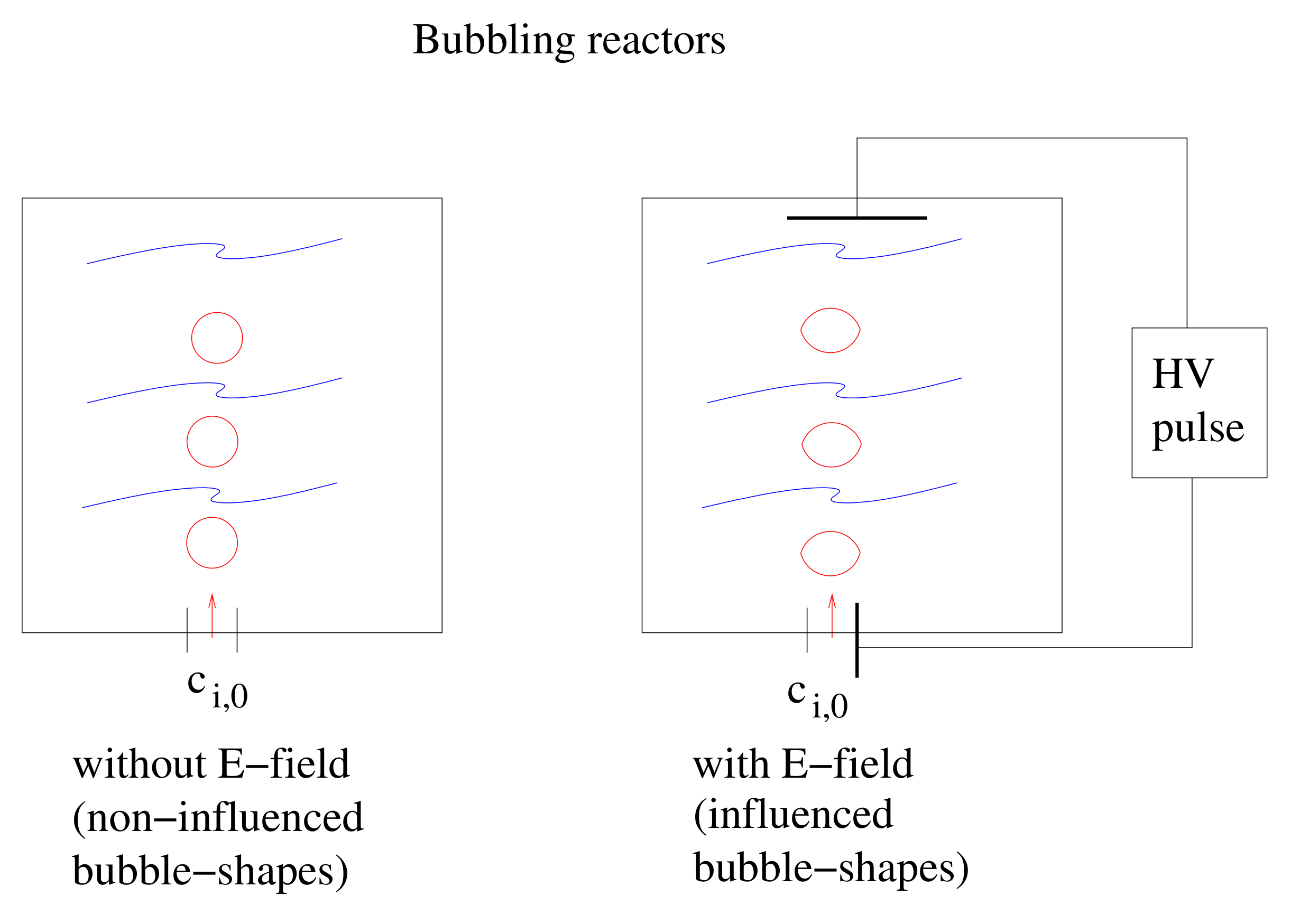
- The charged bubbles can be used as plasma bubbles and can be discharged, such applications can then be used to clean a polluted fluid, see [7].
- Fast ordinary differential equation (ODE) solvers for so-called bubble shape models, which are based on Young–Laplace equations: We apply the Young–Laplace equations, which are a system of ODEs. The benefit is that the solvers are very fast, while the drawback is that we are restricted to quasi-static processes, see [11].
- Coupled partial differential equation (PDE) solvers for so-called free surface models, which are based on Navier-Stokes equations with kinematic boundary condition. Here, we have to solve a free surface problem with PDE solvers. The benefit is that we can apply the model to instationary processes, the drawback is that we need to solve a system of PDEs, which is more time consuming, see [16].
- Volume-of-fluid (VOF) methods: the VOF function presents the fraction of the volume in the grid cells, which is occupied by one of the two fluids. This is modeled with an advection equation. The benefit of the methods are mass conservation, the drawback of the methods are the problem to solve the sharp change in interface-region, see [17,18].
- Level-set (LS) methods: the level set function presents a signed distance, which is positive on one fluid side and negative on the other fluid side, see [13]. It is also modeled with the same advection equation. The benefit of the methods is that we can solve if with fast high-speed flow methods, such as total variational diminishing (TVD) or essentially non-oscillatory (ENO) methods, see [19,20]. The drawback is the lack of mass conservation.
2. Mathematical Model
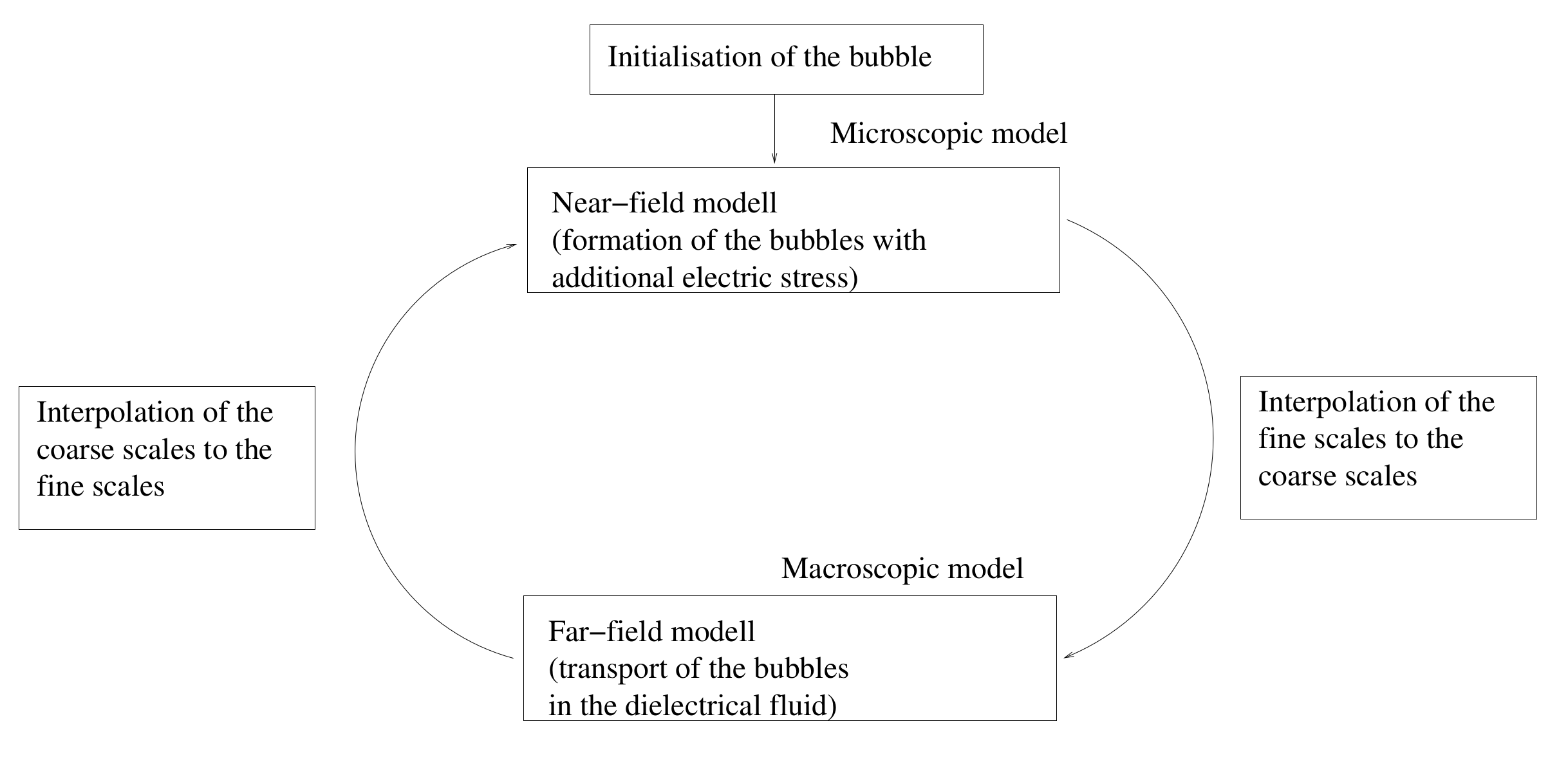
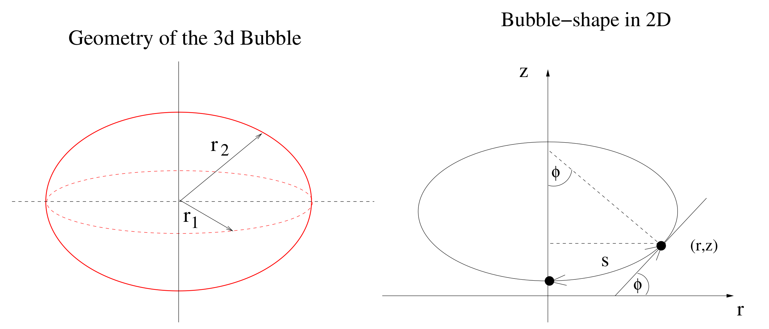
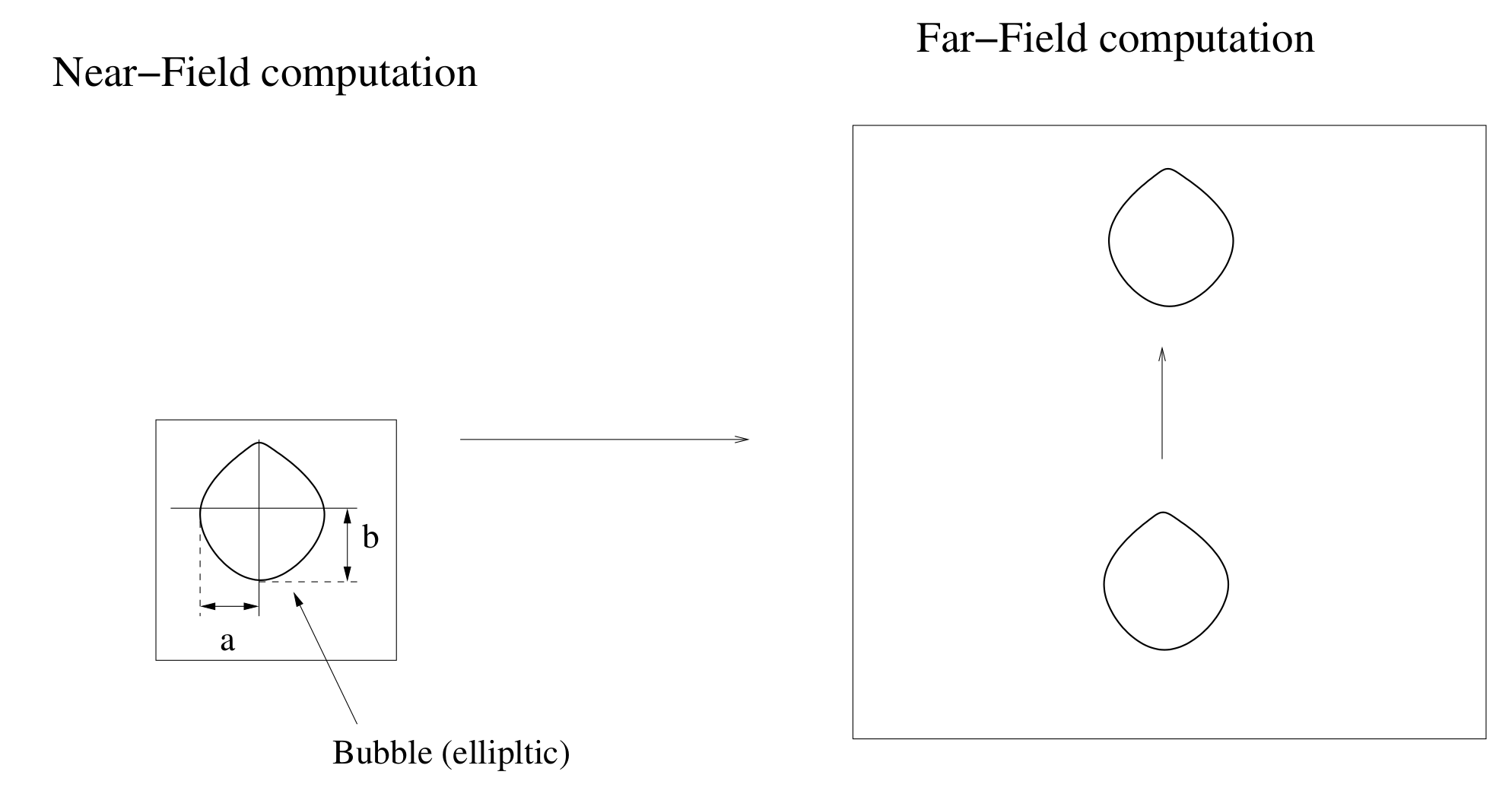
- Near-field approach, which is based on a Young–Laplace equation, see [11], where we have a static shape after the formation of the bubbles.
2.1. Electrical-Field Approach for the Near-Field Model
2.2. Near-Field Model
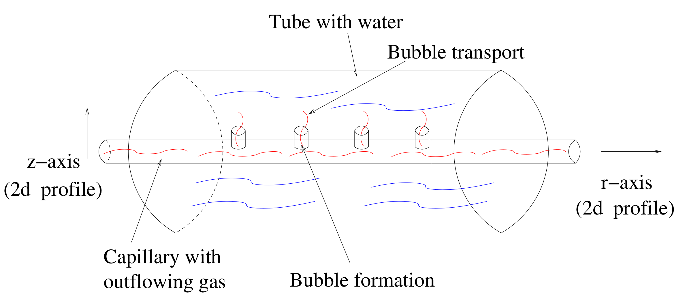
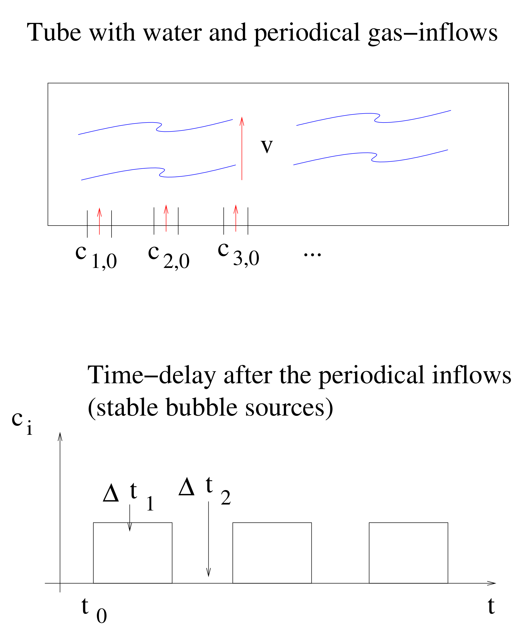
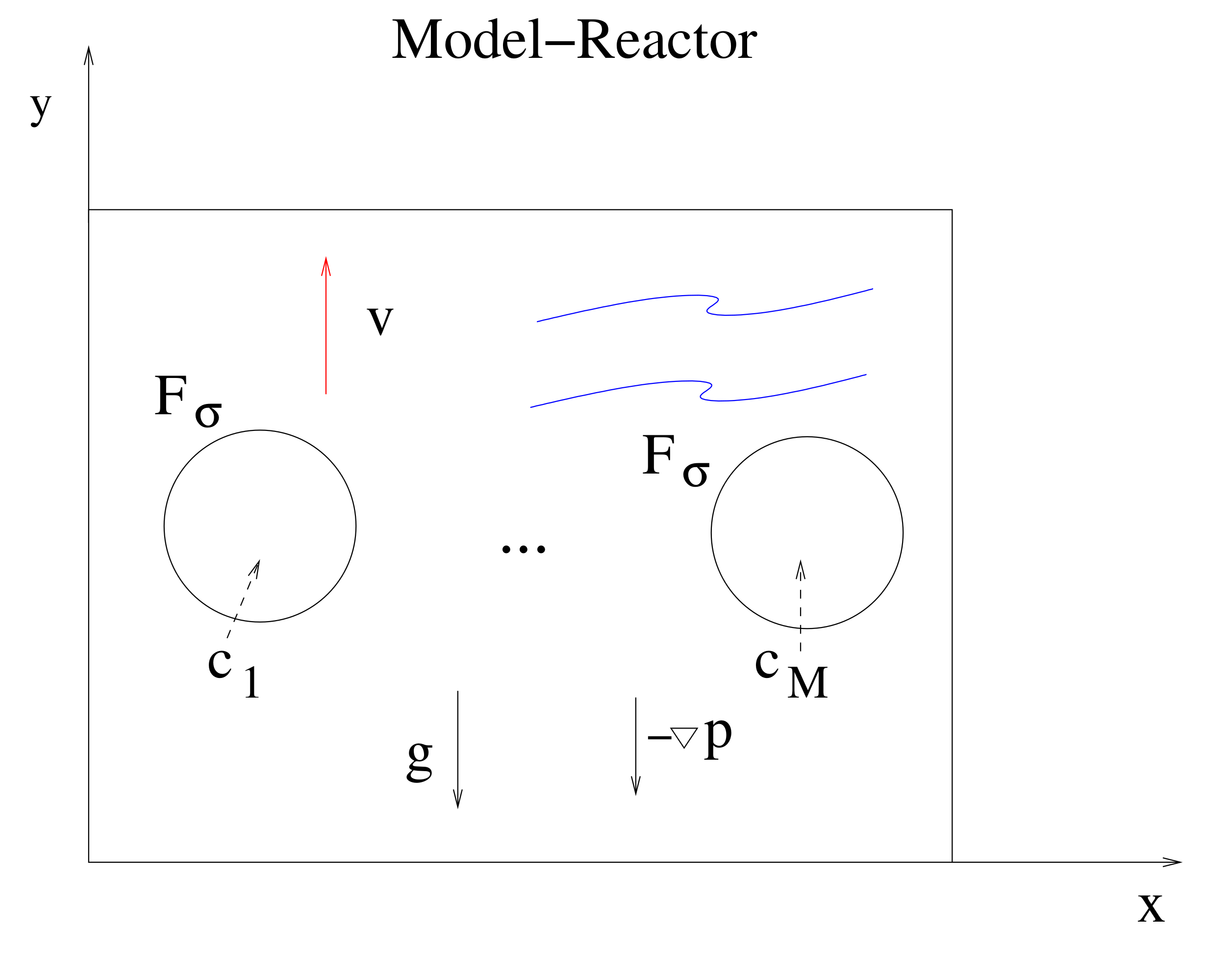
2.3. Far-Field Approach
- We can assume a constant velocity in the reactor.
- We assume that the water and the gas are not interacting or change the constant velocity.
- We have such small velocities, such that the transport equations of the gas bubbles are sufficient, see [18].
- The concentration of the bubbles are given as , while is the initial concentration of the bubble.
- Benefits:
- -
- The model is simple and fast to compute.
- -
- The model also allows us to discuss a dynamical shape.
- Drawbacks:
- -
- The shape of the bubble is not preserved, while we assume a static shape.
- -
- The influence of the speed of motion in the outer normal direction is not possible.
3. Near-Field Solver: System of Ordinary Differential Equations with Boundary Conditions
- For the grid-points , we denote by the solution of the initial value problem
- We approach to the grid and define a piecewiese function with
4. Far-Field Solver: Level-Set Method
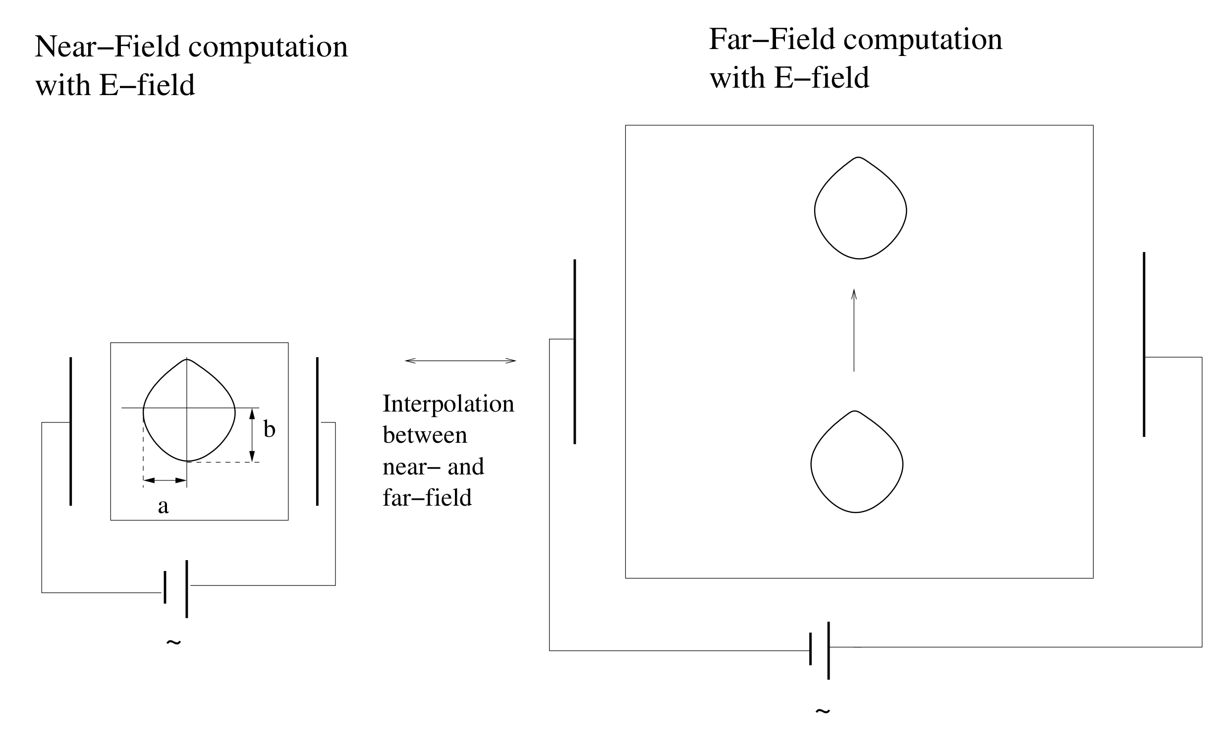
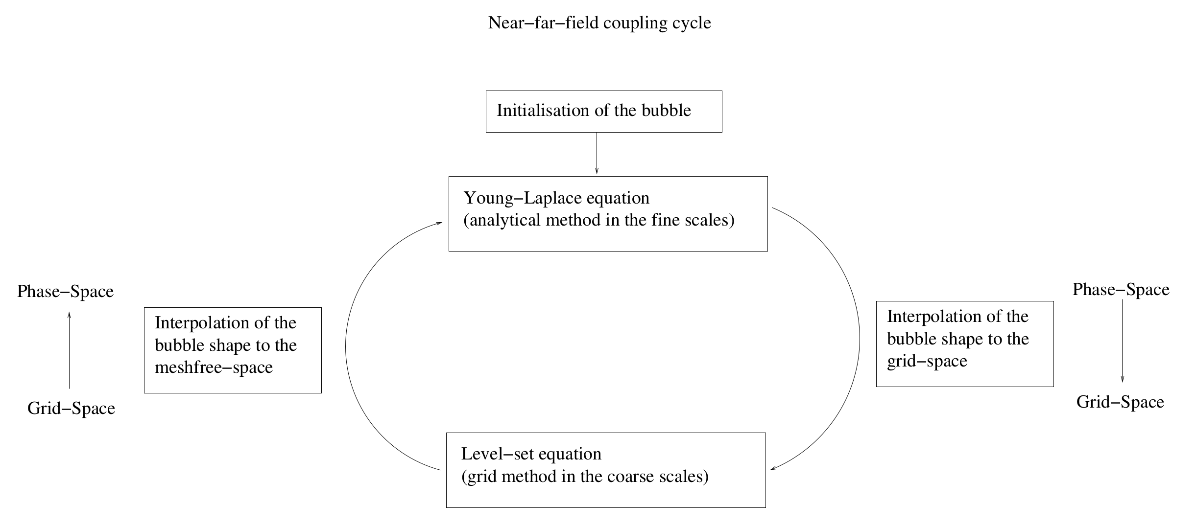
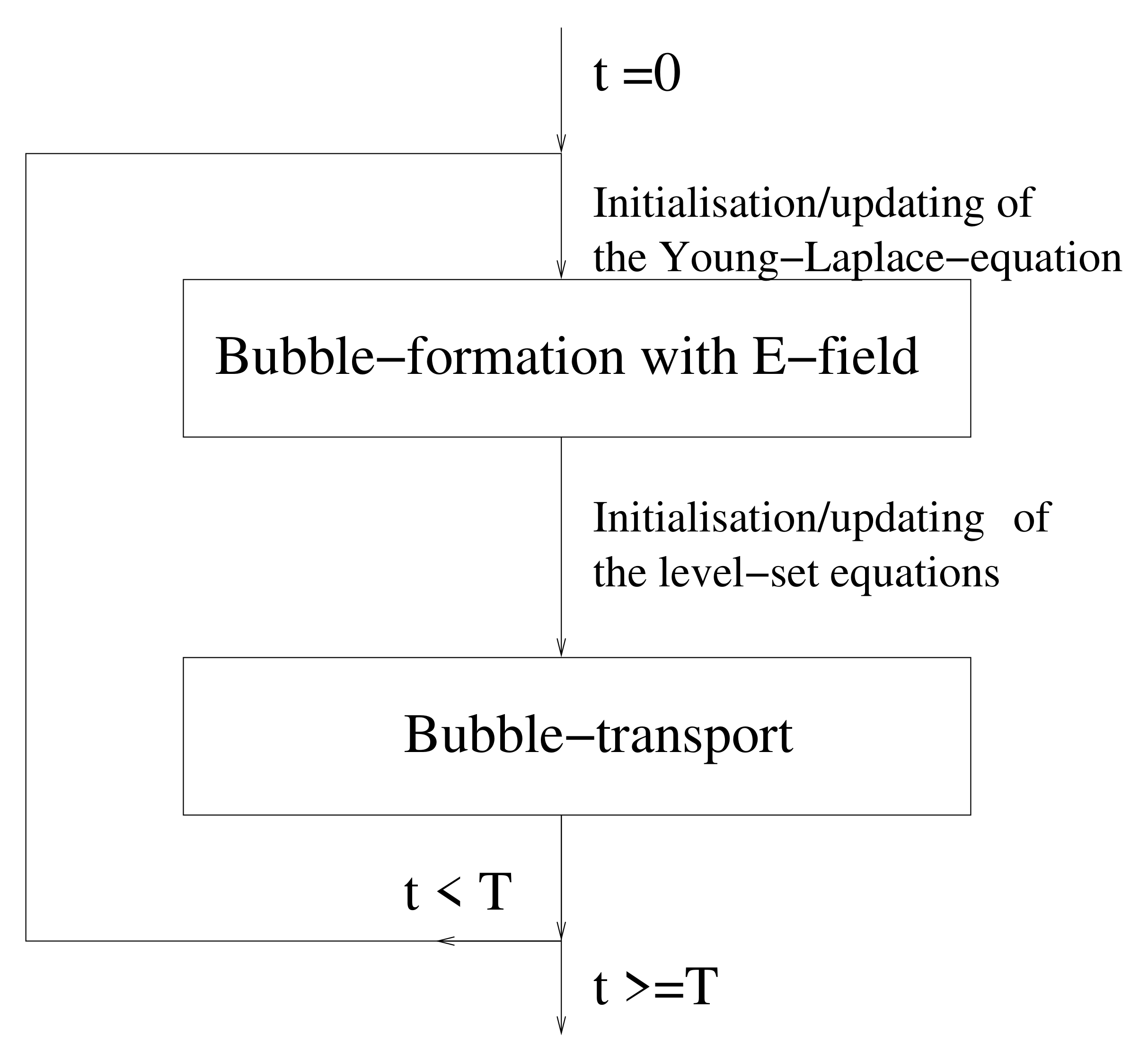
5. Coupling Near-Field and Far-Field
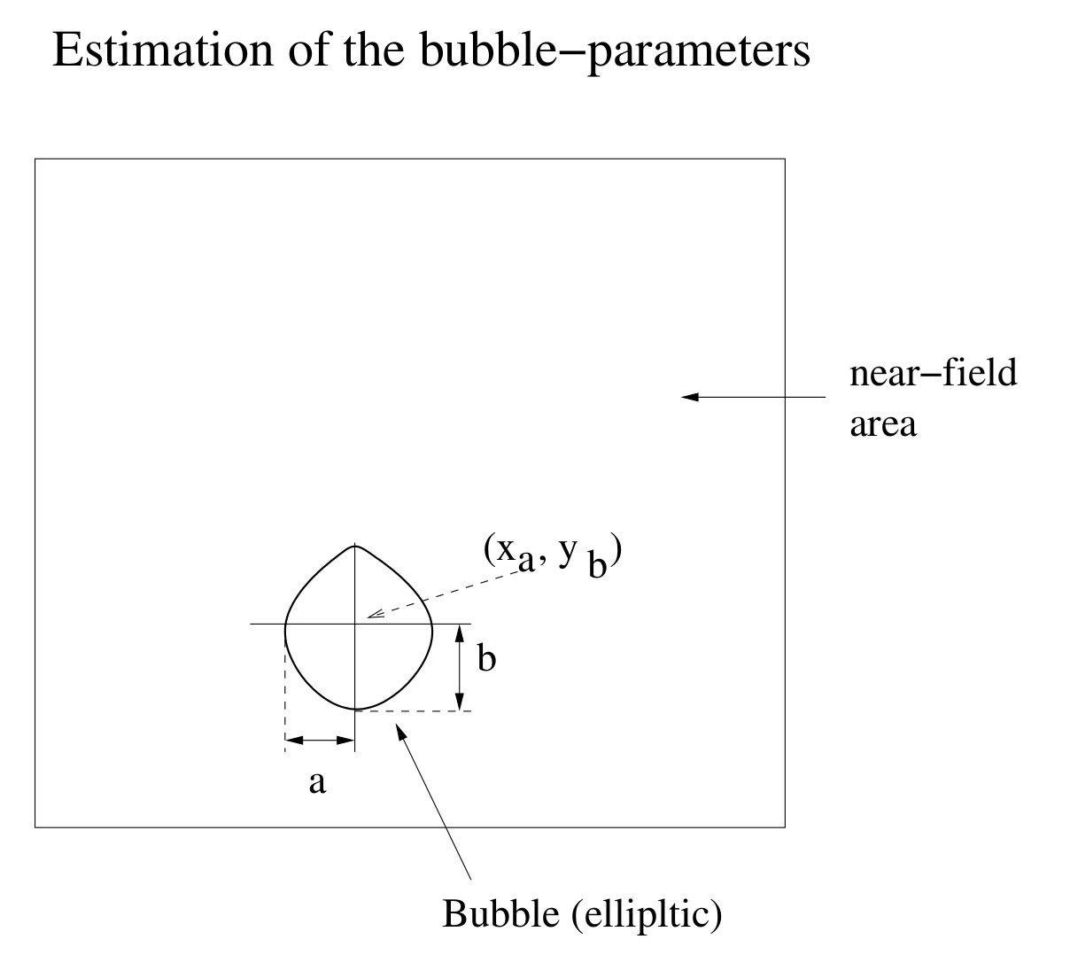
- Decoupled computation of near- and far-field: parameters of the ellipse are computed in the near-field and initialize the far-field bubble.
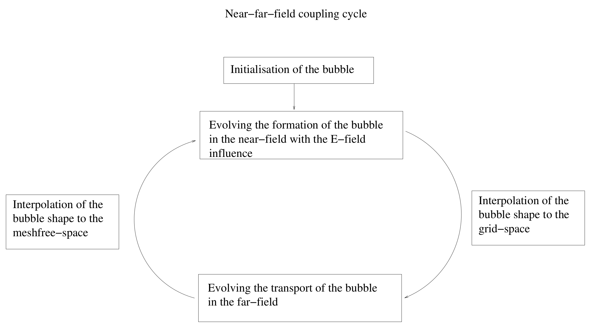
- Coupled computation of near- and far-field: the near-field computation is directly implemented into the far-field by a so-called bubble-in-cell (BIC) method and is directly updated in a computational cycle.
5.1. Decoupled Computation of Near- and Far-Field
5.2. Coupled Computation of Near- and Far-Field
6. Numerical Experiments
6.1. Bubble Formation: Experiment 1
- Test example 1:We apply the following test-example with the a quarter of a circle, means , where and we assume , where we assume is the arc-length step for the numerical computations. Further, we have .
- Test example 2:We have , where we assume is the arc-length step for the numerical computations. Further, we have and .
6.2. Bubble Formation: Validation of the Near-Field
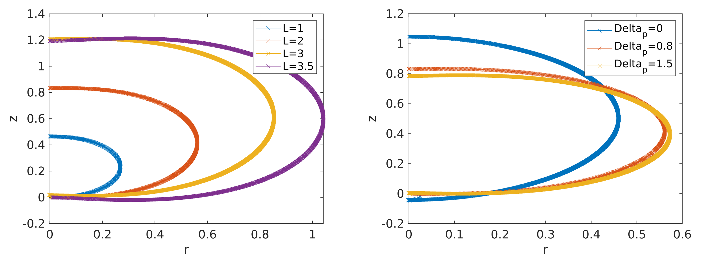
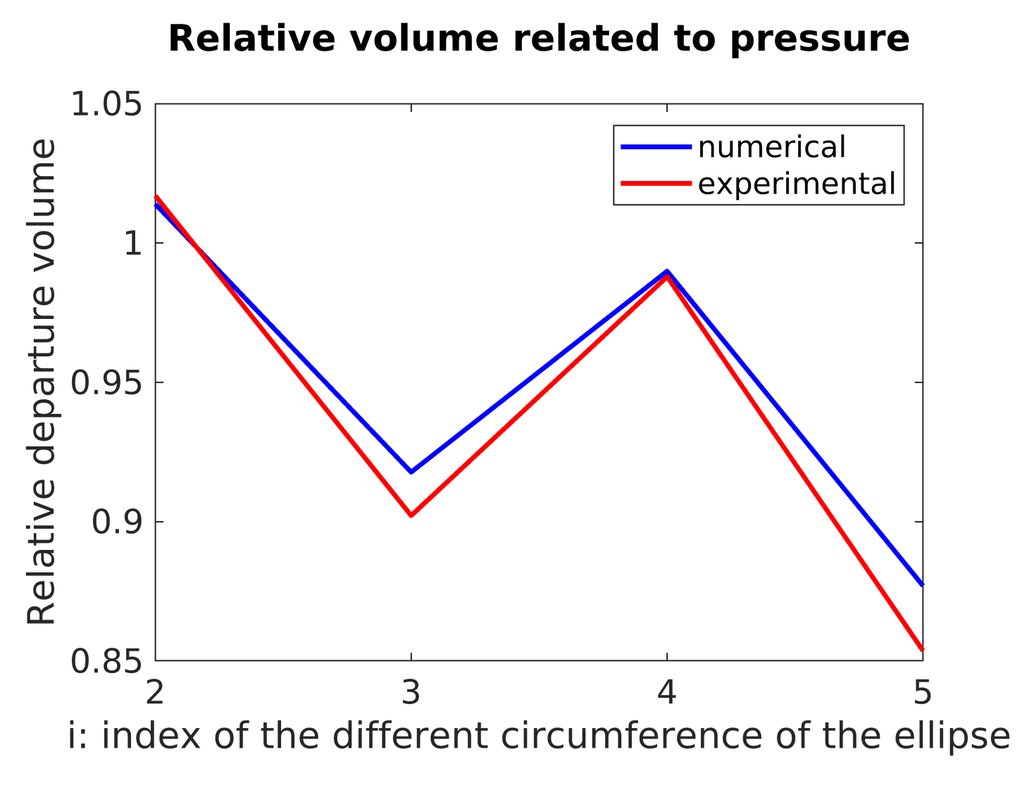
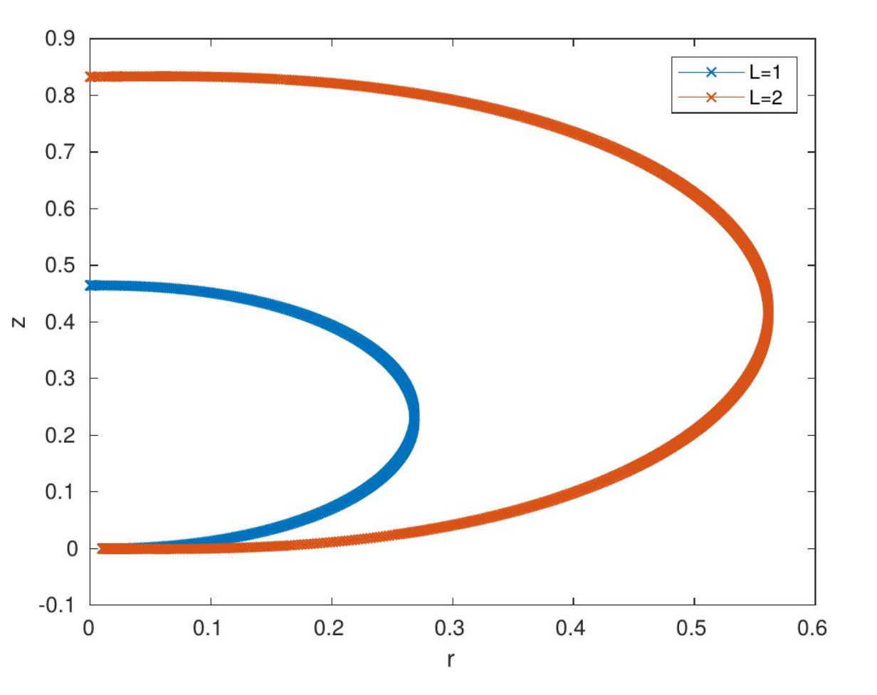
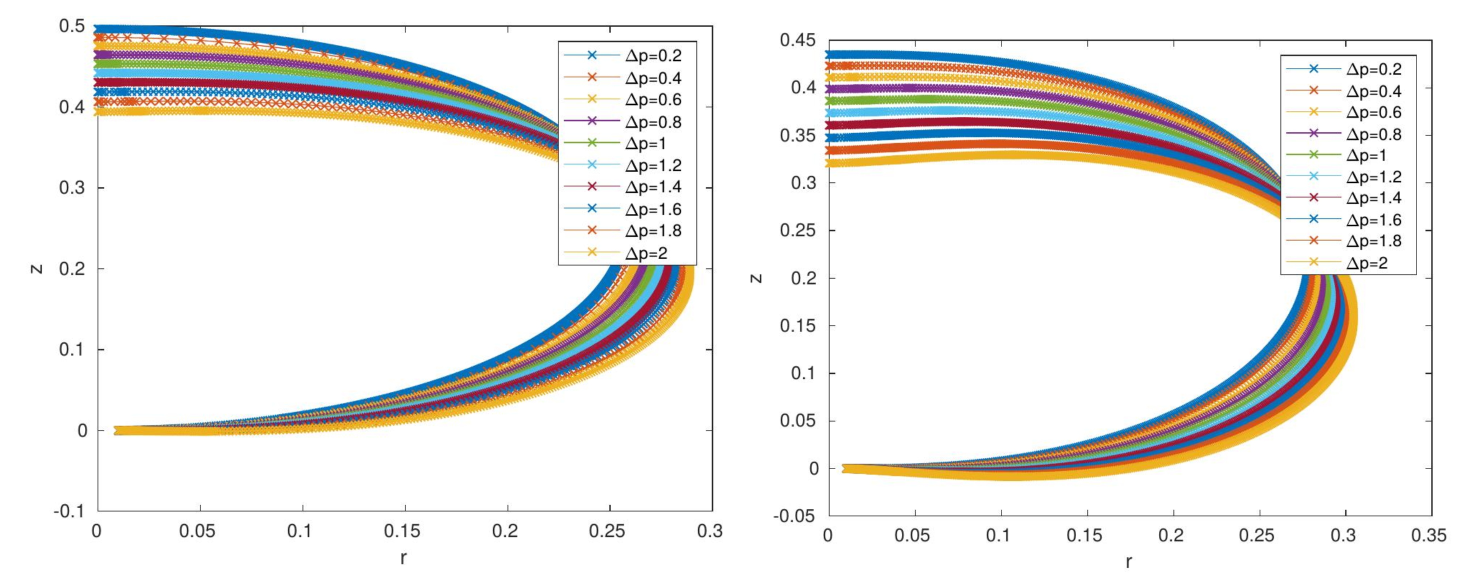
- Test example 1:We apply the following test-example with the circumference of the ellipse, which are given as , where , while a special case is the circle with and radius . Furthermore, we assume , where the arc-length step for the computations is and .Here, we measure prediction of the volume of the ellipsoid, while we assume a constant gas-flow-rate:means we apply:where , which we could compute with our MATLAB simulations. We assume that Q is a constant and approximated to V.Then, we can predict the departure volume with the experimental formula:where the constants are defined in Equation (58) and different volumes of the ellipsoids are given with the indices .
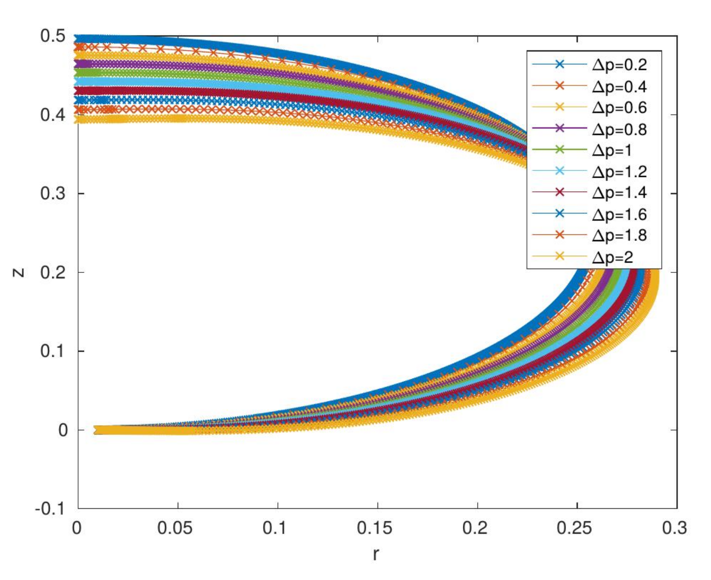
- Test example 2:We have , where the arc-length step for the computations is and and we apply the following pressure relations , , , and .Here, we can predict the different gas-flow-rates, based on the different pressure relations.where , which we could compute with our MATLAB simulations and we assume Q is a constant and approximated to V.
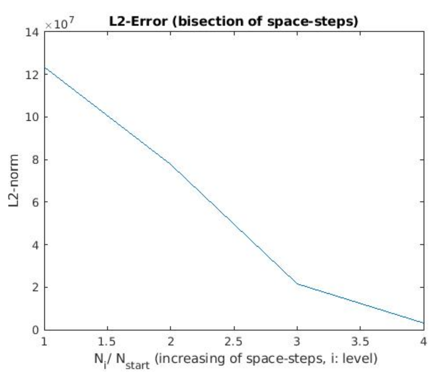
6.3. Bubble Transport: Validation of the Far-Field
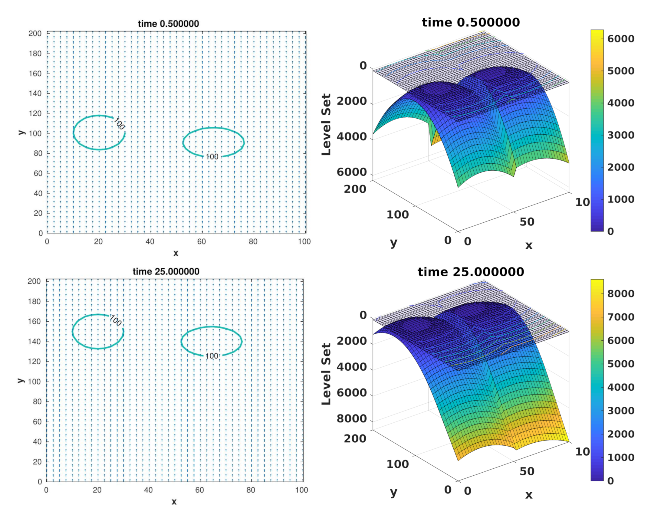
6.4. Bubble Formation: Experiment 2
- Input-parameters of the near-field bubbles:
- -
- ,
- -
- .
- We compute the bubbles based on the near-field code and we obtain the ellipse-diameters .
- We initialize the two ellipses for the far-field computations given as:
- ,
- .
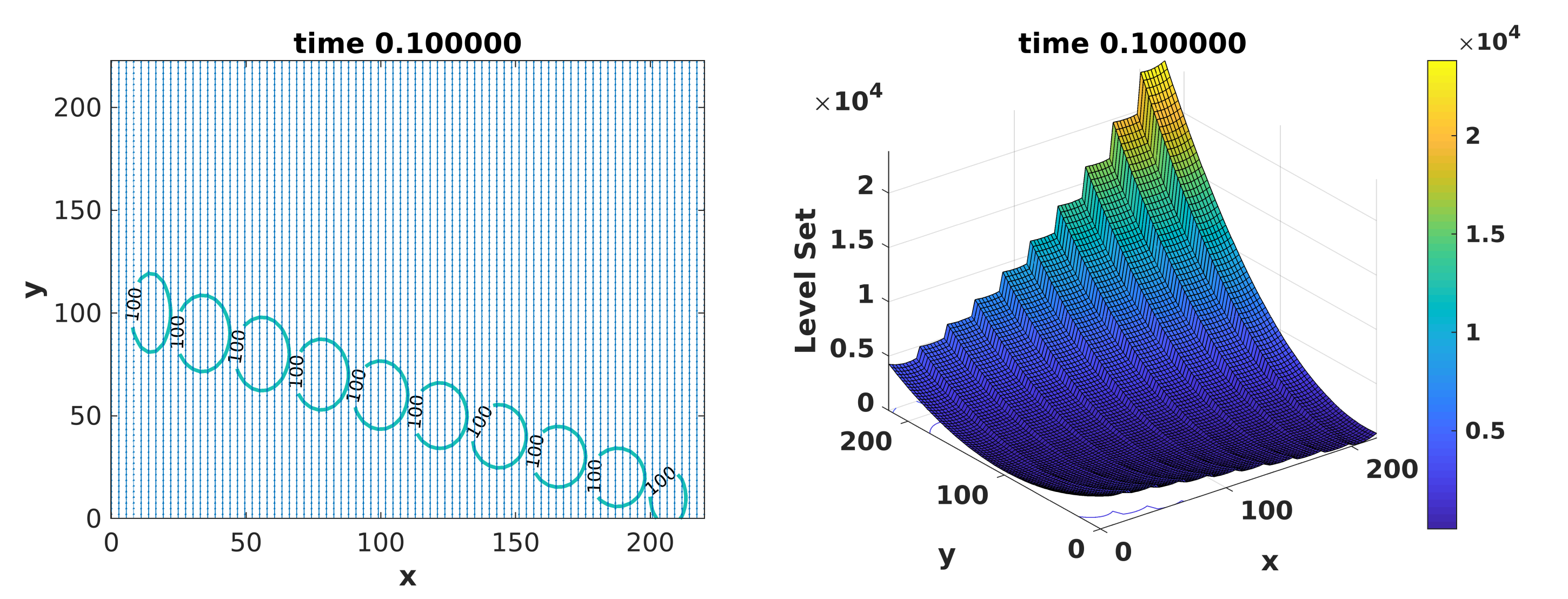
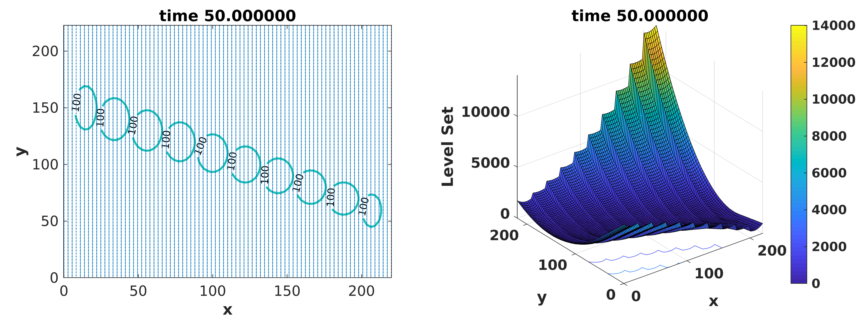
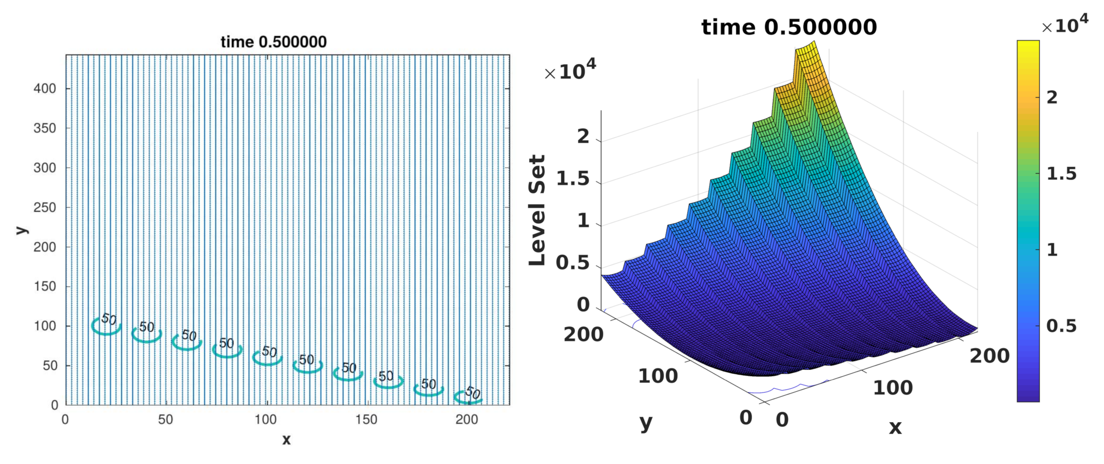
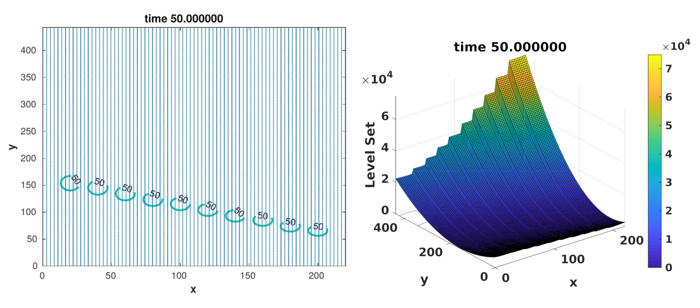
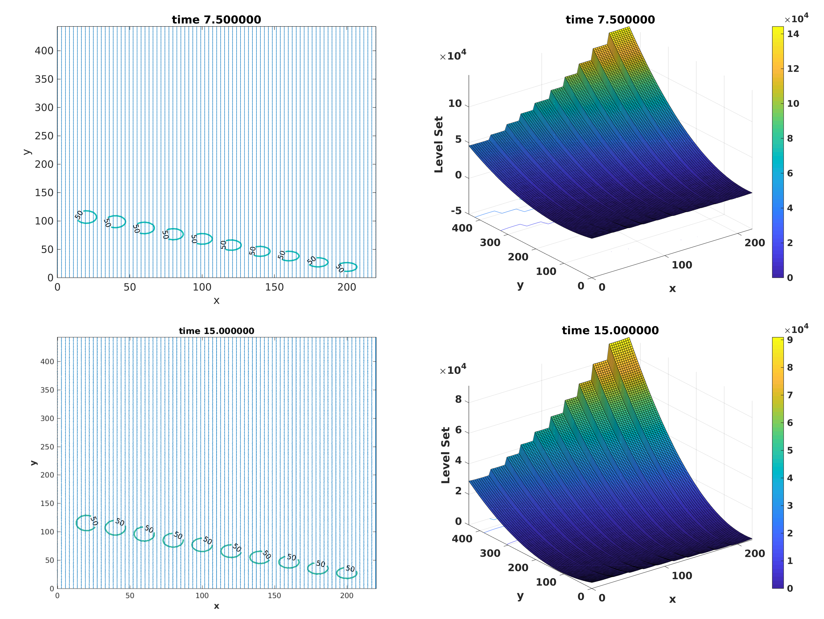
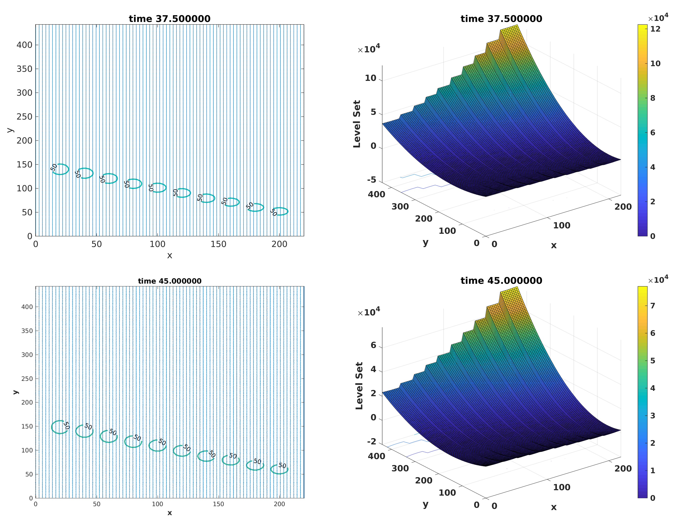
6.5. Bubble Formation: Multiple Bubble Experiment (10 Bubbles)
- Computation of the near-field bubbles (a representing bubble is computed):
- -
- Input-parameters of the near-field bubbles computation are given in Appendix A.1.
- -
- Output-parameters of the near-field bubble computation are given in Appendix A.1.
- -
- Ellipse: , where is the origin of the i-th bubble.
- Computation of the far-field bubbles (level-set initialization):
- -
- Parameterization of the level-set initial-function, such as two bubbles:where , with the coordinates of the grid and .
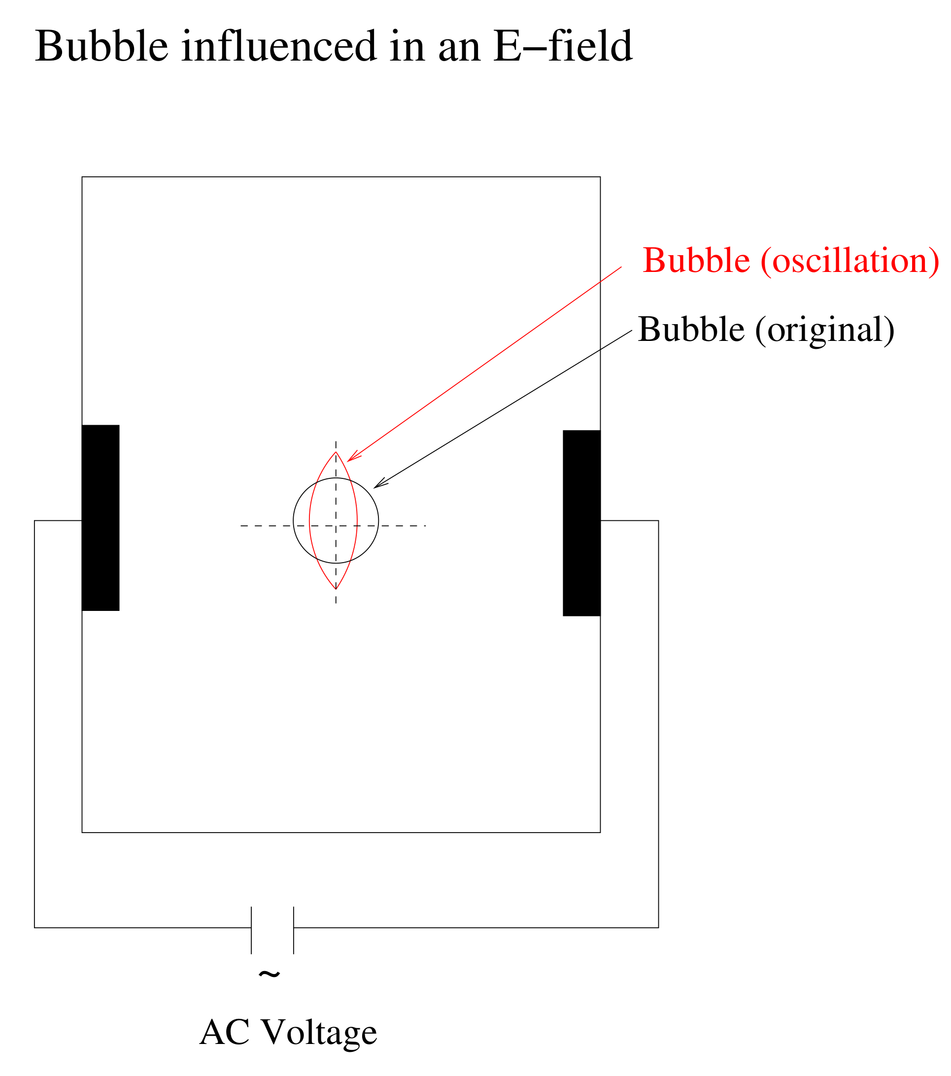
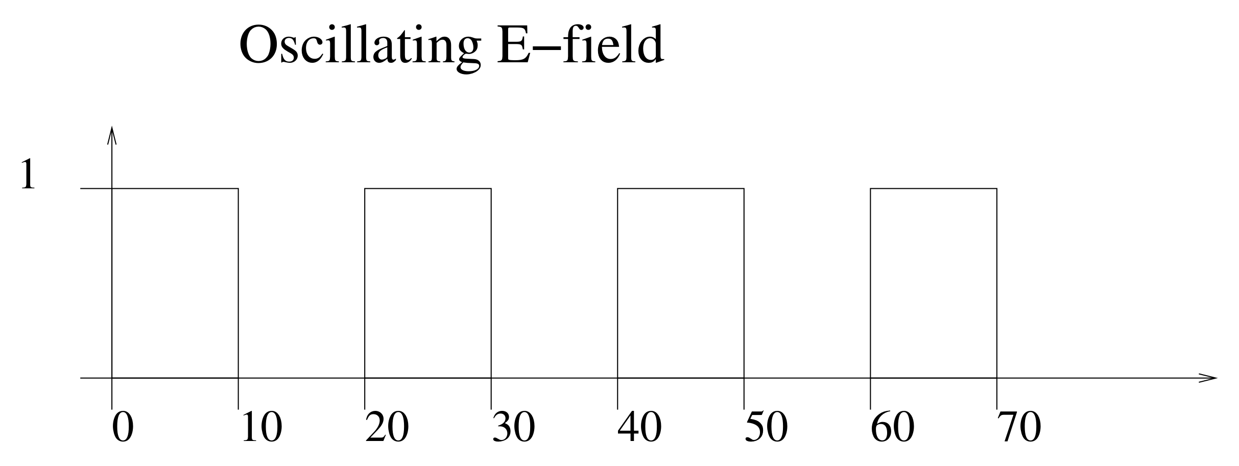
6.6. Bubble Formation: Oscillation of the Air-Bubbles in the Electrical-Field (Decoupled Version)
- Computation of the near-field bubbles (a representing bubble is computed)
- -
- The electrical field parameters are given as:, .
- -
- Input-parameters of the near-field bubbles computation are given in Appendix A.2.
- -
- Output-parameters of the near-field bubble computation (formation) are given in the Appendix A.2.
- -
- Output-parameters of the near-field bubble computation (in the E-field) are given in Appendix A.2.
- -
- Ellipse: , where is the origin of the i-th bubble.
- Computation of the far-field bubbles (level-set initialization):
- -
- Parameterization of the level-set initial-function, such as two bubbles:where , with the coordinates of the grid and .
6.7. Bubble Formation: Oscillation of the Air-Bubbles of an Oscillating Electrical- Field (Coupled Version)
7. Conclusions
Author Contributions
Funding
Acknowledgments
Conflicts of Interest
Appendix A.
Appendix A.1. Parameters of Section 6.5
- Input-parameters of the near-field bubbles computation:
- -
- Bubble 1: ,
- -
- Bubble 2: .
- -
- Bubble 3: .
- -
- Bubble 4: .
- -
- Bubble 5: .
- -
- Bubble 6: .
- -
- Bubble 7: .
- -
- Bubble 8: .
- -
- Bubble 9: .
- -
- Bubble 10: .
- Output-parameters of the near-field bubble computation:
- -
- Bubble 1: .
- -
- Bubble 2: .
- -
- Bubble 3: .
- -
- Bubble 4: .
- -
- Bubble 5: .
- -
- Bubble 6: .
- -
- Bubble 7: .
- -
- Bubble 8: .
- -
- Bubble 9: .
- -
- Bubble 10: .
Appendix A.2. Parameters of Section 6.6 and Section 6.7
- Input-parameters of the near-field bubbles computation:
- -
- Bubble 1: ,
- -
- Bubble 2: .
- -
- Bubble 3: .
- -
- Bubble 4: .
- -
- Bubble 5: .
- -
- Bubble 6: .
- -
- Bubble 7: .
- -
- Bubble 8: .
- -
- Bubble 9: .
- -
- Bubble 10: .
- Output-parameters of the near-field bubble computation (formation):
- -
- Bubble 1: .
- -
- Bubble 2: .
- -
- Bubble 3: .
- -
- Bubble 4: .
- -
- Bubble 5: .
- -
- Bubble 6: .
- -
- Bubble 7: .
- -
- Bubble 8: .
- -
- Bubble 9: .
- -
- Bubble 10: .
- Output-parameters of the near-field bubble computation (in the E-field):
- -
- Bubble 1: .
- -
- Bubble 2: .
- -
- Bubble 3: .
- -
- Bubble 4: .
- -
- Bubble 5: .
- -
- Bubble 6: .
- -
- Bubble 7: .
- -
- Bubble 8: .
- -
- Bubble 9: .
- -
- Bubble 10: .
References
- Gu, H.; Duits, M.H.G.; Mugele, F. Droplets formation and merging in two-phase flow microfluidics. Int. J. Mol. Sci. 2011, 12, 2572–2597. [Google Scholar] [CrossRef] [PubMed]
- Hayashi, T.; Uehara, S.; Takana, H.; Nishiyama, H. Gas-liquid two-phase chemical reaction model of reactive plasma inside a bubble for water treatment. In Proceeding of the 22nd International Symposium on Plasma Chemistry, Antwerp, Belgium, 5–10 July 2015. [Google Scholar]
- Kumar, R.; Kuloor, N.R. The formation of bubbles and drops. Adv. Chem. Eng. 1970, 8, 255–368. [Google Scholar]
- Yang, G.Q.; Du, B.; Fan, L.S. Bubble formation and dynamics in gas–liquid–solid fluidization—A review. Chem. Eng. Sci. 2007, 62, 2–27. [Google Scholar] [CrossRef]
- Ruzicka, M. Electrorheological Fluids: Modeling and Mathematical Theory; Lecture Notes in Mathematics; Springer: Berlin/Heidelberg, Germany, 2008; Volume 1748. [Google Scholar]
- Westerterp, K.R.; Swaaij, W.P.M.V.; Beenackers, A.A.C.M. Chemical Reactor Design and Operation, 2nd ed.; John Wiley and Sons: Chichester, UK; New York, NY, USA, 1984. [Google Scholar]
- Bruggeman, P.; Leys, C. Non-thermal plasmas in and in contact with liquids. J. Phys. D Appl. Phys. 2009, 42, 053001. [Google Scholar] [CrossRef]
- Besagni, G.; Inzoli, F.; Ziegenhein, T. Two-phase bubble columns: A comprehensive review. ChemEngineering 2018, 2, 13. [Google Scholar] [CrossRef]
- Mutabazi, I.; Yoshikawa, H.N.; Fogaing, M.T.; Travnikov, V.; Crumeyrolle, O.; Futterer, B.; Egber, C. Thermo-electro-hydrodynamic convection under microgravity: A review. Fluid Dyn. Res. 2016, 48, 061413. [Google Scholar] [CrossRef]
- Sommers, B.S.; Foster, J.E. Nonlinear oscillations of gas bubbles submerged in water: Implications for plasma breakdown. J. Phys. D Appl. Phys. 2012, 45, 415203. [Google Scholar] [CrossRef]
- Thoroddsen, S.T.; Takehara, K.; Etoh, T.G. The coalescence speed of a pendent and a sessile drop. J. Fluid Mech. 2005, 527, 85–114. [Google Scholar] [CrossRef]
- Geiser, J.; Arab, M. Porous Media Based Modeling of PE-CVD Apparatus: Electrical fields and Deposition Geometries. In Special Topics and Reviews in Porous Media; Begell House Inc.: Redding, CA, USA, 2010; Volume 1, pp. 215–229. [Google Scholar]
- Sethian, J.A. Level Set Methods: Evolving Interfaces in Geometry, Fluid Mechanics, Computer Vision, and Materials Science; Cambridge University Press: Cambridge, UK, 1996. [Google Scholar]
- Hockney, R.; Eastwood, J. Computer Simulation Using Particles; CRC Press: Boca Raton, FL, USA, 1985. [Google Scholar]
- Lapenta, G. DEMOCRITUS: An adaptive particle in cell (PIC) code for object-plasma interactions. J. Comput. Phys. 2011, 230, 4679–4695. [Google Scholar] [CrossRef]
- Simmons, J.A.; Shikhmurzaev, J.E.S.a.Y.D. The formation of a bubble from a submerged orifice. Eur. J. Mech. B Fluids 2015, 53 (Suppl. C), 24–36. [Google Scholar] [CrossRef] [Green Version]
- Hirt, C.W.; Nichols, B.D. Volume of fluid (VOF) method for the dynamics of free boundaries. J. Comput. Phys. 1981, 39, 201–225. [Google Scholar] [CrossRef]
- Tsui, Y.-Y.; Liu, C.-Y.; Lin, S.-W. Coupled level-set and volume-of-fluid method for two-phase flow calculations. Numer. Heat Transf. Part B Fundam. 2017, 71, 173–185. [Google Scholar] [CrossRef]
- Harten, A.; Chakravarthy, S.R. Multi-Dimensional ENO Schemes for General Geometries; USA, NASA Contractor Report 187637; ICASE Report No. 91–76; NASA Langeley Research Center: Hamption, VA, USA, 1991. Available online: https://ntrs.nasa.gov/search.jsp?R=19920001131 (accessed on 4 November 2019).
- Hu, C.; Shu, C.-W. Weighted essentially non-oscillatory schemes on triangular meshes. J. Comput. Phys. 1999, 150, 97–127. [Google Scholar] [CrossRef]
- Babaeva, N.Y.; Bhoj, A.N.; Kushner, M.J. Streamer dynamics in gases containing dust particles. Plasma Sources Sci. Technol. 2006, 15, 591–602. [Google Scholar] [CrossRef]
- Kushner, M.J. Modelling of microdischarge devices: Plasma and gas dynamics. J. Phys. D Appl. Phys. 2005, 38, 1633–1643. [Google Scholar] [CrossRef]
- Babaeva, N.Y.; Naidis, G.V.; Tereshonok, D.V.; Smirnov, B.M. Streamer breakdown in elongated, compressed and tilted bubbles immersed in water. J. Phys. D Appl. Phys. 2017, 50, 364001. [Google Scholar] [CrossRef]
- Brennen, C.E. Cavitation and Bubble Dynamics; Oxford University Press: New York, NY, USA; Oxford, UK, 1995. [Google Scholar]
- Geiser, J. Multicomponent and Multiscale Systems: Theory, Methods, and Applications in Engineering; Springer: Cham, Switzerland; Heidelberg, Germany; New York, NY, USA; Dordrecht, The Netherlands; London, UK, 2016. [Google Scholar]
- Osher, S.; Sethian, J.A. Fronts propagating with curvature-dependent speed: Algorithms based on Hamilton-Jacobi formulations. J. Comput. Phys. 1988, 79, 12–49. [Google Scholar] [CrossRef] [Green Version]
- Stratton, J.A. Electrodynamics Theory; Mc Graw Hill: New York, NY, USA, 1941; Chapter 3. [Google Scholar]
- Finn, R. Equilibrium Capillary Surfaces; Springer: New York, NY, USA, 1986. [Google Scholar]
- Vafaei, S.; Wen, D. Modification of the Young–Laplace equation and prediction of bubble interface in the presence of nanoparticles. Adv. Colloid Interface Sci. 2015, 225, 1–15. [Google Scholar] [CrossRef]
- Liu, L.; Russell, R.D. Linear system solver for boundary value ODEs. J. Comput. Appl. Math. 1993, 45, 103–117. [Google Scholar] [CrossRef]
- Osborne, M.R. On shooting methods for boundary value problems. J. Math. Anal. Appl. 1969, 27, 417–433. [Google Scholar] [CrossRef] [Green Version]
- Verführt, R. Numerical Methods and Stochastics, Part I: Numerical Methods; Lecture Notes Summerterm; Intitute of Mathematics, Ruhr-Unviersity of Bochum: Bochum, Germany, 2011. [Google Scholar]
- Bothe, D.; Koebe, M.; Wielage, K.; Prüss, J.; Warnecke, H.-J. Direct numerical simulation of mass transfer between rising gas bubbles and water. In Bubbly Flows: Analysis, Modelling and Calculation; Sommerfeld, M., Ed.; Springer: Berlin/Heidelberg, Germany, 2004; pp. 159–174. [Google Scholar]
- Leighton, T.G. The Acoustic Bubble; Academic Press: London, UK; San Diego, CA, USA, 1994. [Google Scholar]
- Weinan, E. Principle of Multiscale Modelling; Cambridge University Press: Cambridge, UK, 2010. [Google Scholar]
- Innocenti, M.E.; Lapenta, G.; Markidis, S.; Beck, A.; Vapirev, A. A multi level multi domain method for particle in cell plasma simulations. J. Comput. Phys. 2013, 238, 115–140. [Google Scholar] [CrossRef]
- Geiser, J.; Mertin, P. Modelling approach of a near-far-field model for bubble formation and transport. arXiv 2018, arXiv:1809.00899. [Google Scholar]
- Marmur, A.; Rubin, E. A theoretical model for bubble formation at an orifice submerged in an inviscid liquid. Chem. Eng. Sci. 1976, 31, 453–463. [Google Scholar] [CrossRef]
- Bellini, T.; Corti, M.; Gelmetti, A.; Lago, P. Interferometric study of selectively excited bubble capillary modes. Europhys. Lett. 1997, 38, 521–526. [Google Scholar] [CrossRef]
- Kröner, D. Numerical Schemes for Conservation Laws; Wiley-Teubner Series Advances in Numerical Mathematics; Wiley-Teubner: Chichester, UK, 1997. [Google Scholar]
- Geiser, J.; Buck, V.; Arab, M. Model of PE-CVD Apparatus: Verification and Simulations. Math. Prob. Eng. 2010, 2010, 407561. [Google Scholar] [CrossRef]


© 2019 by the authors. Licensee MDPI, Basel, Switzerland. This article is an open access article distributed under the terms and conditions of the Creative Commons Attribution (CC BY) license (http://creativecommons.org/licenses/by/4.0/).
Share and Cite
Geiser, J.; Mertin, P. A Near–Far-Field Model for Bubbles Influenced by External Electrical Fields. Appl. Sci. 2019, 9, 4722. https://doi.org/10.3390/app9214722
Geiser J, Mertin P. A Near–Far-Field Model for Bubbles Influenced by External Electrical Fields. Applied Sciences. 2019; 9(21):4722. https://doi.org/10.3390/app9214722
Chicago/Turabian StyleGeiser, Juergen, and Paul Mertin. 2019. "A Near–Far-Field Model for Bubbles Influenced by External Electrical Fields" Applied Sciences 9, no. 21: 4722. https://doi.org/10.3390/app9214722