Adaptive Network Based Fuzzy Inference System with Meta-Heuristic Optimizations for International Roughness Index Prediction

Abstract

The International Roughness Index (IRI) is the one of the most important roughness indexes to quantify road surface roughness. In this paper, we propose a new hybrid approach between adaptive network based fuzzy inference system (ANFIS) and various meta-heuristic optimizations such as the genetic algorithm (GA), particle swarm optimization (PSO), and the firefly algorithm (FA) to develop several hybrid models namely GA based ANGIS (GANFIS), PSO based ANFIS (PSOANFIS), FA based ANFIS (FAANFIS), respectively, for the prediction of the IRI. A benchmark model named artificial neural networks (ANN) was also used to compare with those hybrid models. To do this, a total of 2811 samples in the case study of the north of Vietnam (Northwest region, Northeast region, and the Red River Delta Area) within the scope of management of the DRM-I Department were used to validate the models in terms of various criteria like coefficient of determination (R) and the root mean square error (RMSE). Experimental results affirmed the potentiality and effectiveness of the proposed prediction models whereas the PSOANFIS (RMSE = 0.145 and R = 0.888) is better than the other models named GANFIS (RMSE = 0.155 and R = 0.872), FAANFIS (RMSE = 0.170 and R = 0.849), and ANN (RMSE = 0.186 and R = 0.804). The results of this study are helpful for accurate prediction of the IRI for evaluation of quality of road surface roughness.

1. Introduction

The International Roughness Index (IRI) is a standard index to quantify road surface roughness from measured longitudinal road profiles [1]. IRI is linearly proportional to roughness [2]; thus when the IRI value increases, the roughness of the pavement increases; and an IRI value of zero means that the pavement is smooth [3]. Some researchers reported that the pavement fails when IRI values reach 3 m/km, and an overlay is needed [3]. IRI is a standardized roughness measurement to represent the reaction of a single tire on a vehicle suspension to roughness in a pavement surface when a quarter car simulation traveling at 80 km/h [4]. In the literature, IRI can be determined from profiles obtained from high-speed inertial profiling systems [5]. Nonetheless, one problem associated with IRI is that determination of this index in laboratories is time-consuming and complicated, thus, the accurate prediction of the IRI is essential and useful.

Nowadays, machine learning (ML) methods have been applied widely in prediction of the IRI. Chen, et al. [6] proposed the grey forecast, genetic programming, and multiple regression for prediction the deterioration of IRI. Hossain, Gopisetti and Miah [3] used an artificial neural network (ANN) to predict the IRI for jointed plain concrete pavement sections. Lin, et al. [7] studied the relationships between IRI and pavement distress using a back-propagation neural network. Yousefzadeh, et al. [8] discussed road profile estimation using ANN. Mactutis, et al. [9] analyzed the relationship between the IRI and cracking and rutting over 317 observations. It has been inferred from these studies that good models and approaches should be developed in order to obtain higher prediction accuracy of IRI.

In this study, the main aim is to propose a new approach of adaptive network based fuzzy inference system (ANFIS) with various meta-heuristic optimizations namely the genetic algorithm (GA), particle swarm optimization (PSO), and the firefly algorithm (FA) to develop different hybrid models namely GA based ANGIS (GANFIS), PSO based ANFIS (PSOANFIS), FA based ANFIS (FAANFIS), respectively, for the prediction of the IRI. A benchmark model named ANN was also used to compare with those hybrid models. For this purpose, a total of 2811 samples in the case study of the north of Vietnam (Northwest region, Northeast region, Red River Delta Area) within the scope of management of the DRM-I Department were used to validate the proposed and applied models in terms of various criteria like coefficient of determination (R) and root mean square error (RMSE).

2. Materials and Methods

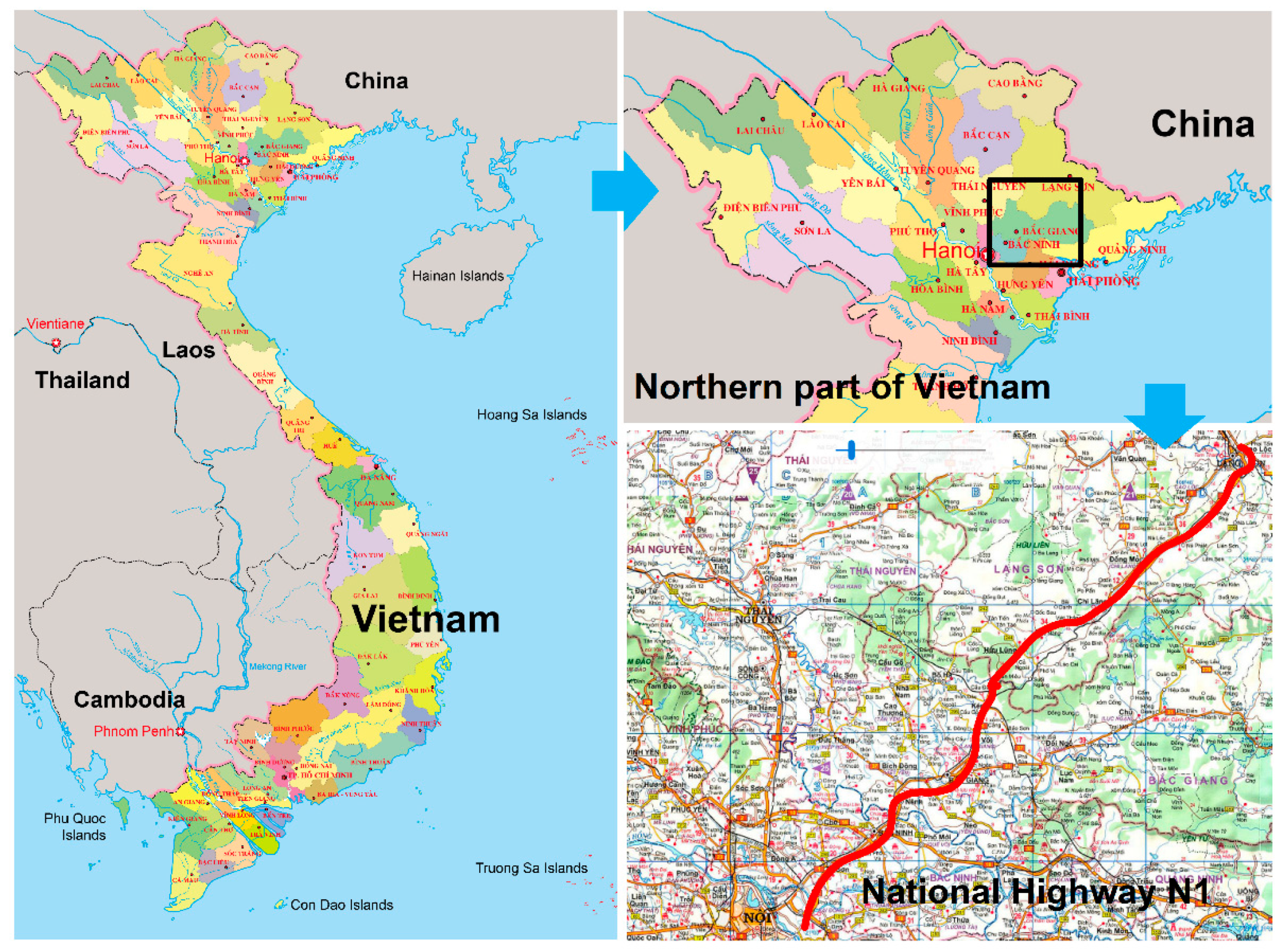
2.1. Case Study and Database

In this study, the data of the road surface status were collected by the Vietnam Road Administration in coordination with the Japanese International Cooperation Agency (JICA) from April 2012 to March 2013 for each 100 m of lane for the entire national road network. This area is located in the north of Vietnam (Northwest region, Northeast region, Red River Delta Area) (Figure 1). The survey was conducted for two types of pavements including cement and asphalt concrete pavements. For the asphalt concrete pavement, it was implemented for the expressway and national highway (including newly operated and operated highways) named National Highway N1 (Figure 1). The content of survey consisted of scale, survey period, diagram of lane layout and survey direction, and survey parameters. The survey parameters contained a type of car survey, vehicle weight, air pressure of wheel, the surface temperature, testing apparatus, and testing method. This project was particularly important because of the need for surveying and collecting road surface status data, especially for expressways that ensure comprehensiveness, accuracy, speed, efficiency, economics, and the ability to not obstruct current traffic in Vietnam. Therefore, Hawkeye technology was a good method for road management, maintenance and operation units to meet new requirements on surveying and managing data at all levels (https://arrbsystems.com/hawkeye-1000-series/). Since then, there have been effective plans and solutions in road maintenance and operation.

Data include three basic characteristics of the road surface namely the international roughness of IRI, the depth of the track and the depth of road surface cracking. In addition, the GPS coordinates of points on the road and the image of the road were automatically recorded continuously according to the recording step of 5 m. A total of 2811 samples were collected and tested to generate the datasets which includes road length (m), analysis area (${\mathrm{m}}^2$), summed cracks, maximum depth of ruts (mm), average depth of ruts (mm), and IRI (mm/m) (

Table 1. Data presentation.

X1	X2	X3	X4	X5	Y
90	340.2	0	31	9	10.25
100	344	0	13	6	5.5
100	327	0	10	6	2.93
100	324	2.9	15	7	2.95
100	328	0	11	8	2.3
…	…	…	…	…	…
…	…	…	…	…	…
…	…	…	…	…	…
25	91.5	0	9	6	4.3
100	360	0	12	7	4.36
100	349	0	17	9	5.78
100	336	2	21	9	9.08
100	344	0	25	12	7.39

).

Table 2. Statistical Measures of Dataset Features.

Criteria	X1	X2	X3	X4	X5	Y
Mean	89.893	306.860	2.376	23.077	11.618	3.072
Std	26.776	92.131	7.937	13.685	3.289	1.904
Min	5	15.2	0	5	3	0.720
25%	100	328	0	16	9	2.190
50%	100	338	0	19	11	2.600
75%	100	346	0	24	14	3.265
Max	100	380	100	119	33	37.520

describes the statistical measures of dataset features.

In modeling, IRI was taken into account as the output variable (Y) while other parameters, which were road length, analysis area, summed cracks, maximum depth of rut, average depth of rut, were considered to be the independent variables X₁, X₂, X₃, X₄, X₅, respectively. There were two parts generated from the original data. The first part data was a training dataset, which stood at 70% as opposite to that of the validating dataset (30%). The validating dataset was then used to test the models while training dataset was used to learn them. In the meantime, the principal component analysis method (PCA) [10] was used to reduce the dimensions data. Thus, we only selected the features which carry important information, and eliminated the irrelevant features for prediction. Savitzky–Golay filtering [11] was also applied in order to reduce extreme values in the distribution of data. This noise reduction technique was necessary in order to track nonlinear relationship between inputs and outputs without changing its tendency. In this paper, third degree polynomial and a window size of 15 were used when applying the Savitzky–Golay filtering technique. Finally, in order to deal with real values of measurement on different scales, all data were normalized into the [−1,1] range.

2.2. Methods Used

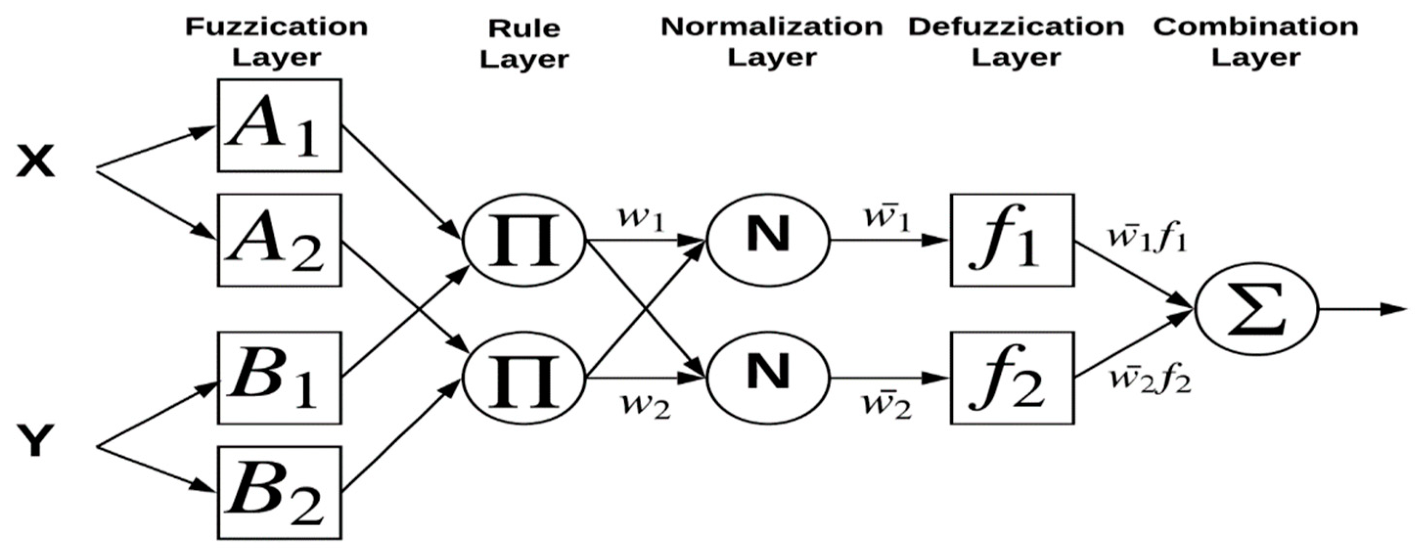
2.2.1. Adaptive Neural Fuzzy Inference System (ANFIS)

ANFIS is a powerful Artificial Intelligent prediction system that uses combination of ML technique of neural networks and a fuzzy logic system [12,13,14]. The ANFIS structure was a five-layer as follows [15] (Figure 2):

Layer 1: This was the fuzzification layer. It consisted of defined membership functions of the input variables. The output was a degree of membership value that was calculated based on a Gaussian membership function.

$${\mu }_{Ai}\left(x\right)=\exp \left[-{\left(\frac{x-c_i}{2{\delta }_i^2}\right)}^2\right]$$

(1)

where $c_i$, ${\delta }_i$ are parameters of a membership function.

Layer 2: This layer executed fuzzy AND of the previous part of the fuzzy rules.

$$w_i={\mu }_{Ai}\left(x\right)\ast {\mu }_{Bi}\left(x\right)$$

(2)

Layer 3: This was the normalized layer. This layer normalized the membership functions.

$${\overline{w}}_i=\frac{w_i}{{{\displaystyle \sum }}_i{w}_i}$$

(3)

Layer 4: This was the defuzzification layer. This layer executed the consequent part of the fuzzy rules.

$${\overline{w}}_i{f}_i={\overline{w}}_i\left(p_{i}x+q_{i}y+r_i\right)$$

(4)

where $p_i$, $q_i$, $r_i$ are linear parameters.

Layer 5: This output and combination layer was calculated by summing up the outputs of previous layers.

$${\displaystyle \sum }_i{\overline{w}}_i{f}_i=\frac{{{\displaystyle \sum }}_i{w}_i{f}_i}{{{\displaystyle \sum }}_i{w}_i}$$

(5)

2.2.2. Particle Swarm Optimization (PSO)

PSO is inspired by the behavior of biological communities like a swarm of insects so as to look for best solution in a given space [16]. The original PSO algorithm was initially proposed by Kennedy and Eberhart in [17]. It generally includes a population of candidate and the particles which are solutions. PSO is initiated by a random cluster of individuals, then search for the optimal solution by updating the generation [18]. In each generation, two values such as Pbest and Gbest are used to update each individual [19]. The process of updating individuals was based on the following two formulas:

$$x_i^{k+1}=x_i^k+v_i^{k+1}$$

(6)

$$v_i^{k+1}=v_i^k+c_1{r}_1\left(p_i^k-x_i^k\right)+c_2{r}_2\left(p_g^k-x_i^k\right)$$

(7)

where $x_i^k$: particle position, $v_i^k$: particle velocity, $p_i^k$: the best location of individual $i$ in the swarm, $p_g^k$: the best location of the all individual in the swarm, $c_1,c_2$: cognitive and social parameters, $r_1, r_2$: random number, range from 0 to 1.

2.2.3. Genetic Algorithm (GA)

GA is based on Darwin’s theory of evolution [20]. GA uses the principles of genetics, mutation, natural selection and cross-exchange. It includes a number of genome terms such as chromosomes, populations, and genes. Chromosomes are made up of genes. Each gene carries several characteristics and is located in the chromosome. Each chromosome will represent a solution to the problem [21].

The algorithm was carried out in the following steps [22]:

Step 1:

Population Initiation: Generated randomly a population of n individuals (where n is the solution to the problem).

Step 2:

Estimated the adaptation value of each individual.

Step 3:

Stop Condition: Checked the condition to terminate the algorithm.

Step 4:

Selection: Selected two parents from the old population according to their adaptation.

Step 5:

Cross exchange: With a selected probability, there was a new one which was created by the crossing exchange of two parents.

Step 6:

Mutation: With a selected mutation probability, the new individual was mutated.

Step 7:

Select the result: If the stop condition was satisfied, the algorithm terminated and chose the best solution in the current population.

GA had two basic stop conditions:

Condition 1.

Based on the chromosome structure, controlling the number of genes that were converging. If the number of genes converged at or beyond that point, the algorithm terminated.

Condition 2.

Based on the special meaning of the chromosome, it measured the change of the algorithm after each generation. If this change was less than a fixed constant, the algorithm terminated.

2.2.4. Firefly Algorithm (FA)

FA solves the hardest optimization problems based on the flashing patterns and behavior of fireflies. The original FA algorithm was initially developed by Yang [23]. Generally, FA used the three rules as follows:

(1)

The fireflies were unisex so that a firefly was attracted to all other fireflies regardless of their sex.

(2)

Attractiveness of a firefly was proportional to its brightness. The firefly moved randomly as there was no brighter firefly nearby.

(3)

Brightness of a firefly was determined by the value of its objective function.

Movement of a firefly was based on the following two formulas:

$$x_i^{k+1}=x_i^k+{\beta }_0{e}^{-\gamma r_{ij}^2}\left(x_j^k-x_i^k\right)+\alpha (rand()-0.5)$$

(8)

$$\beta ={\beta }_0{e}^{-\gamma r^2}$$

(9)

where $\beta$ is defined as the attractiveness degree of a firefly at an r distance, ${\beta }_0$ is the attractiveness degree of a firefly at a distance r = 0, $\gamma$ is the light absorption coefficient, and Rand () is a random number, which refers to the uniform distribution on (0, 1).

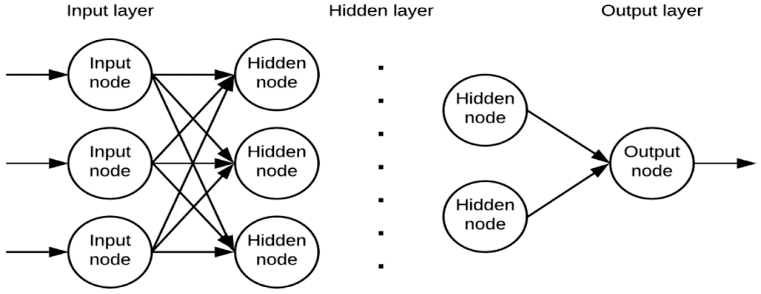
2.2.5. Artificial Neural Network (ANN)

ANN is inspired by the way of biological nervous system like human brain processes information [24]. A basic ANN contains artificial neurons including three simple sets of rules: multiplication, summation and activation. At the entry, the input are multiplied by its corresponding weight [24]. Neural networks use weights information which express the strength of the interconnection to address the problem. Then, all weighted inputs are all summed up inside computing unit [24]. The last section of the artificial neuron is transfer function, in which the sum is passed through activation function such as sigmoid, tanh, and rectified linear unit (RLU) [24,25].

When combining two or multiple basic artificial neurons (nodes), we are getting an artificial neural network. In a typical ANN, there are different layers: input layers, hidden layers and output layers [26] (Figure 3). Nodes at each layer have different functions. Input nodes are simply weighted and summed. Hidden nodes have no direct connection to the incoming data or to the ultimate output. They receive input from previous hidden nodes or initial input, then producing output to next hidden nodes or ultimate output. Output nodes assume responsibility for computations and transferring information to the outside.

2.2.6. Accuracy Validation

Accuracy of the proposed and applied models was validated by the coefficient of determination (R) and the root mean square error (RMSE) [27,28,29,30]. RMSE is the average squared difference between outputs and targets [31]. It is always positive and its units match the units of the response. Lower RMSE values are better [32,33]. The R values measure the correlation between outputs and targets [34,35,36,37]. While R can be more easily interpreted, RMSE can be know the amount of predictions deviate, on average, from the actual values in the dataset [31]. The formulas were as follow [38,39,40,41]:

$$RMSE=\sqrt{{\displaystyle \sum }_{i=1}^n\frac{{\left(p{r}_i-y_i\right)}^2}{n}}$$

(10)

$$R=\frac{{{\displaystyle \sum }}_{i=1}^n\left(p{r}_i-\overline{pr}\right)\left(y_i-\overline{y}\right)}{\sqrt{{{\displaystyle \sum }}_{i=1}^n{\left(p{r}_i-\overline{pr}\right)}^2}\sqrt{{{\displaystyle \sum }}_{i=1}^n\left(y_i-\overline{y}\right)}}$$

(11)

where $p{r}_i$ and $\overline{pr}$ are inferred as output values from the models, $y_i$ and $\overline{y}$ are the actual and mean values of IRI, respectively, and n is defined as the number of input data.

In addition to above validation criteria, a non-parametric test named Wilcoxon sign-ranked test was used in this study to evaluate that whether the difference of the accuracy among the models are statically significant [42]. This test was based on a predominant null hypothesis that there was no difference between the models at the significant level of α = 0.05, and that statistical values such as the z-value and p-value were calculated [42]. If z-value and p-value were out of the range from −1.96 and +1.96 and smaller than 0.05, respectively, the null hypothesis was rejected, which means the difference between the models was statically significant and vice versa [43].

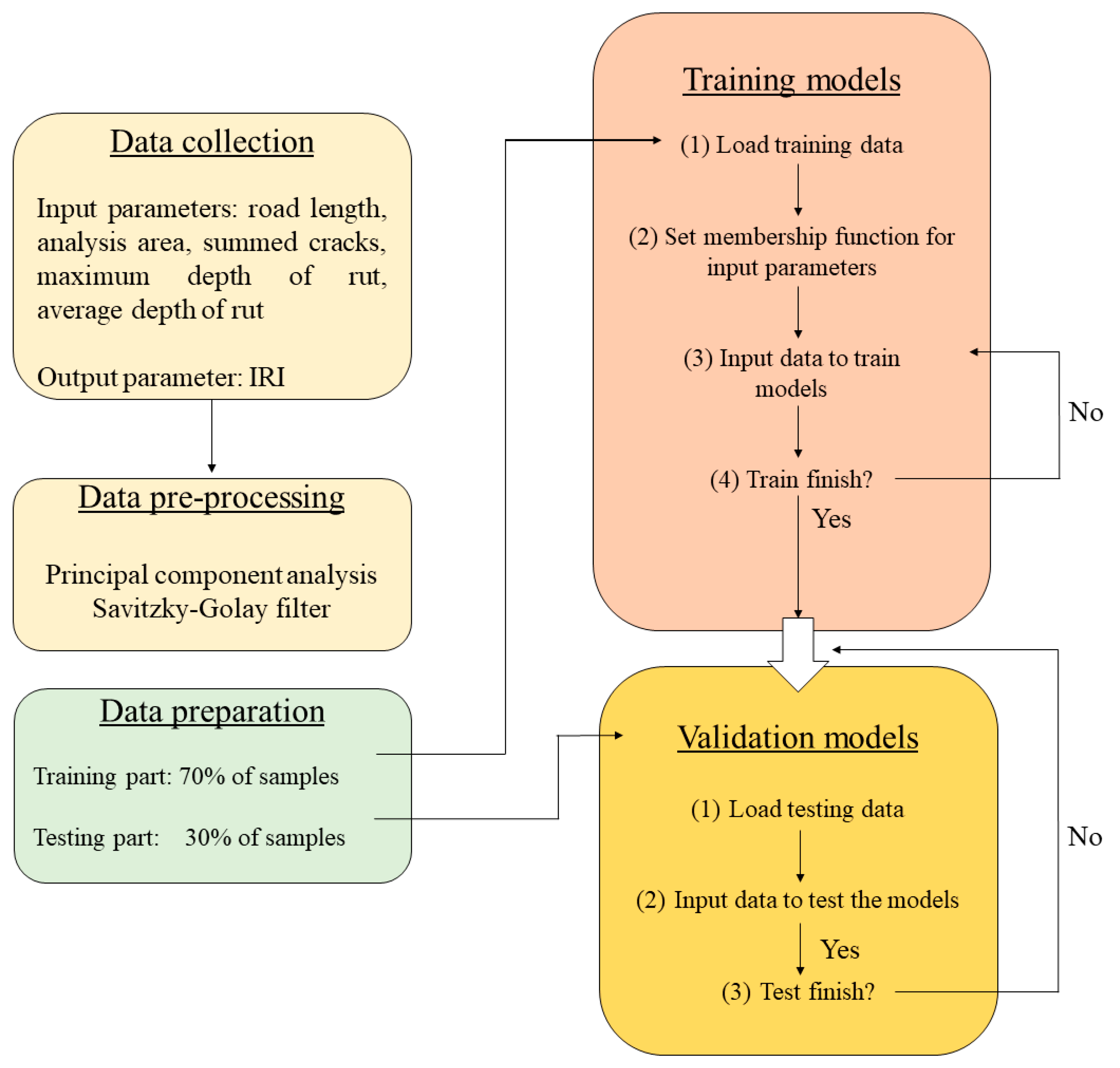
2.3. Methodology Framework

The modeling procedure for the prediction of IRI was carried out in four main steps: (I) data collection, (II) data preparation, (III) training models, and (IV) validation of models. A detailed description of each is briefly recalled below (Figure 4):

(i)

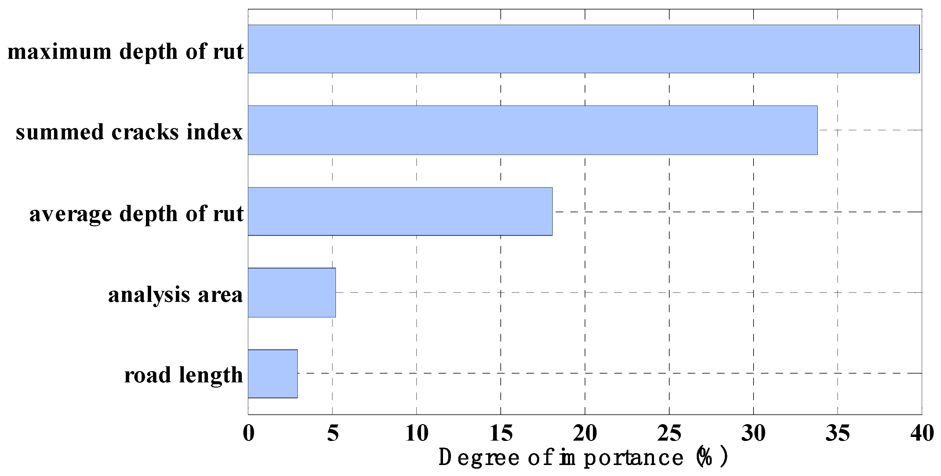
Data collection: in this step, the data generated from laboratory experiments were collected and summarized into two groups whereas the first groups contains all input parameters such as: road length, analysis area, summed cracks, maximum depth of rut, average depth of rut and the second one encloses the output parameter (IRI).

(ii)

Data pre-processing: in this step, PCA and the Savitzky–Golay filter were used to reduce the dimensions data and reduce extreme values in the distribution of data.

(iii)

Data preparation: in this study, the holdout validation method was used for training and validating the models as it is a popular and effective method for generating the datasets for training and testing the models [24,44,45,46,47,48,49,50,51,52,53,54,55,56,57,58,59,60,61], and thus the collected data were divided into two parts. The first part included 70% data which was used to train the models, whereas the second part contained 30%, the remaining data and this was used to validate the models as the ratio 70/30 for dividing the training and testing dataset was a common ratio used in applying the ML models [29,62,63,64,65,66,67,68,69,70,71].

(iv)

Training the models: the models were created using a 70% training dataset. PSOANFIS was created by combining PSO and ANFIS, GANFIS was created by combining GA and ANFIS, FAANFIS was created by combining FA and ANFIS. Out of these, PSO, GA, FA were used to optimize the consequence, antecedent parameters for giving the best ANFIS. An artificial neural network (ANN) was created using sigmoid algorithm.

(v)

Validation the models: after optimization of consequence, antecedent parameters, as well as training models, validation of the models were carried out using testing dataset via two methods namely RMSE and R.

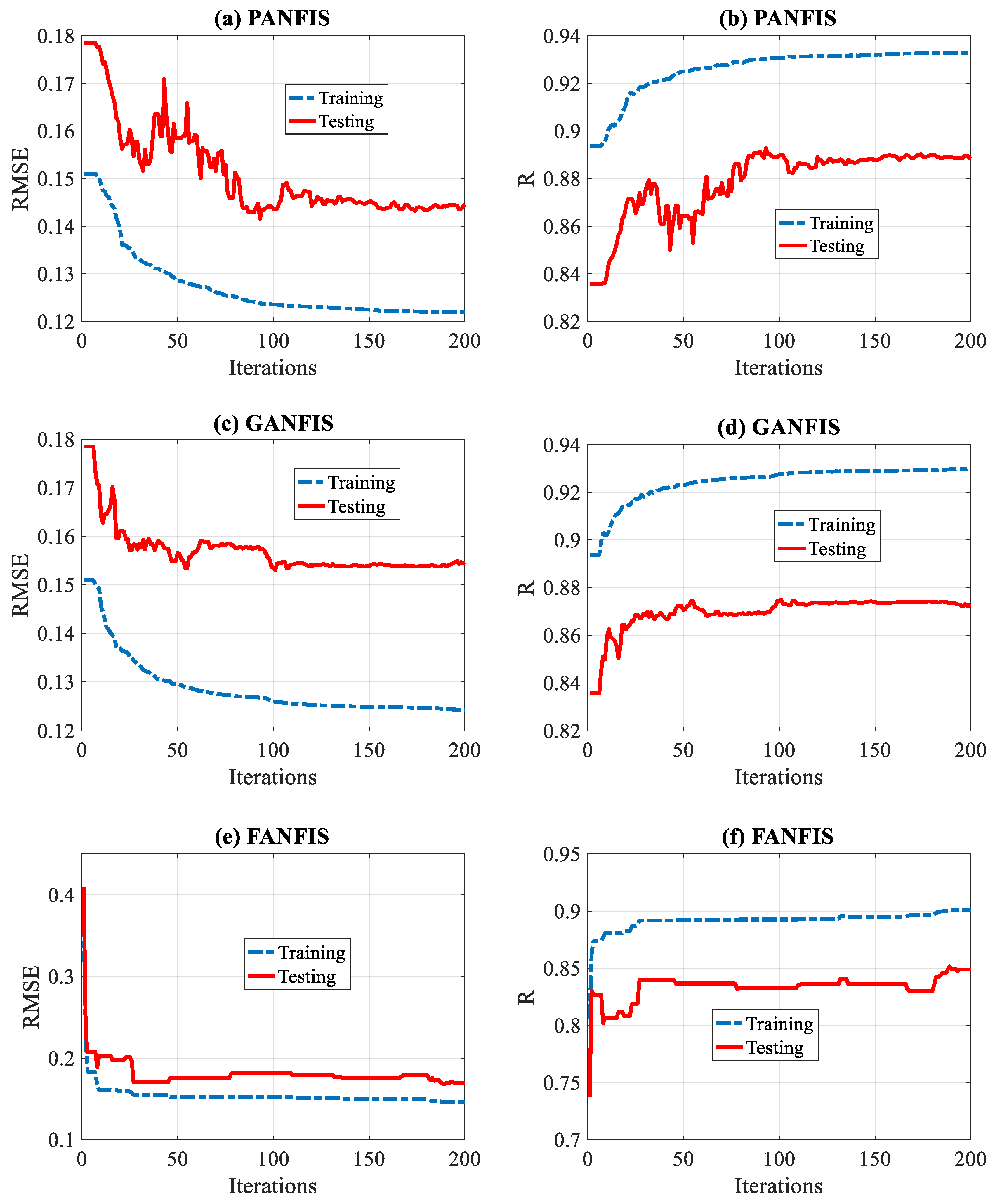
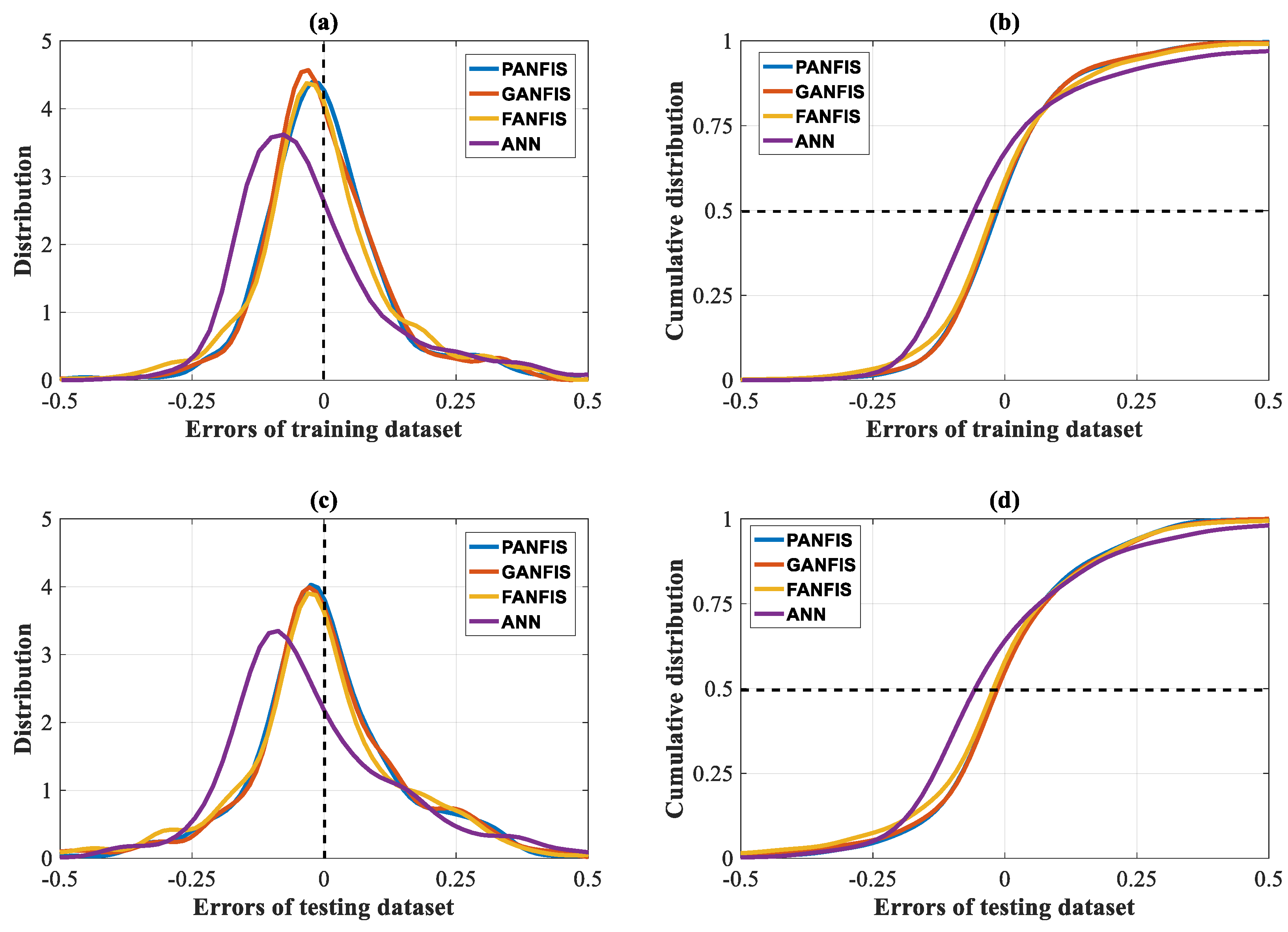
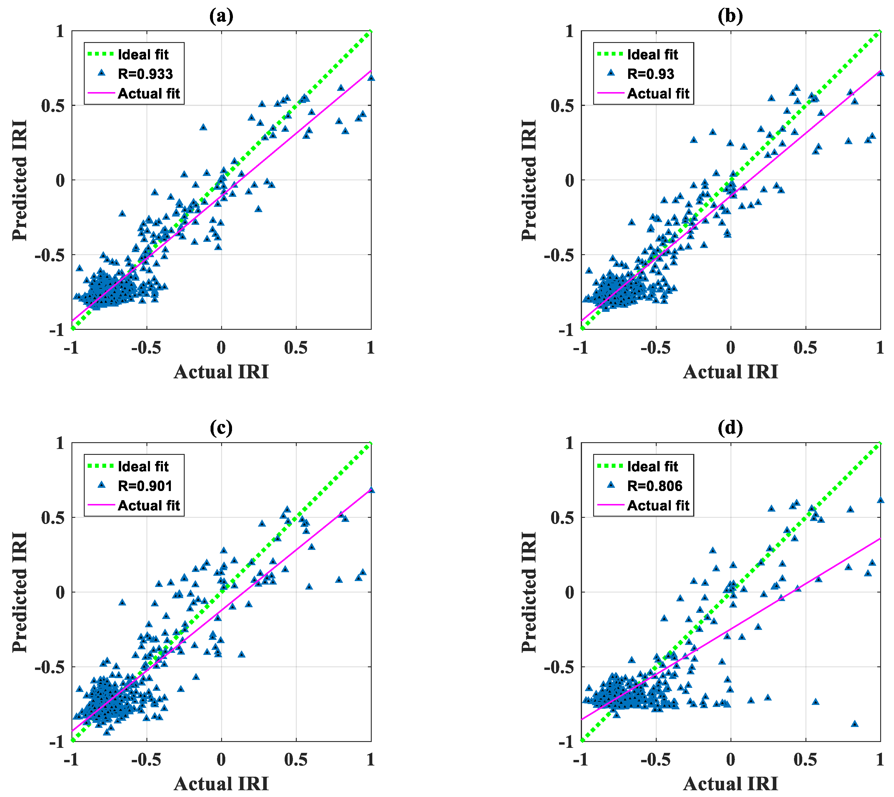
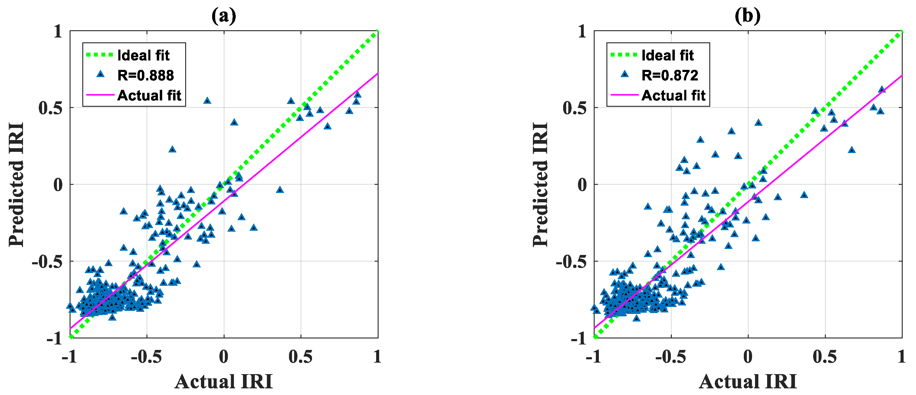
3. Results

Four ML models namely PSOANFIS, GANFIS, FAANFIS and ANN were constructed and trained for prediction of IRI. For PSOANFIS, GANFIS, and FAANFIS, an initial ANFIS structure was generated based on a number of membership functions. In the learning PSOANFIS, inertia weight, population size, personal learning coefficient and global learning coefficient were initially set as “0.4”, “100”, “1” and “2”, respectively, which achieved the best RMSE. In the learning GANFIS, crossover percentage, population size, mutation percentage, gamma and mutation rate were initially set as “0.4”, “100”, “0.7”, “0.7” and “0.15”, respectively. In the learning FAANFIS, initial parameters, namely the light absorption coefficient, attraction coefficient base value, and the mutation coefficient was selected as “1”, “2” and “0.2”, respectively. These hybrid models used RMSE criteria to validate the models for 200 iterations. In learning ANN, we constructed a network with 10 hidden neurons. In terms of a training network, the scaled conjugate gradient algorithm was used to find the bias and weight values of network. Figure 5 indicates cost functions in terms of RMSE and R when using PSO, GA and FA techniques for optimizing ANFIS parameters, respectively. It can be seen that 200 iterations were sufficient for achieving convergence of cost functions.

RMSE and errors were used to validate and compare models, and the results are illustrated in Figure 6. Summary information of RMSE and error mean and standard deviation are indicated in

Table 3. Summary of prediction capability of four artificial intelligence (AI) models.

Dataset	Model	RMSE	R	Slope	Error Mean	Error StD
Training dataset	PSOANFIS	0.122	0.933	0.838	0.004	0.122
	GANFIS	0.124	0.930	0.838	0.003	0.124
	FAANFIS	0.146	0.901	0.809	0.002	0.146
	Artificial neural networks (ANN)	0.200	0.806	0.607	0.000	0.200
Testing dataset	PSOANFIS	0.145	0.888	0.832	0.002	0.145
	GANFIS	0.155	0.872	0.823	0.000	0.155
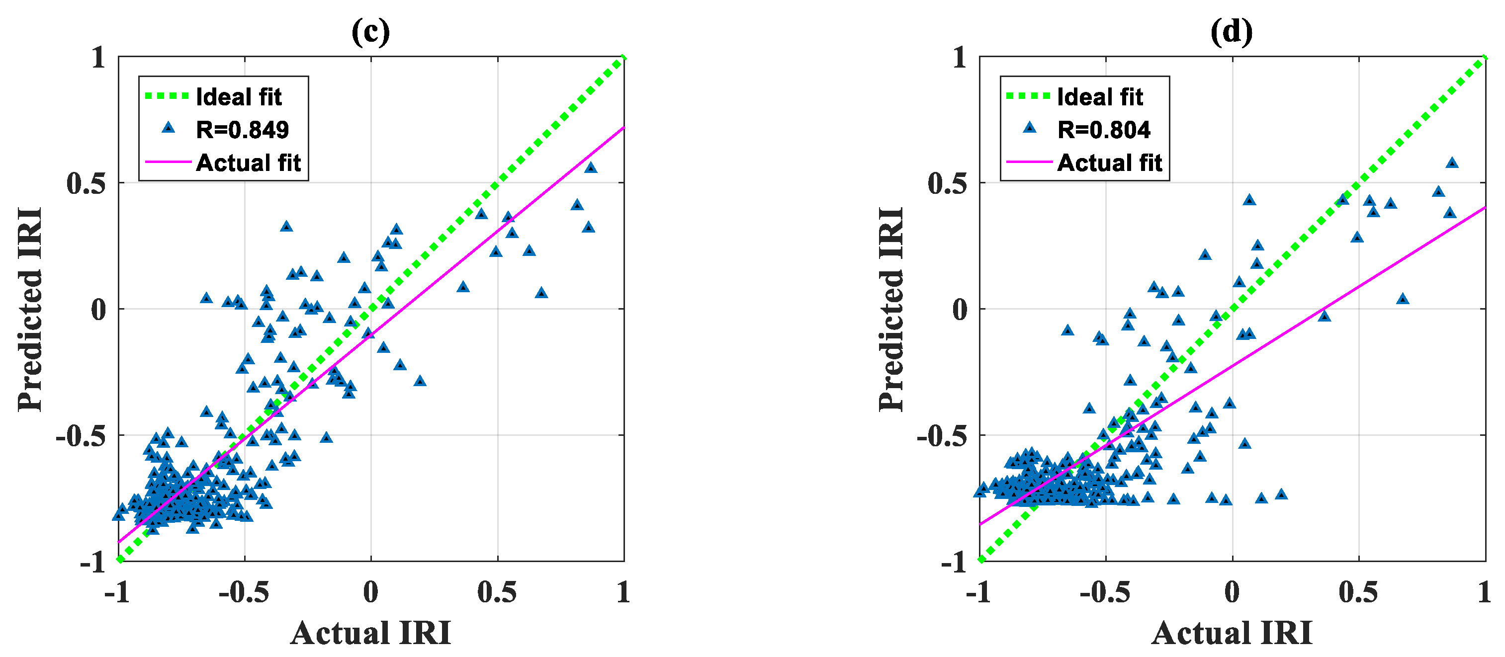
	FAANFIS	0.170	0.849	0.823	−0.010	0.170
	ANN	0.186	0.804	0.629	−0.009	0.187

A new hybrid approach between adaptive network based fuzzy inference system (ANFIS) and various meta-heuristic optimizations such as the genetic algorithm (GA), particle swarm optimization (PSO), and the firefly algorithm (FA) to develop several hybrid models namely GA based ANGIS (GANFIS), PSO based ANFIS (PSOANFIS), FA based ANFIS (FAANFIS).

. It shows that RMSE values of the models varied from 0.122 to 0.2 for the training dataset. In particular, the value of RMSE in PSOANFIS was lowest with 0.122, compared to 0.146, 0.124, 0.200 of the FAANFIS, GANFIS and ANN model, respectively. Thus, the PSOANFIS model had the best goodness of fit with training dataset in comparison with other models. Similarly, RMSE values of GANFIS, PSOANFIS, FAANFIS and ANN for testing dataset were 0.155, 0.145, 0.170 and 0.186, respectively, which also indicated that PSOANFIS had good performance in both the training dataset and the testing dataset compared to other models.

Validation of the models using the R criteria is shown in Figure 7 and Figure 8 for regression graphs between actual and predicted IRI. It can be observed from Figure 7 and Figure 8 that R values of four models varied from 0.806 to 0.933 for the training dataset. With R = 0.933, the PSOANFIS has the highest goodness of fit, followed by the GANFIS, FAANFIS, ANN with 0.930, 0.901, 0.806, respectively. For the testing dataset, the R values are 0.888 (PSOANFIS), 0.872 (GANFIS), 0.849 (FAANFIS) and 0.804 (ANN). Thus, in this study, PSOANFIS has a good prediction capability in both training dataset and testing dataset compared to other models.

Validation of statistical difference of the models using the Wilcoxon sign-ranked test was done as shown in

Table 4. Non-parametric test using training dataset.

No	Pair Samples	z-Value	p-Value	Significance
1	PSOANFIS vs. GANFIS	7.163	<0.0001	Yes
2	PSOANFIS vs. FAANFIS	−2.793	0.0052	Yes
3	PSOANFIS vs. ANN	−6.692	<0.0001	Yes
4	GANFIS vs. FAANFIS	−1.73	0.0836	No
5	GANFIS vs. ANN	−6.859	<0.0001	Yes
6	FAANFIS vs. ANN	−6.135	<0.0001	Yes

and

Table 5. Non-parametric test using testing dataset.

No	Pair Samples	z-Value	p-Value	Significance
1	PSOANFIS vs. GANFIS	6.35	<0.0001	Yes
2	PSOANFIS vs. FAANFIS	−3.997	0.0001	Yes
3	PSOANFIS vs. ANN	−5.597	<0.0001	Yes
4	GANFIS vs. FAANFIS	−2.869	0.0041	Yes
5	GANFIS vs. ANN	−5.897	<0.0001	Yes
6	FAANFIS vs. ANN	−4.2	<0.0001	Yes

. It can be observed in training dataset that p-value of the pair samples of the models is smaller than 0.05 except the pair sample of GANFIS vs. FAANFIS and the z-value of the pair samples of the models out of the range from −1.96 and +1.96 except the pair sample of GANFIS vs. FAANFIS (Table 4). In testing dataset, both p-value and z-values of all the pair samples of the models are less than 0.05 and out of the range from −1.96 and +1.96, respectively (Table 5). Therefore, it can be stated that in testing phase, the difference of all models is statistically significant whereas in training dataset the difference of the models is statistically significant except GANFIS vs. FAANFIS.

4. Discussion

Use of IRI has received much attention as a crucial tool for analysis of pavement performance prediction and life cycle cost because IRI is considered as a quality assurance parameter in the procedure of construction [72] and reflects the ride quality and comfort level of passengers. Besides, roughness-based indices have been used as a practical and reliable method for predicting performance of pavement and analyzing maintenance and rehabilitation [73]. The health status of the pavement can be assessed by observing present distresses, checking the material properties and estimating quality of the construction [74]. As assessment of the performance of the road pavement structure based on IRI prediction is a very important and necessary task for efficient management of the road infrastructure, there are several studies on the relationship between IRI and pavement distress [75,76,77]. Determination of IRI is important task to quantify road surface roughness. On the other hand, the traditional methods to measure the IRI is time-consuming and cost a great fee. Thus, prediction of the IRI using advanced ML techniques is an effective solution which has not only a quick determination but also reduces significantly the cost of measurement. In the present study, we recommended potential ML methods PSOANFIS, GANFIS, FAANFIS, and ANN which have a better prediction capability for the IRI.

It can be observed from the validation results of the models that the PSOANFIS, GANFIS, FAANFIS model have acceptable performance whereas ANN has a slightly poor capability for the prediction of the IRI. It can be stated that PSOANFIS has stable performance and the best prediction capability, followed by GANFIS, the FAANFIS and the ANN (Figure 5, Figure 6, Figure 7 and Figure 8 and Table 3, Table 4 and Table 5). It is because the GANFIS, PSOANFIS, FAANFIS used the GA, PSO, FA to optimize parameters, thereby reducing the error of prediction. The calculation of these methods is very simple, occupies the bigger optimization ability and can be completed easily. Although ML methods such as PSOANFIS, GANFIS, FAANFIS, ANN has a great potentiality for prediction problems, their predictive capability depends substantial on the quality of dataset. In term of prediction problems, the variables used have determination from various experiments on various sample can have effect on the predictive capability of the models. To improve the capability of the ML models, one of many solutions is that it needs to be provided more numbers of data. In this study, four potential ML techniques have low average error rates, so that it might be used to predict other properties of the road surface.

In applying ML models, it is essential to carry out the sensitivity analysis to evaluate the importance of the input parameters used for training and validating the models. Thus, in the present study, a sensitivity analysis was carried out for estimating the degree of importance of each input variable on the prediction of IRI. The sensitivity analysis was calculated using the PSOANFIS model, as its prediction capability has been proved as the best. For this purpose, quantile values at 21 points (from 0 to 1 with a resolution of 0.05) of each input have been extracted and served as a new dataset for the calculation of IRI through the PSOANFIS model. In order to explore the sensitivity, each input was varied from its smallest (quantile 0) to biggest (quantile 1) values while all other variables remained at their median (quantile 0.5). Therefore, the normalized change in IRI output results could be used to quantify the degree of importance of input variables. Such calculation could be expressed by the following equation for computing the normalized change ϕ in IRI output results:

$${\phi }_i^j=\frac{{IRI}_i^j-{IRI}_{quantile-0.5}^{all-inputs}}{{IRI}_{quantile-0.5}^{all-inputs}}$$

(12)

where ${IRI}_{quantile-0.5}^{all-inputs}$ was the configuration “zero” when all inputs remained at their medians, ${IRI}_i^j$ is the IRI output results using jth input at its ith quantile level. In this work, quantile level varies from 0 to 1 with a resolution of 0.05 (i = 1, …, 21). Finally, the degree of importance of each input was calculated based on the following equation:

$${\mathsf{\Phi }}^i={\displaystyle \sum _{i=1}^{21}}{\phi }_i^j$$

(13)

Indeed, such variation in statistical behavior of inputs allows efficiently computing their influence in the prediction of IRI. Results of sensitivity analysis are scaled into the range of [0, 100%] and plotted in Figure 9 in the descending order. Obviously, all inputs exhibited impact on the prediction of IRI through the PSOANFIS model. However, the most influenced variables were maximum depth of rut, summed cracks and average depth of rut, which exposed 40, 34 and 17% of degree of importance, respectively. The other two inputs such as analysis area and road length exhibited less than 9% of degree of importance. Such obtained information was relevant and could help engineers save time and cost in applications and practices. The results of this sensitivity analysis might be helpful in selection of suitable input parameters for better performance of ML models for prediction of IRI and other properties of road surface.

5. Conclusions

Prediction of IRI is an important task in quantification road surface roughness. In the present study, we proposed an efficient approach using hybrid ML models such as PSOANFIS, GANFIS, FAANFIS which was also compared with a benchmark ML model named ANN. Data were provided from the survey area in the north of Vietnam. PSOANFIS, GANFIS, FAANFIS are hybrid models of ANFIS optimized by three meta-heuristic optimization algorithm; PSO, GA and FA. Experimental results performed on ML algorithms illustrated that PSOANFIS had the best capability in prediction compared to other applied models. The sensitivity analysis results showed that the most important parameters, namely maximum depth of rut, summed cracks and average depth of rut, should be taken into account in predicting IRI using the ML models. Results of this study were helpful for engineers and researchers to predict quickly and accurately the IRI for evaluating and managing road systems. It will also help to reduce the cost due to reduction of the cost of laboratorial experiments. However, it was noticed that cross-validation is also an effective method to validate the performance of the ML models, which can be investigated in further study instead of the holdout validation used in this study. In addition, other less biased ML techniques such as random forest should be used to compare with the proposed and applied models of this study for future works.

References

- Arhin, S.A.; Williams, L.N.; Ribbiso, A.; Anderson, M.F. Predicting pavement condition index using international roughness index in a dense urban area. J. Civ. Eng. Res. 2015, 5, 10–17. [Google Scholar]
- Li, J.; Zhang, Z.; Wang, W. International roughness index and a new solution for its calculation. J. Transp. Eng. Part B Pavements 2018, 144, 06018002. [Google Scholar] [CrossRef]
- Hossain, M.; Gopisetti, L.; Miah, M. International Roughness Index Prediction of Flexible Pavements Using Neural Networks. J. Transp. Eng. Part B Pavements 2018, 145, 04018058. [Google Scholar] [CrossRef]
- Ziari, H.; Sobhani, J.; Ayoubinejad, J.; Hartmann, T. Prediction of IRI in short and long terms for flexible pavements: ANN and GMDH methods. Int. J. Pavement Eng. 2016, 17, 776–788. [Google Scholar] [CrossRef]
- Khalifeh, V.; Golroo, A.; Ovaici, K. Application of an Inexpensive Sensor in Calculating the International Roughness Index. J. Comput. Civ. Eng. 2018, 32, 04018022. [Google Scholar] [CrossRef]
- Chen, C.-T.; Hung, C.-T.; Chou, C.-C.; Chiang, Z.; Lin, J.-D. The predicted model of international roughness index for drainage asphalt pavement. In Proceedings of the International Conference on Intelligent Computing, Shanghai, China, 15–18 September 2008; pp. 937–945. [Google Scholar]
- Lin, J.-D.; Yau, J.-T.; Hsiao, L.-H. Correlation analysis between international roughness index (IRI) and pavement distress by neural network. In Proceedings of the 82th Annual Meeting of the Transportation Research Board, Washington, DC, USA, 12–16 January 2003; pp. 12–16. [Google Scholar]
- Yousefzadeh, M.; Azadi, S.; Soltani, A. Road profile estimation using neural network algorithm. J. Mech. Sci. Technol. 2010, 24, 743–754. [Google Scholar] [CrossRef]
- Mactutis, J.A.; Alavi, S.H.; Ott, W.C. Investigation of relationship between roughness and pavement surface distress based on WesTrack project. Transp. Res. Rec. 2000, 1699, 107–113. [Google Scholar] [CrossRef]
- Wold, S.; Esbensen, K.; Geladi, P. Principal component analysis. Chemom. Intell. Lab. Syst. 1987, 2, 37–52. [Google Scholar] [CrossRef]
- Press, W.H.; Teukolsky, S.A. Savitzky-Golay smoothing filters. Comput. Phys. 1990, 4, 669–672. [Google Scholar] [CrossRef]
- Le, L.M.; Ly, H.-B.; Pham, B.T.; Le, V.M.; Pham, T.A.; Nguyen, D.-H.; Tran, X.-T.; Le, T.-T. Hybrid Artificial Intelligence Approaches for Predicting Buckling Damage of Steel Columns under Axial Compression. Materials 2019, 12, 1670. [Google Scholar] [CrossRef]
- Ly, H.-B.; Le, L.M.; Duong, H.T.; Nguyen, T.C.; Pham, T.A.; Le, T.-T.; Le, V.M.; Nguyen-Ngoc, L.; Pham, B.T. Hybrid Artificial Intelligence Approaches for Predicting Critical Buckling Load of Structural Members under Compression Considering the Influence of Initial Geometric Imperfections. Appl. Sci. 2019, 9, 2258. [Google Scholar] [CrossRef]
- Termeh, S.V.R.; Khosravi, K.; Sartaj, M.; Keesstra, S.D.; Tsai, F.T.-C.; Dijksma, R.; Pham, B.T. Optimization of an adaptive neuro-fuzzy inference system for groundwater potential mapping. Hydrogeol. J. 2019, 27, 2511–2534. [Google Scholar] [CrossRef]
- Manogaran, G.; Varatharajan, R.; Priyan, M. Hybrid recommendation system for heart disease diagnosis based on multiple kernel learning with adaptive neuro-fuzzy inference system. Multimed. Tools Appl. 2018, 77, 4379–4399. [Google Scholar] [CrossRef]
- Marini, F.; Walczak, B. Particle swarm optimization (PSO). A tutorial. Chemom. Intell. Lab. Syst. 2015, 149, 153–165. [Google Scholar] [CrossRef]
- Eberhart, R.; Kennedy, J. Particle swarm optimization. In Proceedings of the IEEE International Conference on Neural Networks, Budapest, Hungary, 14–19 July 2019; pp. 1942–1948. [Google Scholar]
- Du, K.-L.; Swamy, M. Particle swarm optimization. In Search and Optimization by Metaheuristics; Springer: Basel, Switzerland, 2016; pp. 153–173. [Google Scholar]
- Chatterjee, S.; Sarkar, S.; Hore, S.; Dey, N.; Ashour, A.S.; Balas, V.E. Particle swarm optimization trained neural network for structural failure prediction of multistoried RC buildings. Neural Comput. Appl. 2017, 28, 2005–2016. [Google Scholar] [CrossRef]
- Juang, C.-F. A hybrid of genetic algorithm and particle swarm optimization for recurrent network design. IEEE Trans. Syst. Man Cybern. Part B (Cybernetics) 2004, 34, 997–1006. [Google Scholar] [CrossRef]
- Gai, K.; Qiu, M.; Zhao, H. Cost-aware multimedia data allocation for heterogeneous memory using genetic algorithm in cloud computing. IEEE Trans. Cloud Comput. 2016. [Google Scholar] [CrossRef]
- Mitchell, M. An Introduction to Genetic Algorithms; MIT Press: Cambridge, UK, 1998. [Google Scholar]
- Yang, X. Firefly Algorithm, Nature Inspired Metaheuristic Algorithms, 2010; Luniver Press: Frome, UK, 2010. [Google Scholar]
- Bayat, M.; Ghorbanpour, M.; Zare, R.; Jaafari, A.; Pham, B.T. Application of artificial neural networks for predicting tree survival and mortality in the Hyrcanian forest of Iran. Comput. Electron. Agric. 2019, 164, 104929. [Google Scholar] [CrossRef]
- Hassoun, M.H. Fundamentals of Artificial Neural Networks; MIT Press: Cambridge, UK, 1995. [Google Scholar]
- Basheer, I.A.; Hajmeer, M. Artificial neural networks: Fundamentals, computing, design, and application. J. Microbiol. Methods 2000, 43, 3–31. [Google Scholar] [CrossRef]
- Apostolopoulou, M.; Armaghani, D.J.; Bakolas, A.; Douvika, M.G.; Moropoulou, A.; Asteris, P.G. Compressive strength of natural hydraulic lime mortars using soft computing techniques. Procedia Struct. Integr. 2019, 17, 914–923. [Google Scholar] [CrossRef]
- Armaghani, D.J.; Hatzigeorgiou, G.D.; Karamani, C.; Skentou, A.; Zoumpoulaki, I.; Asteris, P.G. Soft computing-based techniques for concrete beams shear strength. Procedia Struct. Integr. 2019, 17, 924–933. [Google Scholar] [CrossRef]
- Khozani, Z.S.; Khosravi, K.; Pham, B.T.; Kløve, B.; Mohtar, W.; Melini, W.H.; Yaseen, Z.M. Determination of compound channel apparent shear stress: Application of novel data mining models. J. Hydroinform. 2019, 21, 798–811. [Google Scholar] [CrossRef]
- Pham, B.T.; Nguyen, M.D.; Van Dao, D.; Prakash, I.; Ly, H.-B.; Le, T.-T.; Ho, L.S.; Nguyen, K.T.; Ngo, T.Q.; Hoang, V. Development of artificial intelligence models for the prediction of Compression Coefficient of soil: An application of Monte Carlo sensitivity analysis. Sci. Total Environ. 2019, 679, 172–184. [Google Scholar] [CrossRef] [PubMed]
- Chen, H.; Asteris, P.G.; Jahed Armaghani, D.; Gordan, B.; Pham, B.T.J.A.S. Assessing dynamic conditions of the retaining wall: developing two hybrid intelligent models. Appl. Sci. 2019, 9, 1042. [Google Scholar] [CrossRef]
- Nguyen, H.-L.; Le, T.-H.; Pham, C.-T.; Le, T.-T.; Ho, L.S.; Le, V.M.; Pham, B.T.; Ly, H.-B. Development of Hybrid Artificial Intelligence Approaches and a Support Vector Machine Algorithm for Predicting the Marshall Parameters of Stone Matrix Asphalt. Appl. Sci. 2019, 9, 3172. [Google Scholar] [CrossRef]
- Ly, H.-B.; Desceliers, C.; Le, L.M.; Le, T.-T.; Pham, B.T.; Nguyen-Ngoc, L.; Doan, V.T.; Le, M. Quantification of Uncertainties on the Critical Buckling Load of Columns under Axial Compression with Uncertain Random Materials. Materials 2019, 12, 1828. [Google Scholar] [CrossRef]
- Nakagawa, S.; Johnson, P.C.; Schielzeth, H. The coefficient of determination R2 and intra-class correlation coefficient from generalized linear mixed-effects models revisited and expanded. J. R. Soc. Interface 2017, 14. [Google Scholar] [CrossRef]
- Ly, H.-B.; Monteiro, E.; Le, T.-T.; Le, V.M.; Dal, M.; Regnier, G.; Pham, B.T. Prediction and sensitivity analysis of bubble dissolution time in 3D selective laser sintering using ensemble decision trees. Materials 2019, 12, 1544. [Google Scholar] [CrossRef]
- Dao, D.V.; Ly, H.-B.; Trinh, S.H.; Le, T.-T.; Pham, B.T. Artificial intelligence approaches for prediction of compressive strength of geopolymer concrete. Materials 2019, 12, 983. [Google Scholar] [CrossRef]
- Dao, D.V.; Trinh, S.H.; Ly, H.-B.; Pham, B.T. Prediction of compressive strength of geopolymer concrete using entirely steel slag aggregates: Novel hybrid artificial intelligence approaches. Appl. Sci. 2019, 9, 1113. [Google Scholar] [CrossRef]
- Nagelkerke, N.J. A note on a general definition of the coefficient of determination. Biometrika 1991, 78, 691–692. [Google Scholar] [CrossRef]
- Chai, T.; Draxler, R.R. Root mean square error (RMSE) or mean absolute error (MAE)?—Arguments against avoiding RMSE in the literature. Geosci. Model Dev. 2014, 7, 1247–1250. [Google Scholar] [CrossRef]
- Asteris, P.G.; Kolovos, K.G. Self-compacting concrete strength prediction using surrogate models. Neural Comput. Appl. 2019, 31, 409–424. [Google Scholar] [CrossRef]
- Sarir, P.; Chen, J.; Asteris, P.G.; Armaghani, D.J.; Tahir, M. Developing GEP tree-based, neuro-swarm, and whale optimization models for evaluation of bearing capacity of concrete-filled steel tube columns. Eng. Comput. 2019, 1–19. [Google Scholar] [CrossRef]
- Bui, D.T.; Shirzadi, A.; Shahabi, H.; Chapi, K.; Omidavr, E.; Pham, B.T.; Asl, D.T.; Khaledian, H.; Pradhan, B.; Panahi, M. A Novel Ensemble Artificial Intelligence Approach for Gully Erosion Mapping in a Semi-Arid Watershed (Iran). Sensors 2019, 19, 2444. [Google Scholar] [CrossRef]
- Bui, D.T.; Tuan, T.A.; Klempe, H.; Pradhan, B.; Revhaug, I. Spatial prediction models for shallow landslide hazards: A comparative assessment of the efficacy of support vector machines, artificial neural networks, kernel logistic regression, and logistic model tree. Landslides 2016, 13, 361–378. [Google Scholar]
- Pham, B.T.; Nguyen, M.D.; Ly, H.-B.; Pham, T.A.; Hoang, V.; Van Le, H.; Le, T.-T.; Nguyen, H.Q.; Bui, G.L. Development of Artificial Neural Networks for Prediction of Compression Coefficient of Soft Soil. In CIGOS 2019, Innovation for Sustainable Infrastructure; Springer: Singapore, 2020; pp. 1167–1172. [Google Scholar]
- Le, T.-T.; Pham, B.T.; Ly, H.-B.; Shirzadi, A.; Le, L.M. Development of 48-hour Precipitation Forecasting Model using Nonlinear Autoregressive Neural Network. In CIGOS 2019, Innovation for Sustainable Infrastructure; Springer: Singapore, 2020; pp. 1191–1196. [Google Scholar]
- Thanh, T.T.M.; Ly, H.-B.; Pham, B.T. A Possibility of AI Application on Mode-choice Prediction of Transport Users in Hanoi. In CIGOS 2019, Innovation for Sustainable Infrastructure; Springer: Singapore, 2020; pp. 1179–1184. [Google Scholar]
- Khosravi, K.; Daggupati, P.; Alami, M.T.; Awadh, S.M.; Ghareb, M.I.; Panahi, M.; Pham, B.T.; Rezaie, F.; Qi, C.; Yaseen, Z.M. Meteorological data mining and hybrid data-intelligence models for reference evaporation simulation: A case study in Iraq. Comput. Electron. Agric. 2019, 167, 105041. [Google Scholar] [CrossRef]
- Pham, B.T.; Jaafari, A.; Prakash, I.; Singh, S.K.; Quoc, N.K.; Bui, D.T. Hybrid computational intelligence models for groundwater potential mapping. Catena 2019, 182, 104101. [Google Scholar] [CrossRef]
- Phong, T.V.; Phan, T.T.; Prakash, I.; Singh, S.K.; Shirzadi, A.; Chapi, K.; Ly, H.-B.; Ho, L.S.; Quoc, N.K.; Pham, B.T. Landslide susceptibility modeling using different artificial intelligence methods: A case study at Muong Lay district, Vietnam. Geocarto Int. 2019. [Google Scholar] [CrossRef]
- Nguyen, M.D.; Pham, B.T.; Tuyen, T.T.; Yen, H.; Phan, H.; Prakash, I.; Vu, T.T.; Chapi, K.; Shirzadi, A.; Shahabi, H. Development of an Artificial Intelligence Approach for Prediction of Consolidation Coefficient of Soft Soil: A Sensitivity Analysis. Open Constr. Build. Technol. J. 2019, 13, 178–188. [Google Scholar] [CrossRef]
- Chang, K.-T.; Merghadi, A.; Yunus, A.P.; Pham, B.T.; Dou, J. Evaluating scale effects of topographic variables in landslide susceptibility models using GIS-based machine learning techniques. Sci. Rep. 2019, 9, 12296. [Google Scholar] [CrossRef] [PubMed]
- Nohani, E.; Moharrami, M.; Sharafi, S.; Khosravi, K.; Pradhan, B.; Pham, B.T.; Lee, S.; M Melesse, A. Landslide susceptibility mapping using different GIS-based bivariate models. Water 2019, 11, 1402. [Google Scholar] [CrossRef]
- Pham, B.T.; Prakash, I.; Jaafari, A.; Bui, D.T. Spatial prediction of rainfall-induced landslides using aggregating one-dependence estimators classifier. J. Indian Soc. Remote Sens. 2018, 46, 1457–1470. [Google Scholar] [CrossRef]
- Abedini, M.; Ghasemian, B.; Shirzadi, A.; Shahabi, H.; Chapi, K.; Pham, B.T.; Bin Ahmad, B.; Tien Bui, D. A novel hybrid approach of bayesian logistic regression and its ensembles for landslide susceptibility assessment. Geocarto Int. 2018, 34, 1427–1457. [Google Scholar] [CrossRef]
- Pham, B.T. A novel classifier based on composite hyper-cubes on iterated random projections for assessment of landslide susceptibility. J. Geol. Soc. India 2018, 91, 355–362. [Google Scholar] [CrossRef]
- Jaafari, A.; Zenner, E.K.; Pham, B.T. Wildfire spatial pattern analysis in the Zagros Mountains, Iran: A comparative study of decision tree based classifiers. Ecol. Inform. 2018, 43, 200–211. [Google Scholar] [CrossRef]
- Pham, B.T.; Prakash, I. Spatial prediction of rainfall induced shallow landslides using adaptive-network-based fuzzy inference system and particle swarm optimization: A case study at the Uttarakhand Area, India. In Proceedings of the International Conference on Geo-Spatial Technologies and Earth Resources, Hanoi, Vietnam, 5–6 October 2017; pp. 224–238. [Google Scholar]
- Pham, B.T.; Prakash, I. A Novel Hybrid Intelligent Approach of Random Subspace Ensemble and Reduced Error Pruning Trees for Landslide Susceptibility Modeling: A Case Study at Mu Cang Chai District, Yen Bai Province, Viet Nam. In Proceedings of the International Conference on Geo-Spatial Technologies and Earth Resources, Hanoi, Vietnam, 5–6 October 2017; pp. 255–269. [Google Scholar]
- Pham, B.T.; Nguyen, V.-T.; Ngo, V.-L.; Trinh, P.T.; Ngo, H.T.T.; Bui, D.T. A novel hybrid model of rotation forest based functional trees for landslide susceptibility mapping: A case study at Kon Tum Province, Vietnam. In Proceedings of the International Conference on Geo-Spatial Technologies and Earth Resources, Hanoi, Vietnam, 5–6 October 2017; pp. 186–201. [Google Scholar]
- Khosravi, K.; Sartaj, M.; Tsai, F.T.-C.; Singh, V.P.; Kazakis, N.; Melesse, A.M.; Prakash, I.; Bui, D.T.; Pham, B.T. A comparison study of DRASTIC methods with various objective methods for groundwater vulnerability assessment. Sci. Total Environ. 2018, 642, 1032–1049. [Google Scholar] [CrossRef]
- Miraki, S.; Zanganeh, S.H.; Chapi, K.; Singh, V.P.; Shirzadi, A.; Shahabi, H.; Pham, B.T. Mapping groundwater potential using a novel hybrid intelligence approach. Water Resour. Manag. 2019, 33, 281–302. [Google Scholar] [CrossRef]
- Dou, J.; Yunus, A.P.; Xu, Y.; Zhu, Z.; Chen, C.-W.; Sahana, M.; Khosravi, K.; Yang, Y.; Pham, B.T. Torrential rainfall-triggered shallow landslide characteristics and susceptibility assessment using ensemble data-driven models in the Dongjiang Reservoir Watershed, China. Nat. Hazards 2019, 97, 579–609. [Google Scholar] [CrossRef]
- Khosravi, K.; Shahabi, H.; Pham, B.T.; Adamowski, J.; Shirzadi, A.; Pradhan, B.; Dou, J.; Ly, H.-B.; Gróf, G.; Ho, H.L. A comparative assessment of flood susceptibility modeling using Multi-Criteria Decision-Making Analysis and Machine Learning Methods. J. Hydrol. 2019, 573, 311–323. [Google Scholar] [CrossRef]
- Pham, B.T.; Prakash, I. Evaluation and comparison of LogitBoost Ensemble, Fisher’s Linear Discriminant Analysis, logistic regression and support vector machines methods for landslide susceptibility mapping. Geocarto Int. 2019, 34, 316–333. [Google Scholar] [CrossRef]
- Nguyen, V.V.; Pham, B.T.; Vu, B.T.; Prakash, I.; Jha, S.; Shahabi, H.; Shirzadi, A.; Ba, D.N.; Kumar, R.; Chatterjee, J.M. Hybrid machine learning approaches for landslide susceptibility modeling. Forests 2019, 10, 157. [Google Scholar] [CrossRef]
- Pham, B.T.; Nguyen, M.D.; Bui, K.-T.T.; Prakash, I.; Chapi, K.; Bui, D.T. A novel artificial intelligence approach based on Multi-layer Perceptron Neural Network and Biogeography-based Optimization for predicting coefficient of consolidation of soil. Catena 2019, 173, 302–311. [Google Scholar] [CrossRef]
- Janizadeh, S.; Avand, M.; Jaafari, A.; Phong, T.V.; Bayat, M.; Ahmadisharaf, E.; Prakash, I.; Pham, B.T.; Lee, S. Prediction Success of Machine Learning Methods for Flash Flood Susceptibility Mapping in the Tafresh Watershed, Iran. Sustainability 2019, 11, 5426. [Google Scholar] [CrossRef]
- Pham, B.T.; Shirzadi, A.; Shahabi, H.; Omidvar, E.; Singh, S.K.; Sahana, M.; Asl, D.T.; Ahmad, B.B.; Quoc, N.K.; Lee, S. Landslide susceptibility assessment by novel hybrid machine learning algorithms. Sustainability 2019, 11, 4386. [Google Scholar] [CrossRef]
- Dou, J.; Yunus, A.P.; Bui, D.T.; Sahana, M.; Chen, C.-W.; Zhu, Z.; Wang, W.; Pham, B.T. Evaluating GIS-Based Multiple Statistical Models and Data Mining for Earthquake and Rainfall-Induced Landslide Susceptibility Using the LiDAR DEM. Remote Sens. 2019, 11, 638. [Google Scholar] [CrossRef]
- Jaafari, A.; Mafi-Gholami, D.; Thai Pham, B.; Tien Bui, D. Wildfire Probability Mapping: Bivariate vs. Multivariate Statistics. Remote Sens. 2019, 11, 618. [Google Scholar] [CrossRef]
- Dou, J.; Yunus, A.P.; Bui, D.T.; Merghadi, A.; Sahana, M.; Zhu, Z.; Chen, C.-W.; Khosravi, K.; Yang, Y.; Pham, B.T. Assessment of advanced random forest and decision tree algorithms for modeling rainfall-induced landslide susceptibility in the Izu-Oshima Volcanic Island, Japan. Sci. Total Environ. 2019, 662, 332–346. [Google Scholar] [CrossRef]
- Al-Omari, B.; Darter, M. Effect of Pavement Deterioration Types on IRI and Rehabilitation; Transportation Research Record 1505; TRB: Washington, DC, USA, 1995. [Google Scholar]
- Park, K.; Thomas, N.E.; Wayne Lee, K.J.J.O.T.E. Applicability of the international roughness index as a predictor of asphalt pavement condition. J. Transp. Eng. 2007, 133, 706–709. [Google Scholar] [CrossRef]
- Mazari, M.; Rodriguez, D.D. Prediction of pavement roughness using a hybrid gene expression programming-neural network technique. J. Traffic Transp. Eng. 2016, 3, 448–455. [Google Scholar] [CrossRef] [Green Version]
- Prasad, J.R.; Kanuganti, S.; Bhanegaonkar, P.N.; Sarkar, A.K.; Arkatkar, S. Development of Relationship between Roughness (IRI) and Visible Surface Distresses: A Study on PMGSY Roads. Procedia Soc. Behav. Sci. 2013, 104, 322–331. [Google Scholar] [CrossRef] [Green Version]
- Chandra, S.; Sekhar, C.R.; Bharti, A.K.; Kangadurai, B. Relationship between Pavement Roughness and Distress Parameters for Indian Highways. J. Transp. Eng. 2013, 139, 467–475. [Google Scholar] [CrossRef]
- Sandra, A.K.; Sarkar, A.K. Development of a model for estimating International Roughness Index from pavement distresses. Int. J. Pavement Eng. 2013, 14, 715–724. [Google Scholar] [CrossRef]