1. Introduction
Logistics centers are common in cities where the balance between the transportation costs (from the producers to the consumers), storage costs, and other factors make its implementation viable. The energy consumption for the preservation of perishable foods, waste disposal, air conditioning, space, and parking lighting represent a relevant share of their total costs.
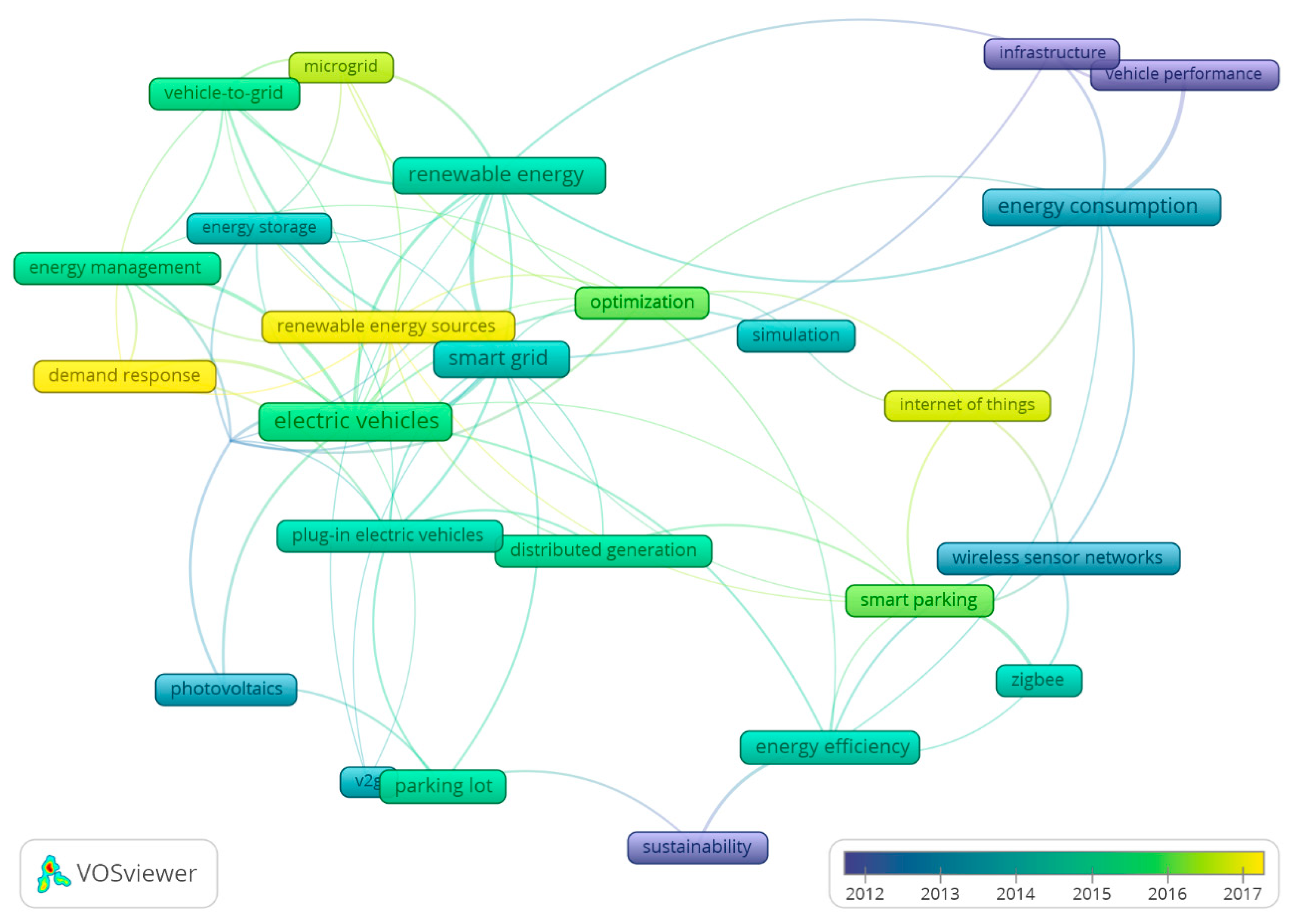
Regarding the interest in this topic, we accessed the Elsevier Scopus scientific database [
1]. Keywords related to this study were selected and a search investigated the documents’ fields titles, abstracts, and keywords in order to retrieve the most relevant publications. The Boolean combination of keywords (“Energy Efficiency” OR “Energy Consumption” OR “Renewable Energy” OR “Solar Energy” AND “Logistics Center” OR “Logistics Centre” OR “Parking”) resulted in a set of 544 documents published since 1975 to the present. These documents were categorized into five clusters using VOSviewer Bibliometric Software [
2], according to the occurrence frequency of 1289 author keywords, to envisage the main concerns and findings of the academic community related to this sector.
Figure 1 shows these main concerns in the most recent publications.
Each of these clusters can shed some light on the main problems and innovations in energy efficiency, as related to the logistics center sector.
Recently, the demand response, which consists of load shifting and the peak shaving of energy demand aiming for the lowest energy tariffs, the integration of distributed generated energy (PV) through smart grids with infrastructure demands, and electric vehicle supply are some of the most discussed issues.
Zadek and Schulz [
3] discussed the sustainability aspects of logistics centers by emphasizing technologies using local renewable energy sources (PV) to supply the infrastructure and transportation demands including hydrogen (
) production for their forklifts. Bradshaw and David [
4] showed how a technologically advanced workplace was helping to reduce environmental impact and lower operating costs by using green building elements such as PVs, a grey-water recycling system, and energy-efficient lighting.
Honarmand et al. [
5] proposed an energy resource management model for a microgrid in parking, arguing in favor of the integration of electric vehicles (EV) and the renewable energy source (PV), thus balancing the intermittent nature of PV generation and the uncontrolled charging/discharging procedure of EVs. Along the same line, Tulpule et al. [
6] also studied the economic and environmental impacts of PV powered parking with charging station for EVs. Rahmani-Andebili [
7] studied the impacts of canopying EV parking lots with PV panels.
The use of the Internet of Things (IoT) and wireless sensor networks (WSN) are also evident. For example, Yang [
8] studied the connectionless indoor inventory tracking sensor network in logistics centers using an open-source communication protocol for monitoring and control, named Zigbee RFID (Radio Frequency Identification). The use of WSN in buildings and warehouses for temperature measurements, motion sensing in lighting and ventilation systems are also some applications with an energy-saving purpose, as discussed by studies by Seo et al. [
9], Chang et al. [
10], and Cho et al. [
11].
The use of renewable energy sources, mainly PVs connected to the grid and associated with batteries, were analyzed by Dávi et al. [
12], where they discussed the advantages and the restrictions that influenced the feasibility of its implementation using modeling in an EnergyPlus environment. Along the same line, Kies et al. [
13] studied the use of PVs and batteries that were not connected to the grid.
Concerning the use of simulation tools for the calculation of PV solutions, the use of TRNSYS can be found in the studies of Villa-Arrieta and Sumper [
14], linking the technical and economic variables. Additionally, Antoniadis and Martinopoulos [
15] used this approach to optimize a solar thermal system.
The publications above-mentioned have made it possible to verify that energy efficiency studies for buildings using TRNSYS have been well addressed in academia, although the most common modeling solutions are based on theoretical constructs or prototypes.
The novelty of this article remains the use of a methodology that connects TRNSYS and other programs to optimize all of the decision variables that are based on a real-life case study.
During the optimizations, we approached the issue of surplus energy, which can occur with the installation of panels beside a specific number. Beyond this point, the PV economic feasibility depends on the alternatives to deal with surplus energy.
There are some possible uses for the PV surplus energy, which can be analyzed from an economic point of view (not mentioning the environmental and social aspects), however, this can create quite different business autonomy effects, for example:
The main objectives of this study were the evaluation of the current energy consumption patterns of the logistics center facility, the identification of possible improvements by the reduction in the overall expenses and, as a result, developing a series of recommendations for potential implementation. We adopted a life cycle perspective for the power and energy analysis (detailing the modes of contracting, separate units or together) and the implementation of PVs in the last scenario aimed to improve the autonomy concerning the grid supplier.
In this study, the PV surplus energy exported to the grids can be considered as a kind of storage energy solution, which will be discussed in more detail. The use of batteries was not included in the scope of this work, mainly due to cost restrictions and eventual environmental impacts.
The rest of this paper is organized as follows.
Section 2 includes a description of the studied facility, specification of the current situation, the methodology and the case studies; the quantitative results are shown in
Section 3,
Section 4 presents the discussion; and finally, our conclusions and recommendations are presented in
Section 5.
2. Materials and Methods
2.1. System Description
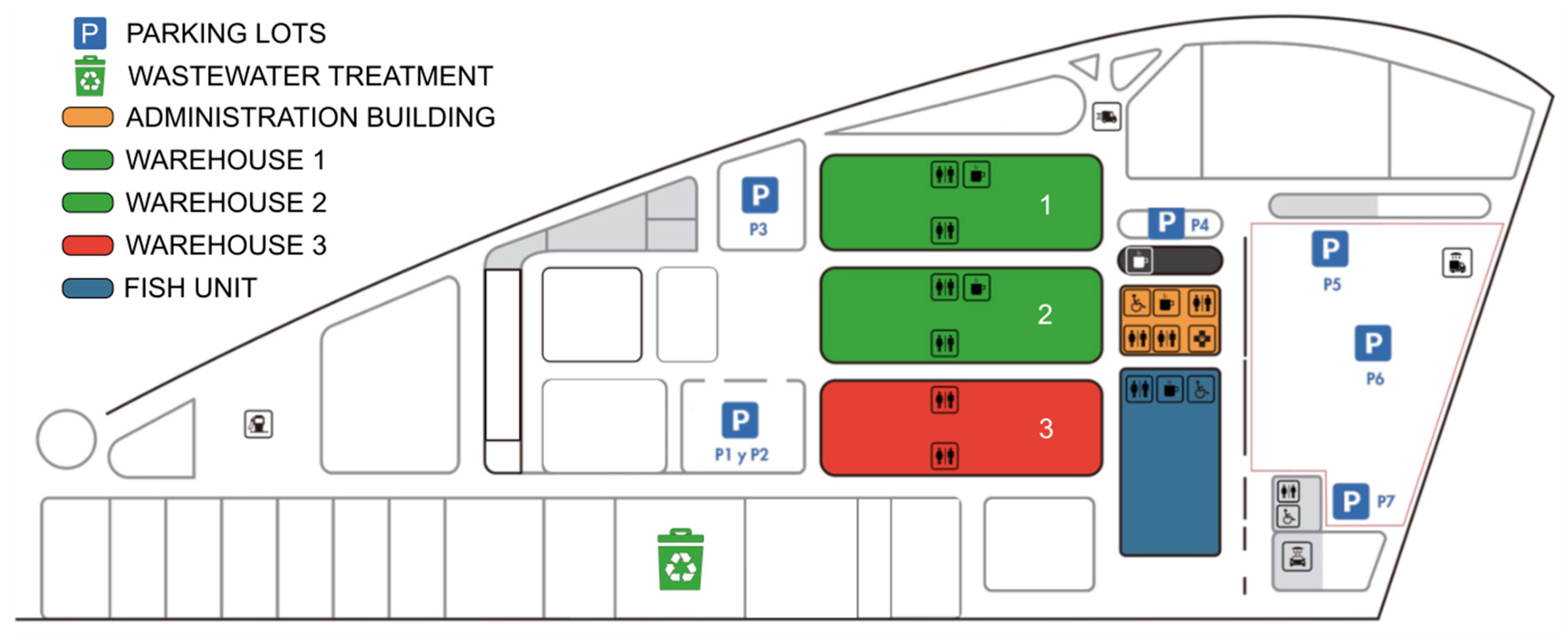
The logistics center adopted was a logistics and service center specializing in the food industry located in Spain. It provides services to other companies in the sector such as renting spaces equipped with proper refrigeration chambers if required, offices, 24/7 security services, parking lots, waste separation, and treatment, among others.
Figure 2 shows the plan of the whole site with the distribution of the available spaces. The specific units of interest for this study are highlighted and specified in the legend.
This study aimed to provide a more in-depth analysis into the energy and power consumption patterns of the main units of the logistics center and highlight some recommendations for improvement by reducing the costs associated with the electric energy consumed from the grid.
Among the units in
Figure 2, we emphasized the administration building; warehouses 1, 2, and 3; the fish processing unit; the waste treatment and pressure units; and the parking lots of the logistics center, which had an overall electricity consumption of about 650 MWh/year.
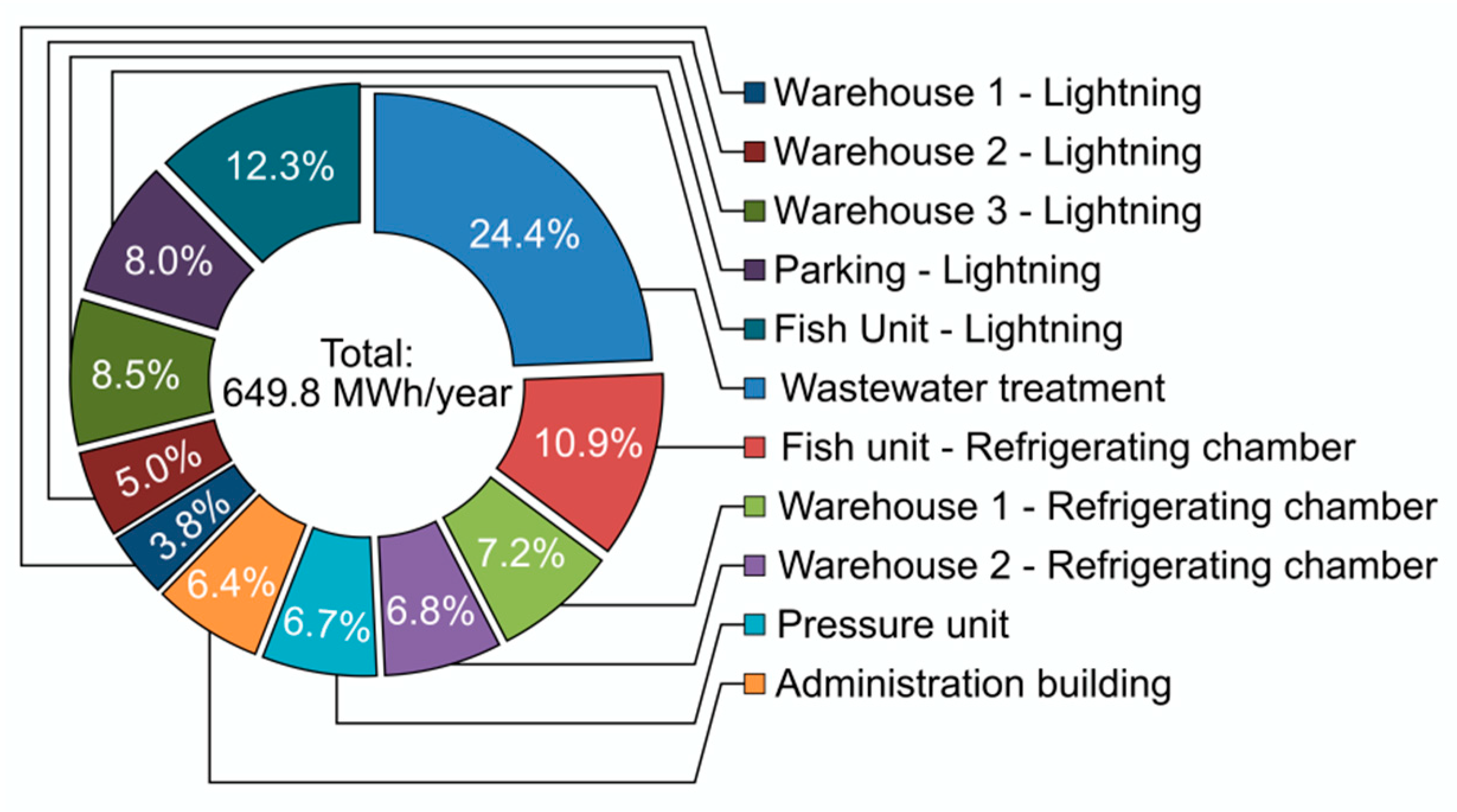
The share of the annual electric energy consumption required for the operation of each unit are provided
Figure 3, where 24.4% corresponded to the wastewater treatment, 24.9% to cooling in refrigeration chambers, and 37.7% to lighting the spaces.
The granularity of the dataset from the logistics center energy consumption (mainly its individualization by each of the main eleven units) allowed us to envisage the benefits of combining multiple loads into a single load, and verify the potential of improving the cost-effectiveness and the solar fraction for the different simulated PV sizing.
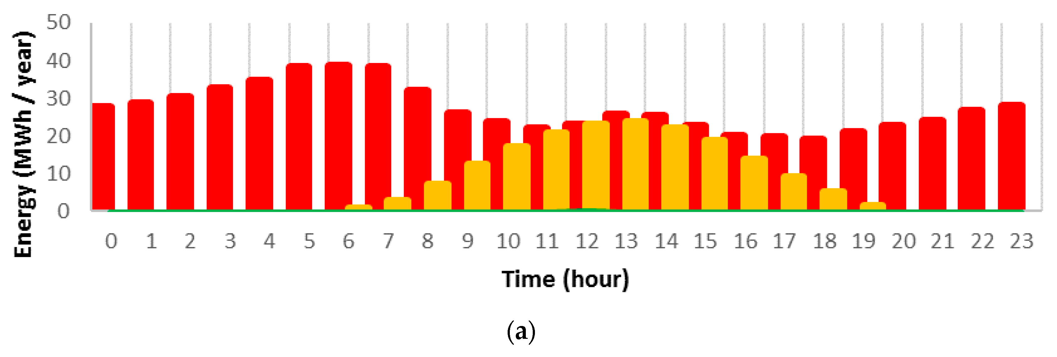
The average solar irradiation at the location of the logistics center is about 1.77 MWh/m2/year, which represents a potential of 188 kWh/m2/year of electrical energy using typical PV panels/inverters, with an average efficiency of 11% (considering typical efficiency rates of PV panels of around 13%, around 90% for inverters, and that the efficiency decreases over its lifetime).
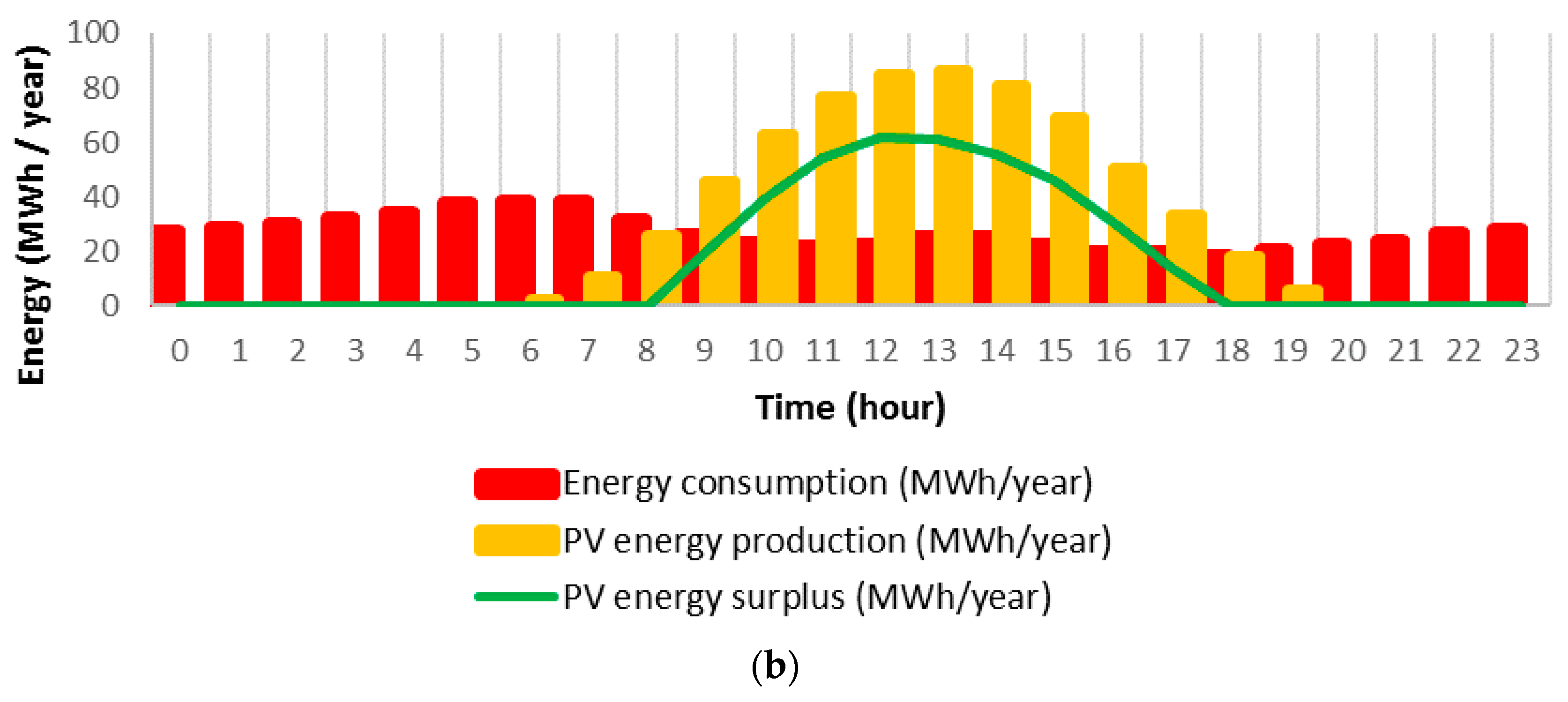
Figure 4a illustrates the summary of the hourly energy consumption (red), resulting in the annual consumption. The period of highest solar radiation, between 10 h and 16 h (yellow), represents 25% of the 650 MWh for the whole year. Preliminary calculations that do not consider the energy surplus (green) showed that PV panels distributed over an area of 911 m
2 could supply this amount of energy with a solar fraction around 27%, however, the detailed modeling and optimization revealed that these numbers could be further improved.
A hypothetical situation is shown in
Figure 4b that aims to clarify the need for detailed calculations where PV panels distributed over an area of 3340 m
2 would be able to supply the total annual energy consumption of the studied logistics center (650 MWh). This amount of energy would represent a solar fraction of around 40%, meaning that the 60% of energy surplus, produced between 9 h and 17 h (green), must have its allocation carefully planned.
This work included the study of the electricity consumption for eleven units of the logistics center (see
Figure 3). The electricity in these units is consumed mainly for two different purposes: lighting and the operation of specific equipment, namely the energy consumed by the refrigeration chambers, the wastewater treatment equipment, and the pressure unit equipment. The total demanded energy was considered initially to be obtained exclusively from the grid, and this situation constituted our base case.
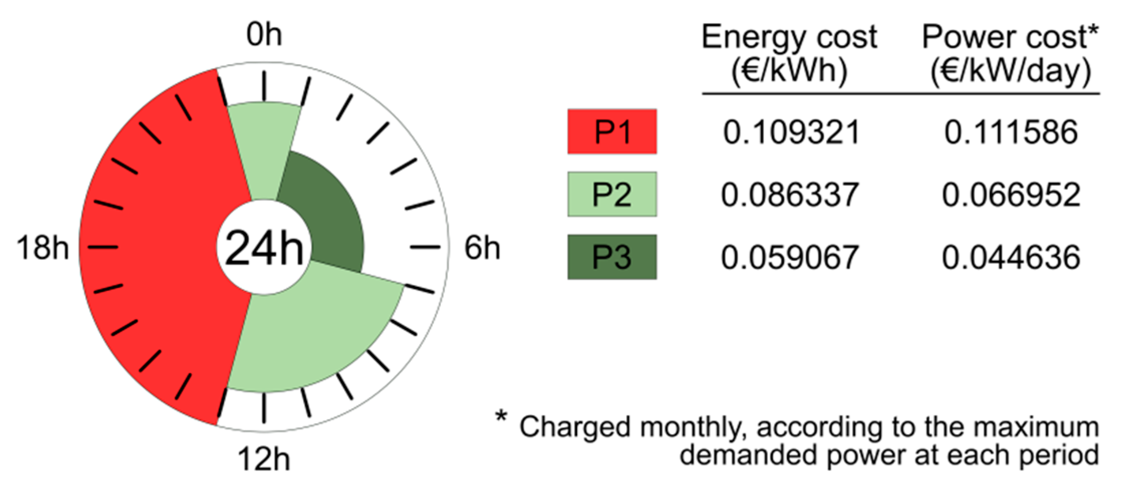
Every one of the eleven units had their own consumption pattern, and therefore, specifically contracted electricity and power. All contracts were made with Endesa S.A. for the “Tarifa Ahora” tariff of type 3.0A. This specific tariff is a low voltage tariff with three periods of charging (P1—peak period, P2—shoulder period, and P3—off-peak period). The electricity and power charge prices for these periods are shown in
Figure 5.
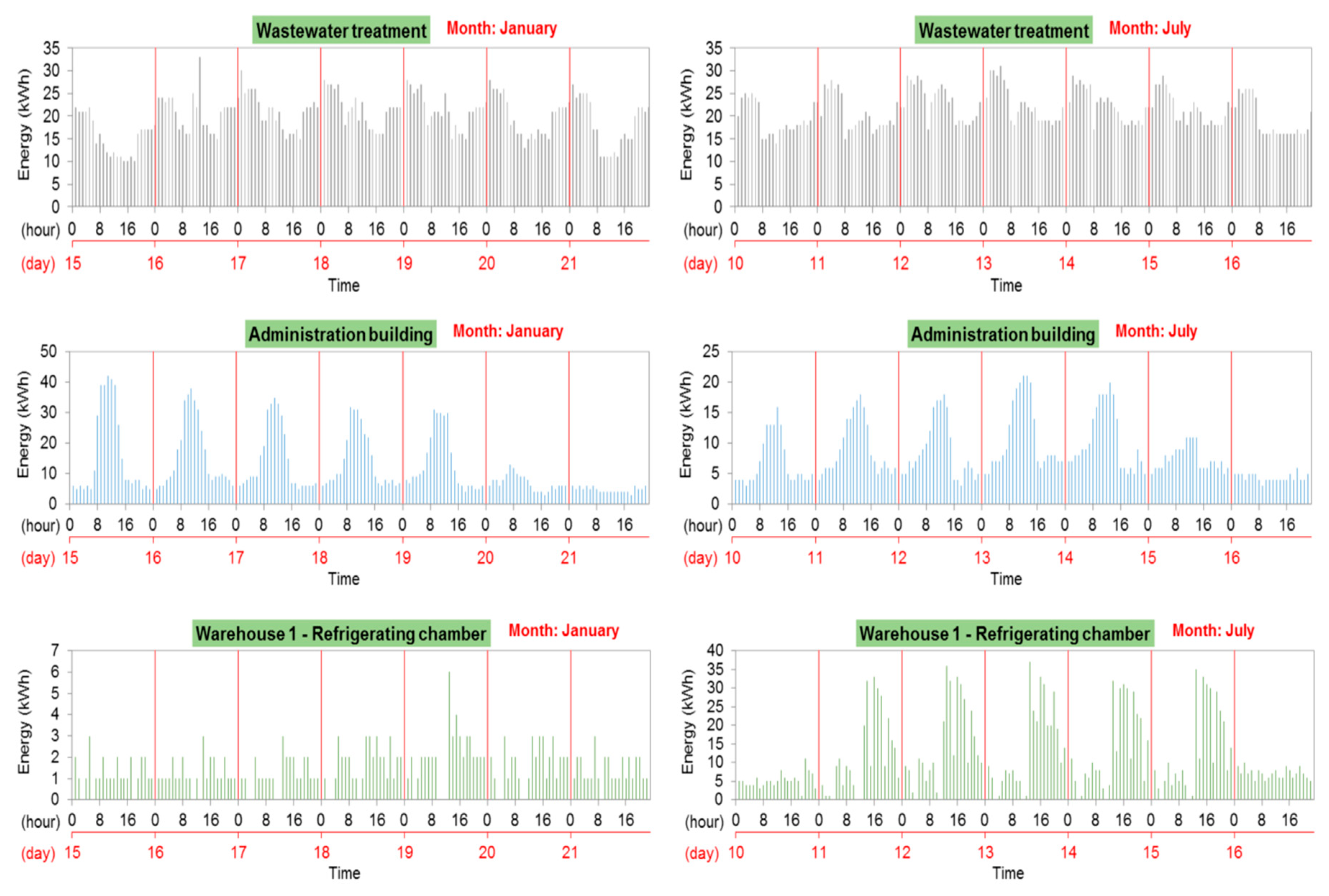
In
Figure 6, due to space limitation, we present the typical weekly consumption profiles of some of the units of interest for two different weeks during a natural year (one week in winter, and another in summer). These profiles were built for the 11 units within the scope to represent the seasonal effect on energy consumption.
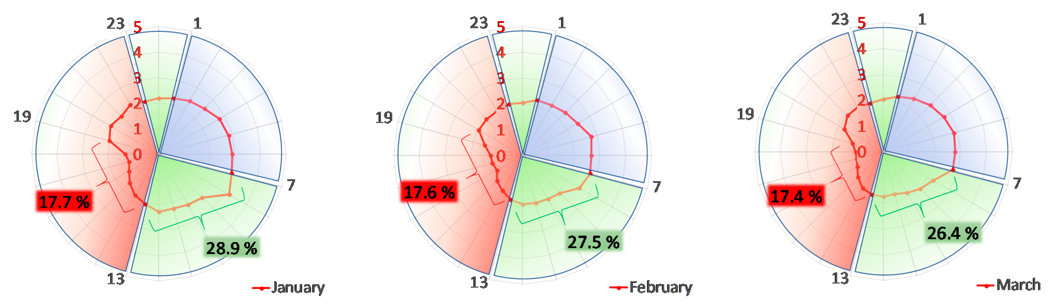
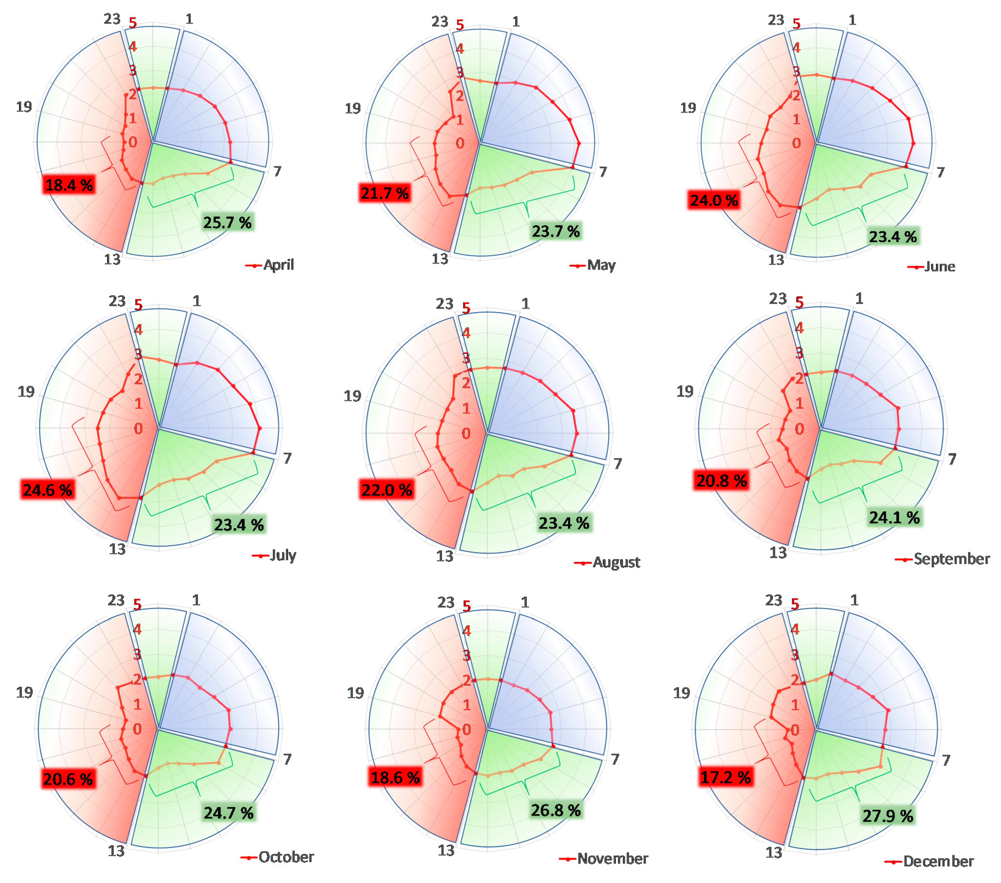
Figure 7 shows the monthly energy demand of the eleven units in MWh, and its distribution across the 24 h of the day. The summary of the twelve months represents the total amount of energy consumed annually, according to the energy demand input data, which was 650 MWh. The percentage amount of energy consumed before noon (07:00 to 12:59 h) and after noon (13:00 to 18:59 h) are also shown. Except for June and July, it can be verified that the energy consumption was predominantly during the period before noon. It is important to observe this aspect of the energy demand as it can influence the calculation of the optimal azimuth angle. If no energy exportation is considered, this characteristic would result in the optimal PV array azimuth angle not being directly to the south, but some degrees to the east, as there is more energy consumption during the period before noon.
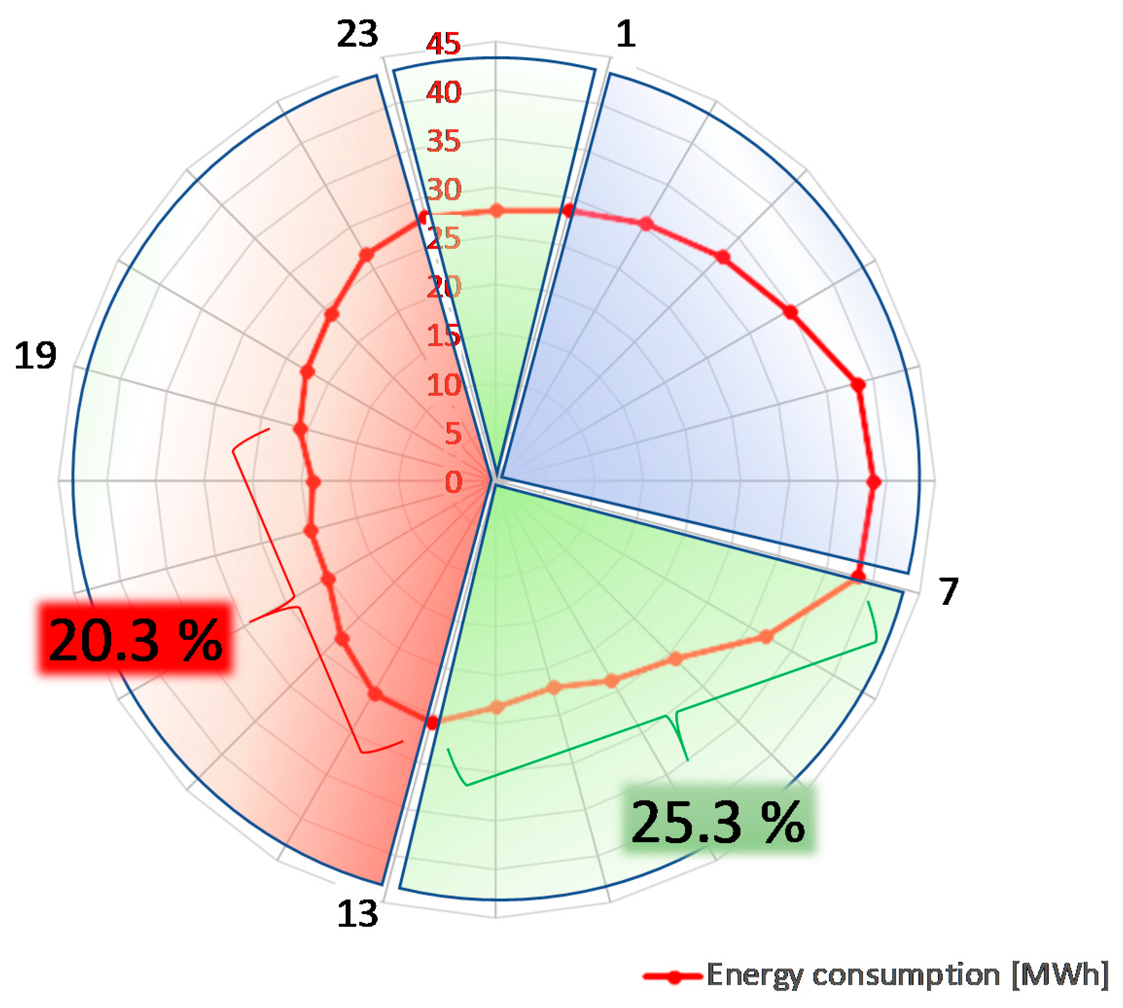
Figure 8 shows the annual energy profile and confirms that 25.3% of the energy was consumed during the period before noon and 20.3% after noon. Along the same line of the above-mentioned monthly analysis, if no energy exportation is considered, this characteristic would result in the optimal PV array azimuth angle not being directly to the south, but some degrees to the east.
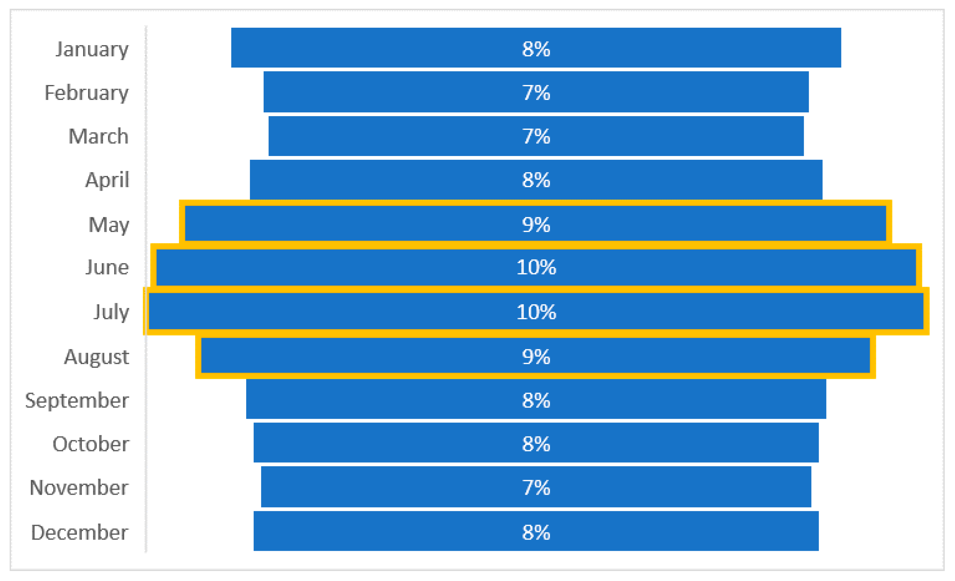
Another important aspect of the energy profile is shown in
Figure 9, where it was verified that around 30% of energy consumption is concentrated during the winter season. If no energy exportation is considered, and a fixed PV array slope angle is supposed to be adopted for the whole year, this characteristic would result in the optimal PV array slope angle being higher than the latitude angle in order to allow the PV array to be perpendicular in relation to the sun rays in winter. The coordinates of the Logistic Center location, Granada, are around 37°11′17.41″ N latitude and 3°36′24.01″ W longitude.
In the Results section, it is demonstrated that both the optimal azimuth and slope PV array angles will be different than those expected due to the influence of the energy export to the grid in a variable tariff scenario.
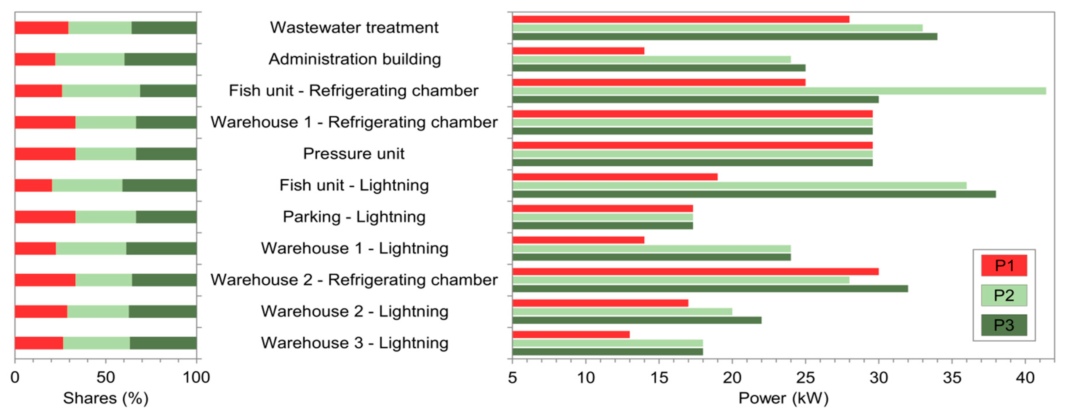
The initially contracted powers for each unit of the study (i.e., the base case contracts and the respective shares of P1, P2, and P3 are represented in
Figure 10).
2.2. Modeling and Simulations Steps
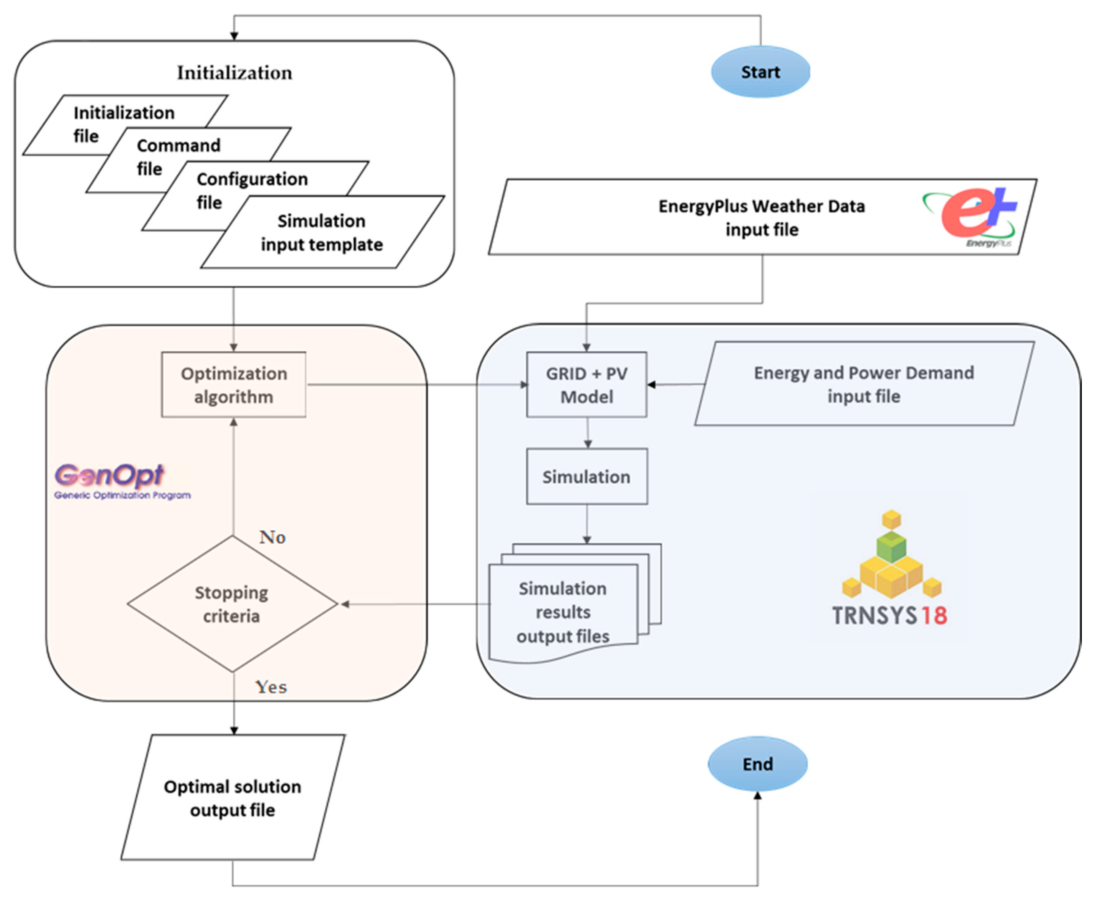
The modeling for the simulations was built using TRNSYS18 Simulation Studio [
16], and the metaheuristic algorithm based on particle swarm was performed by its optimization library component, the GenOpt Generic Optimization Program [
17]. The flowchart in
Figure 11 describes the main steps for the integration of these tools. In this study, the file information exchange was done manually, although some automation could be implemented using numeric calculation software (e.g., MATLAB), as detailed by Tulus et al. [
18].
For the modeling and simulation purposes, a life cycle time frame of 20 years was considered. The available annual consumption profiles, energy costs, and contracts were considered as “typical” and invariable from year to year during the whole period of the study (i.e., deterministic).
Three main steps can be made to achieve a reduction in the energetic expenses of the facility for a given consumption pattern. These are:
- (i)
Optimize the individual contracts of the units by adjusting their contracted powers;
- (ii)
Improve the energy efficiency by integrating the separate electricity contracts into one;
- (iii)
Reduce the dependence on the grid by incorporating alternative energy sources.
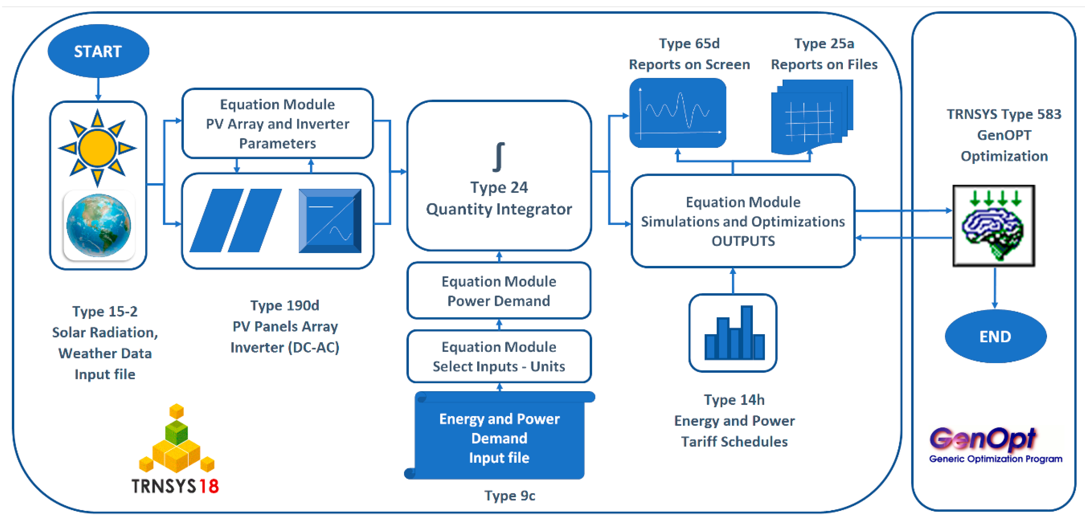
The main types (TRNSYS modules) used to build the model are described in
Figure 12 with their respective connections. Solar radiation and weather data from the location of the studied Logistic Center were obtained by Type 15–2 from an input file [
19] that supplies hourly information for an equation module, which is responsible for establishing the variables used for the calculations/simulations and the relationship with the main inputs and outputs of Type 190d, which reproduces the PV array and inverter (DC to AC).
The energy demand data file is read via Type 9c, and through an equation module, the separate units can be selected (or a combination of units) to compose the load configuration for the scenarios of the simulation and optimization. Additionally, the power demand details and calculations, are made in an equation module. All of the discrete data are integrated in a quantity integrator, Type 24, to compound the monthly and annual results.
A GenOpt plugin, Type 583, deals with the variables defined from the PV system and demand side modules in order to run the optimization algorithms with the aim of determining the minimal values of the objective functions, which is also described in the equation modules (e.g., LCC).
The initial consumption profiles were taken as parameters, which were been altered. The three options are quantitatively evaluated and discussed in the following sections. The quantitative evaluations were performed based on the mathematical equations described below, and aligned with the ASTM Standard Guide for Selecting Economic Methods for Evaluating Investments in Buildings and Building Systems [
20].
2.3. Mathematical Procedures
2.3.1. Life Cycle Costing (LCC)
The economic estimations in this work were undertaken based on the life cycle costing analysis method [
21]. This method includes all of the discounted expenses that originated during a specified time horizon of the facility’s operation, and has been used to analyze the feasibility of renewable energy solutions, as shown by Naves et al. [
22]. The total discounted expenses are defined below as the net present cost (NPC; depending on the case study, i.e. any of the considered actions described in
Section 2.5, this variable may refer to one single unit or to the combination of all units of the Logistics Center) of the project:
where
I0 (this variable may take the value of zero in the case that no investment is required) is the capital investment at the start of the project (Equation (2)). The investment capital (
I0) in this study is present only in Action 3 (see
Section 2.5.3) when photovoltaic panels have to be purchased.
I0 is defined as follows:
In Equation (2), nPV is the number of installed photovoltaic panels; PPV is the power supplied per panel in Wp/panel; and CPV is the PV price in €/Wp.
The
CFa is the annual net cash flow detailed in Equation (3); The annual net cash flow (
CFa), as defined in Equation (3), includes the annual costs of purchased energy (
CE) and power (
CP ) (depending on the case study, i.e., any of the considered actions described in
Section 2.5, these variables may refer to one single unit or to the combination of all units of the Logistics Center.) in Euro (Equations (5) and (6)), and the annual cost of maintenance (
CM) (this variable may take the value of zero in the case that no investment is required). The maintenance costs are considered only for Action 3 (see
Section 2.5.3).
The PWF (mentioned in Equation (1)) is the present worth factor, which reflects the time value of money. The PWF detailed in Equation (4) is the present worth of one Euro paid periodically in the future, where the nominal discount rate (d) and the time horizon of the analysis (N), in years, are considered.
The annual energy costs are obtained, as shown in Equation (5), where
E (also this variable may refer to one single unit or to the combination of all units of the Logistics Center) is the annually consumed energy in kWh and
CE is the energy price in €/kWh (see
Figure 5). Both
E and C
E vary depending on the index (
i), which represents one of the charging periods of the 3.0A tariff specified in
Figure 5.
The annual power costs are calculated in Equation (6). There,
D represents the cardinal number of days in a specific month
m;
Pch (also this variable may refer to one single unit or to the combination of all units of the Logistics Center) is the monthly charged power in kW; and
CP is the power price in €/kW/day. As in the previous equation,
Pch and
CP vary depending on the charging periods of the 3.0A tariff (
Figure 5) and the charged power may also vary from month to month.
A piecewise function in Equation (7) defines the charged power (Pch 3). This function is split in ranges depending on where the maximum demanded power of a specific month (Pdmax ) falls concerning the contracted power (Pc ).
2.3.2. Discounted Payback Period (PBP)
One conventional technique of the preliminary economic viability evaluation of a project is the payback period (PBP) [
23]. PBP is usually defined as the time required to recover the initial capital investment (
I0). In this particular work, the discounted payback period (
dPBP) was considered using Equation (8), where negative
I0 is the capital investment in the start of the project (Equation (2)) and
dSt is the discounted savings in period
t summed throughout the years between 1 and
dPBP.
The discounted savings (Equation (9)) can be obtained from the actualization of the annual savings of a particular project with an implemented action (see proposed actions in
Section 2.5). Those annual savings are the difference between the annual cash flows of the base case (i.e., current situation), and the cash flows of the proposed action. In Equation (9), the base case cash flows are referred to by the “*” symbol.
According to Equation (8), the dPBP for Actions 1 and 2 will be zero, since no investment costs are required for their implementation.
2.4. Optimization Models
Model M-1 (Equation (10)) was used to obtain the minimum
NPC of every unit of the logistics center for Action 1 (see details in
Section 2.5.1). This model minimizes the
NPC of a logistics center unit, subject to Equations (3)–(7), by varying the contracted powers (
Pc) (one for each charging period of the 3.0A tariff) between the specified lower (
PcL) and upper (
PcU) bounds. Later, the minimum NPCs are added up to represent the total net present cost of the project over the analyzed timeframe.
Additionally, model M-1 was used in Action 2 (see details in
Section 2.5.2), where the minimized
NPC does not represent the values of the separated units, but the combined cost of all eleven units studied in this project, considered as a single load from an electrical point of view. Equations (2)–(6) and the lower (
PcL) and upper (
PcU) bounds were conveniently modified to correspond to the combination of the units.
Due to the nonlinearities of the model M-1, it was solved using the TRNSYS18 Simulation Studio [
16] and its optimization library component, the GenOpt Generic Optimization Program [
17] in a single-objective optimization (SOO) process based on the NPC with a LCC perspective. This approach can be found in similar studies using multi-objective optimization (MOO) processes as performed by Li et al. [
24] and Asadi et al. [
25].
Finally, model M-2 (Equation (11)) was implemented for Action 3 (see details in
Section 2.5.3), where
NPC is minimized subject to Equations (2)–(7) and additional energy balances provided by the simulation software. The decision variable in model M-2 is the number of PV panels, which were installed in strings of seven individual panels connected in series. This distribution is advisable for security purposes and to adequate the DC voltage to the input range of market inverters (e.g., the Solar Inverters List published by NATA, National Association of Testing Authorities [
26]).
Due to the strong nonlinearities of the optimization model M-2, which additionally contains implicit equations evaluated by the simulation software, the model can be solved using a metaheuristic algorithm based on particle swarm implemented in the optimization tool, GenOpt (see
Figure 11).
2.5. Scenarios
As mentioned in the previous section, we developed three different scenarios, and three possible actions whose implementation is to be evaluated by the decision-makers. These actions are detailed below and, for the sake of comparing the results between them and the current situation, a base case was introduced as the current operation state of the Logistics Center in
Section 2.1.
2.5.1. Action 1: Optimization of Individual Contracts
This action, in theory, would not require additional expenses for the company. The only required action would imply the revision of each of the current contracts, according to the optimization results provided in
Section 2.1.
2.5.2. Action 2: Optimization of Combined Contracts
In Action 2, we suggest considering the possibility of a combination of the eleven separate electricity contracts into one contract.
2.5.3. Action 3: Integration of Photovoltaic Panels (PV)
The integration of renewable energy sources can suppose a significant profit, but in contrast to the previous two actions, an initial investment is required. However, over time, the savings can potentially be more significant and, on top of that, it can have multiple environmental benefits.
Action 3 would imply the integration of PVs to reduce the dependence on the grid. In this case study, the energy demand of the separate units was considered as one combined demand (as in Action 2), which would be partially covered by the PV panels (the grid will provide the rest). The exportation to the grid of the energy excess produced by the PVs (surplus) is discussed considering the most common FiT (feed-in tariff) approaches, named as net metering and net billing [
27].
As the solar energy sector evolves rapidly, the efficiency, performance, and costs of PV technology regularly changes, that can be verified in a variety of reports such as those published by the International Renewable Energy Agency (IRENA) [
28] and the Fraunhofer-Institute for Solar Energy Systems (ISE) [
29]. For that reason, we considered three scenarios based on parametric costs (€/Wp) issued by the National Renewable Energy Laboratory (NREL) [
30], reflecting the aspect of the price of the PV panels, cPV, (which includes the module itself, the structure, and the installation costs):
Scenario A—low cost, represents 0.68 €/Wp;
Scenario B—intermediate cost, represents 1.18 €/Wp; and
Scenario C—high cost, represents 1.48 €/Wp.
The maintenance costs (cM) in each of the three scenarios were 0.02 €/Wp/year.
2.5.4. Exportation of PV Energy Surplus to the Grid
If we consider the net metering configuration where the exported energy compensates the energy consumption, the simulations aimed to verify the PV system’s optimal sizing by focusing on the potential cost reductions. As the balance of calculating the monthly energy bill on this configuration occurs in terms of energy, the price of exported energy can be considered as the retail price, that is, the same price as the consumed energy from the grid.
In the net billing configuration, the price of the exported energy tends to be close to the wholesale price. In order to analyze the feasibility of this configuration, simulations with three different values of exported energy were adopted, based on the retail price, of 30%, 60%, and 90% of the retail price.
At both configurations, the limit of PV exported energy in the simulations was set to the amount of energy effectively consumed in the same month in order to avoid unfeasible results.
In order to obtain more accurate results related to the exportation benefits, the exportation tariffs adopted in the simulations (
Table 1) were calculated from the weighted average of the annual exported energy. Weights of 57.39% and 42.61% were obtained from the simulation results analysis, which allowed us to verify the annual average amount of energy exported during the periods P2 (07:00 h to 13:00 h) and P1 (13:00 h to 23:00 h), respectively. For the optimization process, the objective function was to minimize the LCC.
2.6. Assumptions
Below is presented the set of additional assumptions and simplifications considered in this work, but not mentioned earlier.
The adopted electricity tariffs were based on the 2017 electricity bills of the Endesa “Tarifa Ahora” type 3.0A (see
Figure 5). The available consumption profiles were considered to be representative for the whole period of study. For the net present cost (
NPC) calculations, we adopted an annual discount rate of 2% in order to compensate increments on the energy prices. The time horizon of the analysis (
N) was 20 years (expected lifetime of the PV system). The simulation model included the hourly based climatic data of Granada (Spain) obtained from EnergyPlus Weather Data [
19] and a data file covering a natural year of energy consumption and power demand (8760 h).
According to a publication by the NREL (National Renewable Energy Laboratory) [
31], the output power of polycrystalline silicon PV panels drops on average 0.5% per year. This means that in a timeframe of 20 years, the power output of a PV panel will decrease 9% and if we considered a rated efficiency of 14.7% [
32], there is an efficiency drop of 1.3%. These numbers are based on previous work such as those performed by Kitamura et al. [
33]. However, the lack of historical data related to the most recently manufactured PV panels (with improved efficiency rates) and doubts about the non-linearity of the lifespan efficiency degradation rate, led the authors to avoid including this factor in the calculations and adopted an average PV/inverter efficiency value over the lifetime.
The average efficiency of the PV panels for this case study was 11.7% with a module efficiency of 13.4% and inverter efficiency of 91.5%. Each single-panel occupies a surface of 1.64 m
2 and must be connected in parallel sets of seven panels each (the separate sets are connected in series). The complete list of the PV specifications and the main electrical specifications used to configure the PV component (type 190) on the TRNSYS model, according to the calculation method presented by DeSoto et al. [
34], can be found on the manufacturer’s website [
35].
For the simulations and optimizations, the PV array slope and azimuth angles were initially considered as 0 degrees, which means that the PV panels were in a horizontal position and faced directly to the south. Due to the characteristics of the case study, no shading simulation effects were considered in this study.
3. Results
3.1. Results Considering No PV Surplus Energy Exportation
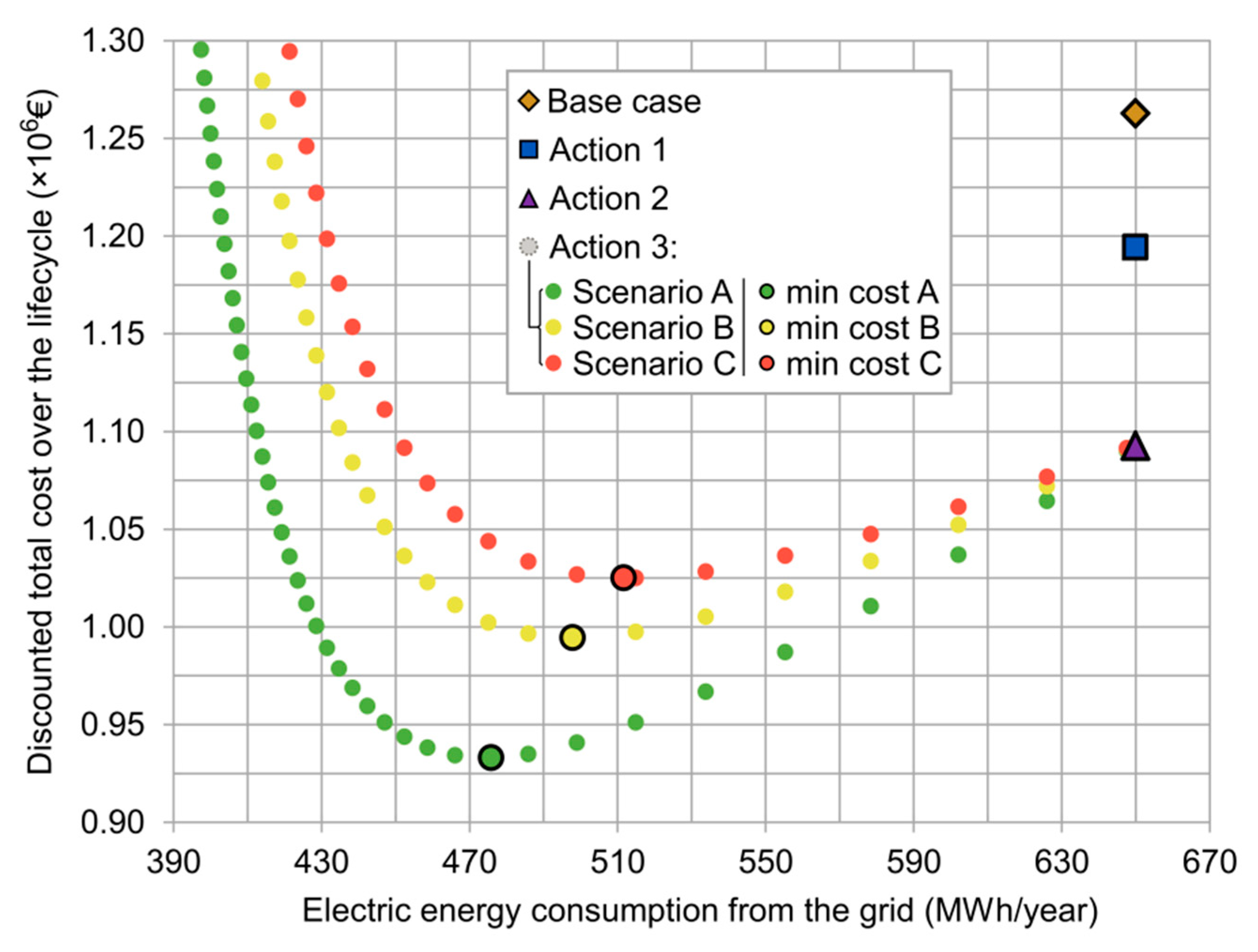
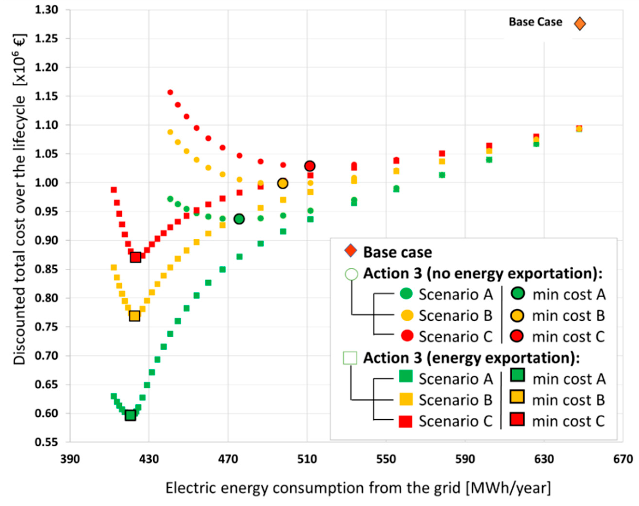
Figure 13 presents the summarized results of the three proposed actions of this study and the current state (base case) in terms of the (total) net present cost and amount of electricity consumption.
While Action 1 and Action 2 do not require essential equipment investment, consisting mainly of reviewing the contracts and the connection configuration between the loads and the grid (electrical company issues), Action 3 requires special attention to avoid oversizing the PV.
Additionally, in
Figure 13, the adverse effect on the LCC due to the oversizing of the PV panels in Action 3 can be verified if we move from the right to the left side on the plotted points of scenarios A, B, and C.
The right side of the highlighted optimal points A, B, and C represents the region where the increase in PV panels corresponds to a LCC reduction. The left side represents the region of oversizing, where an increase in the PV panels increases the total costs, meaning that it is unfeasible from an LCC perspective, unless an appropriate use for the surplus energy is addressed, as commented above (see
Section 1).
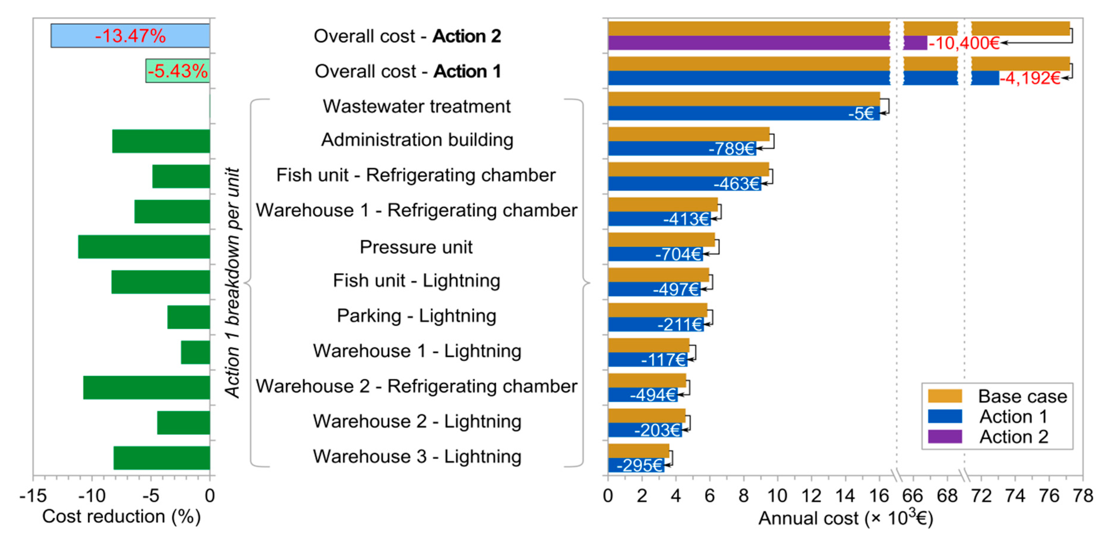
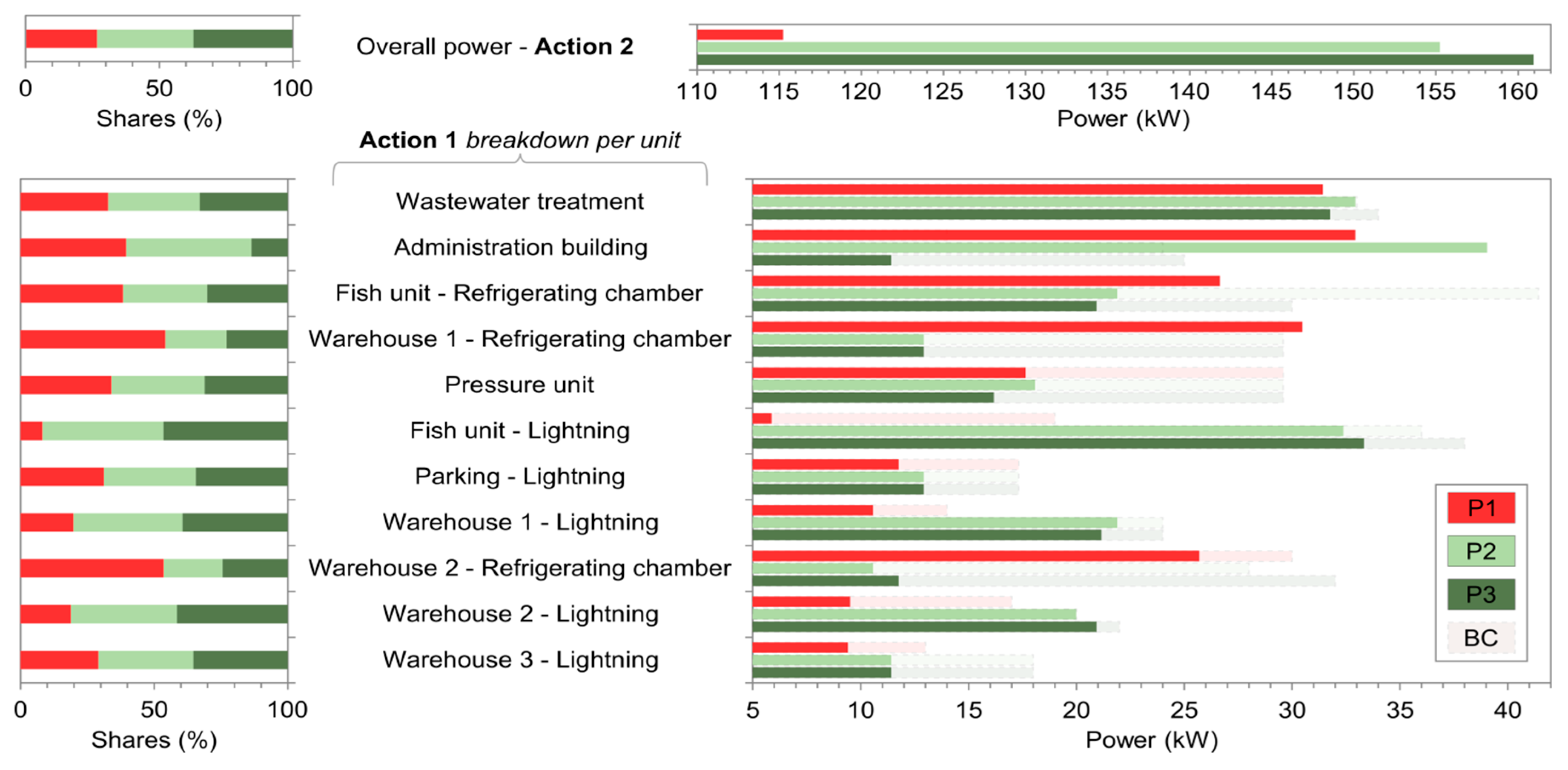
Action 1 represents 5.43% of cost reductions after revising the contracted powers for each separate unit of the study. In the same direction, Action 2, maintaining the same energy consumption from the grid as Action 1 and the base case, achieved a reduction of up to 13.47% in costs (compared to the base case). Recall that Action 2 would imply the combination of the demands of all units into one combined demand. A more detailed annual cost (i.e., annual cash flows) breakdown of Actions 1 and 2 can be found in
Figure 14, and the changes to be implemented are shown in
Figure 15.
Action 3, and more specifically, its optimal scenario A (see
Figure 13), can present as much as a 26.13% cost reduction when compared to the base case. This solution would also contribute to 26.8% in the reduction of grid dependency. The other scenarios and their optimal and suboptimal solutions can also potentially provide cost reductions over the lifecycle of the study.
3.2. Results Considering PV Surplus Energy Exportation to the Grid
Figure 16 illustrates the comparisons of the simulations considering the exportation of the PV energy surplus with those results obtained in the scenario of Action 3. The energy consumption from the grid and the LCC decreased with the installation of more PV panels, and the optimal values of the LCC were obtained before the energy consumption from the grid reached the limits of the maximum solar fraction (around 35%). Additional investments can bring about significant reductions in the LCC with payback periods similar to the scenarios where no energy surplus was exported to the grid.
When considering the energy exportation to the grid, supposing the net metering configuration (exported energy price considered as 100% of the retail price), the optimal number of PV panels to be installed for each scenario would increase from 630 to 1617, from 497 to 1533, and from 434 to 1512, respectively. The exportation of energy allows the LCC savings to move from 21% to 39% in the intermediate configuration, Scenario B.
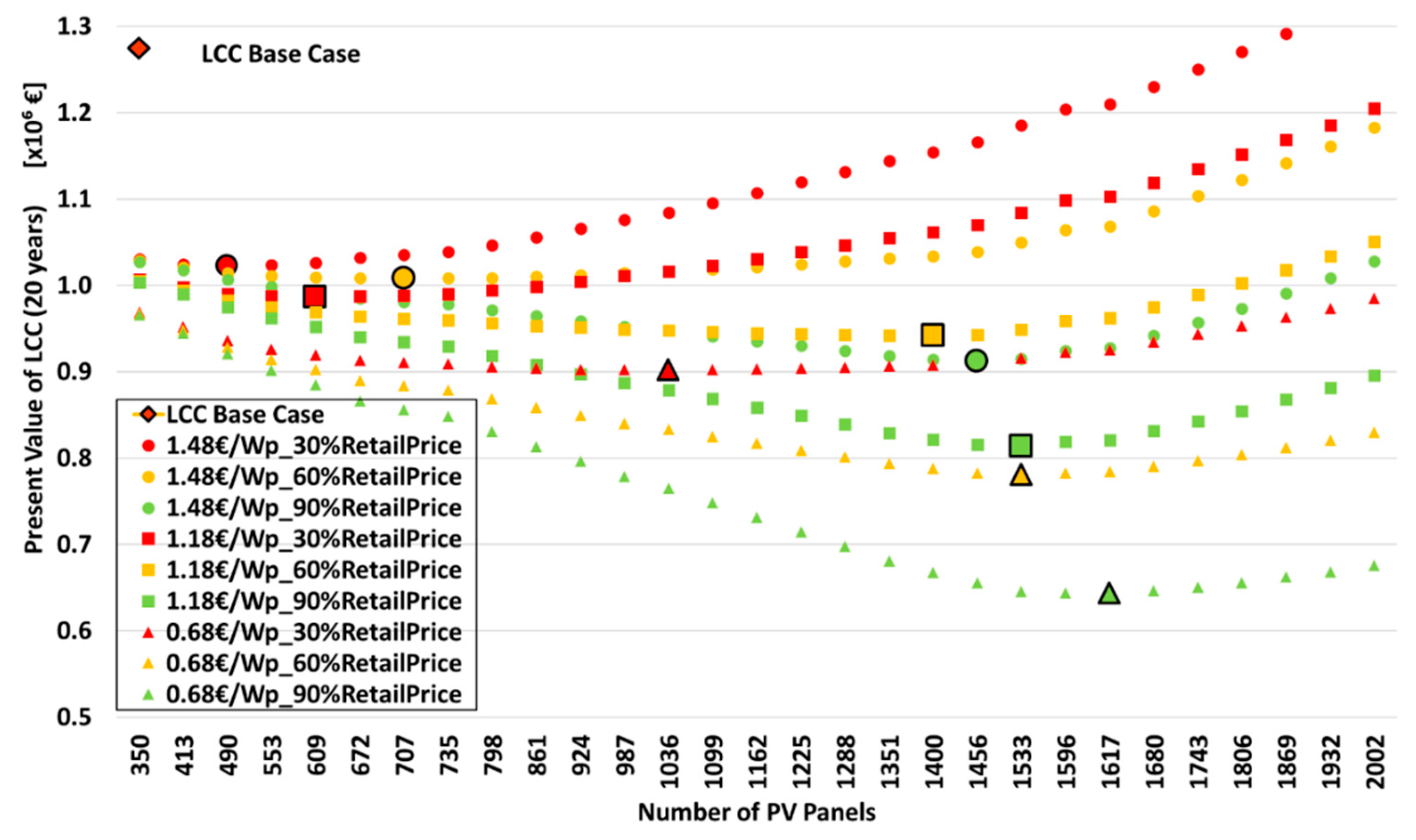
In addition, based on Action 3, and considering the energy exportation to the grid, in a net billing configuration, the optimal number of PV panels that would produce the lowest LCC values are shown in
Figure 17.
In order to verify the influence of the exported energy price, for each of the three scenarios mentioned before based on the prices of the different PV panels (0.68, 1.18, and 1.48 €/Wp), three values were adopted in the simulations, that is, 30%, 60%, and 90% of the retail price of the energy, representing three hypothetical wholesale prices.
3.3. Effect of the PV Array Slope and Azimuth Angle on the Results Considering No PV Surplus Energy Exportation to the Grid and PV Energy Surplus Exportation
The results presented above considered the PV array slope and azimuth angle as 0 degrees. In order to verify the influence of these factors on the results, the simulations and optimizations were performed with the aim to reach the optimal slope and azimuth angles and to measure their effect on the LCC obtained with the initial conditions. For the simulations, we considered fixed angles of the PV array during the whole year, and no tracking systems were considered.
Scenario A (Action 3) was used as the reference. When considering no PV surplus energy exportation, the optimization reached an optimal slope angle of 19.5 degrees and an optimal azimuth angle of −2.5 degrees, representing a LCC saving of 0.83% (from 936,569 to 925,959 Euros), mainly due to the slope angle optimization.
When considering the PV surplus energy exportation, the optimization reached an optimal slope angle of 35.5 degrees and an optimal azimuth angle of 3.0 degrees, representing a LCC saving of 9.00% (from 596,146 to 481,449 Euros), 8.99% due to the slope angle optimization, and 0.01% due to the azimuth angle optimization.
Although the installation of the PV array with angles higher than 0 degrees could represent additional costs with the support structure, these results show that this option is feasible, if considering the PV surplus energy exportation to the grid.
4. Discussion
As shown in
Section 3, when not considering the PV energy surplus exportation, an oversizing of the PV field would increase the total costs significantly, while the reduction in grid energy consumption is marginal.
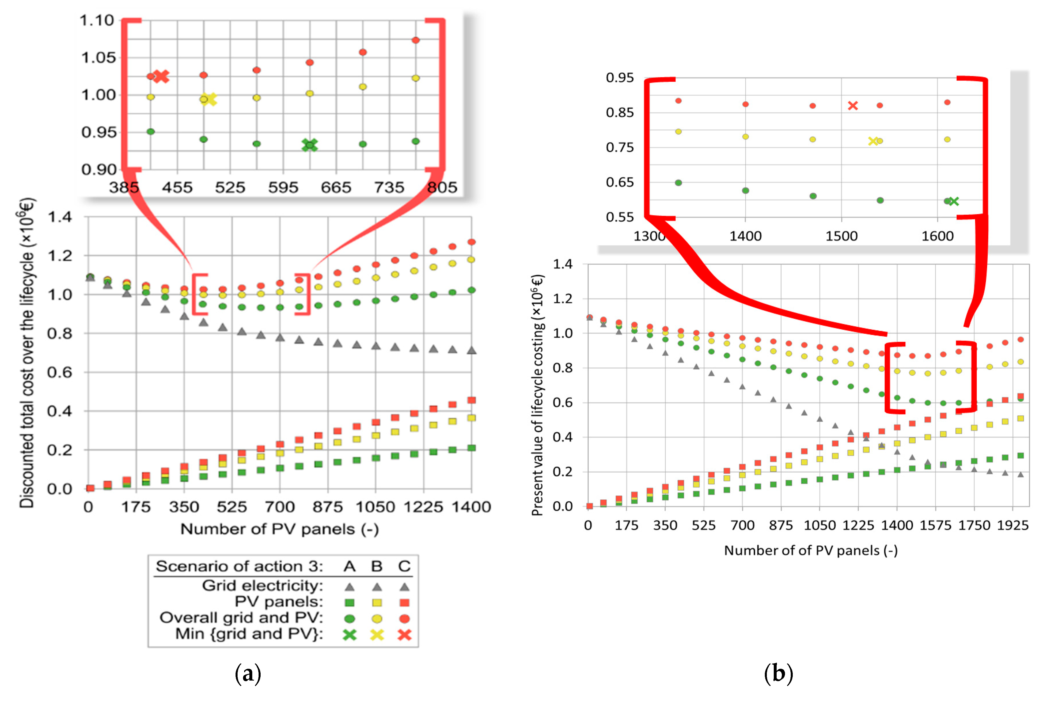
However, the possibility of exporting surplus energy to the grid allows for more flexibility in the energy and cost management. Despite the solar fraction, which limits the amount of PV energy used to attend the demand, the possibility of exporting the surplus energy makes it feasible to implement more PV panels, representing a significant reduction in the LCC, as verified by comparing
Figure 18a,b.
The cost breakdown of Action 3 and scenarios A, B, and C for both configurations (PV energy exportation considering a net metering approach, and no energy exportation) is shown in
Figure 18a,b, as a function of the number of PV panels. The colored square points correspond to the investment cost of PVs, the grey triangle points are the electricity costs billed by the electricity provider (Endesa in this case), and the colored circle points show the overall LCC (i.e., the summation of the PV investment, the charged grid electricity and the compensation of PV energy exportation).
The zoomed areas indicate the optimum solutions for scenarios A, B, and C. The optimal number of PV panels to be installed for each scenario was 630, 497, and 434, if no PV energy exportation was considered, or 1617, 1533, and 1512 when exporting the PV energy surplus, respectively.
Making a rough approximation of the area that would be occupied by these panels, we obtained 1040 m
2, 820 m
2, and 716 m
2 for every optimal solution of scenarios A, B, and C if no PV energy exportation is considered, or 2668 m
2, 2530 m
2, and 2495 m
2, considering the possibility of PV energy surplus exportation, respectively. Action 3 would require an initial investment, which will strongly depend on the assumptions described in
Section 2.6.
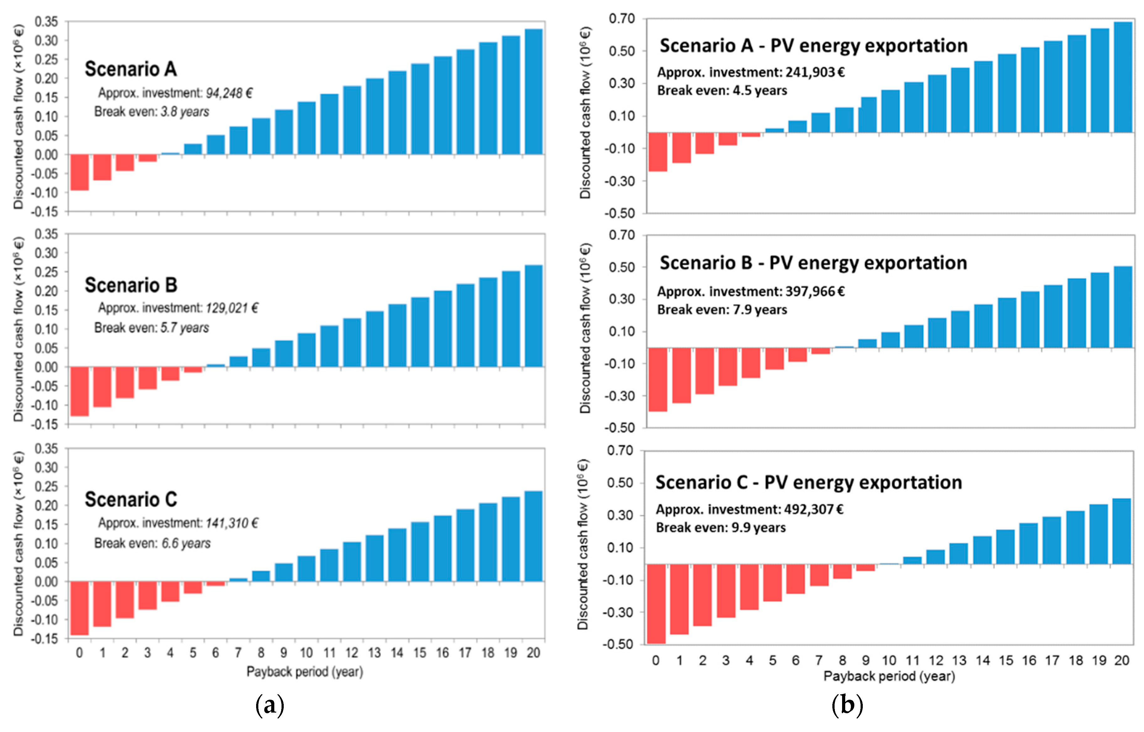
Figure 19 presents the effects of the PV energy surplus exportation to the grid on the investment costs and payback periods. In Scenario A, for example, it can be verified that despite the increase in the investments due to the PV system sizing (from 630 to 1617 panels), the payback period increases to less than one year and the LCC savings go from 26.5% to 53.2%.
The above-mentioned scenarios are feasible to implement since the entire rooftop available area of the industrial units was around 24,200 m2 (three units with 5000 m2 each; three units with 3740 m2, 2040 m2, and 1830 m2 respectively; one commercial unit with 570 m2; one administration unit with 940 m2). The parking area corresponded to 25,830 m2, representing an option to implement PV panel coverages (canopy).
Depending on the cost of the PV panels, the investment cost and break-even point will vary significantly, so precautions must be taken while defining the PV costs above-mentioned.
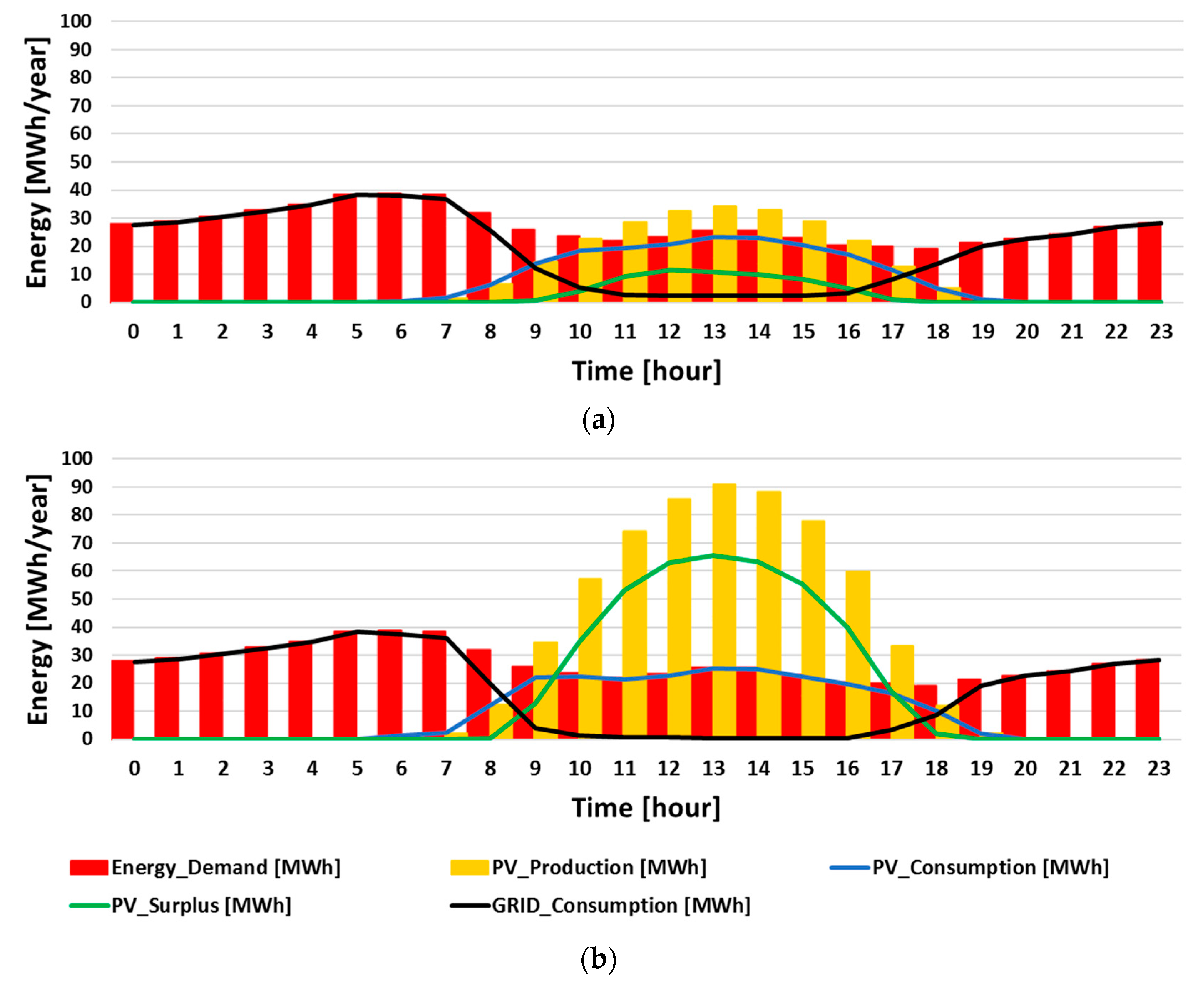
Figure 20a,b show the energy profiles including the energy demand, the PV production, and consumption from the grid and from the PV system, and the PV surplus energy for both options, with no PV surplus exportation and with PV exportation to the grid. Scenario A (Action 3) and the net metering configuration were taken as the reference for these graphics.
Figure 20a reproduces the optimal values obtained using LCC as the objective function, and it was possible to verify that some surplus energy was obtained (60 MWh/year) due to the characteristics of the energy demand and the PV energy production. This scenario represents LCC savings of 27.33%.
Figure 20b reproduces the option of PV surplus energy exportation and the posited results are more tangible. It can be verified that the energy consumption from the grid was close to zero between 10:00 h and 16:00 h. Practically all the total PV energy surplus was exported (407 MWh/year) and allowed for LCC savings of 62.22%. This option shows that the PV energy surplus exportation can be considered as a way to store the exceeding energy in the grid and use it when necessary. Despite political factors having significant influence on these results, the feasibility of this solution seems to be attractive from an economic point of view.
5. Conclusions
The three actions proposed in this study (Action 1: Optimization of individual contracts; Action 2: Optimization of combined contracts; Action 3: Integration of photovoltaic panels, with three different PV price scenarios) could potentially contribute to savings of different important subjects to the described simplifications and assumptions. Further investigations in any of these directions would be required to provide more detailed results and indications.
However, a 5.43% cost reduction could be achieved by the implementation of slight changes to the contracted power for each separate contract. A higher cost reduction of up to 13.47% could be reached in the case of unifying the contracts. In the previous two cases, no significant additional investment costs would be required.
If significant investments are taken in a life cycle perspective (LCC), their feasibility can be unveiled. To attain higher cost reductions in the long-term (up to 21% in the intermediate configuration, Action 3, Scenario B) and at the same time reduce the consumption of electricity from the grid to around a quarter, an investment of 129,000 € would be needed, which is expected to pay-off in less than six years. Simulations and optimizations showed that the energy exportation to the grid could increase the LCC savings in this scenario of up to 39%, and reduce the energy consumption by up to 35% (limits of solar fraction obtained in this location). Although the necessary investment in this configuration would increase to 398,000 €, the payback period is less than eight years.
Any other lower improvements can hypothetically be achieved with fewer investment costs and smaller payback periods.

 ,
, 


