Is Deployment of Charging Station the Barrier to Electric Vehicle Fleet Development in EU Urban Areas? An Analytical Assessment Model for Large-Scale Municipality-Level EV Charging Infrastructures

Abstract

This work investigates minimum charging infrastructure size and cost for two typical EU urban areas and given passenger car electric vehicle (EV) fleets. Published forecasts sources were analyzed and compared with actual EU renewal fleet rate, deriving realistic EV growth figures. An analytical model, accounting for battery electric vehicle-plug-in hybrid electric vehicle (BEV-PHEV) fleets and publicly accessible and private residential charging stations (CS) were developed, with a novel data sorting method and EV fleet forecasts. Through a discrete-time Markov chain, the average daily distribution of charging events and related energy demand were estimated. The model was applied to simulated Florence and Bruxelles scenarios between 2020 and 2030, with a 1-year timestep resolution and a multiple scenario approach. EV fleet at 2030 ranged from 2.3% to 17.8% of total fleet for Florence, 4.6% to 16.5% for Bruxelles. Up to 2053 CS could be deployed in Florence and 5537 CS in Bruxelles, at estimated costs of ~8.3 and 21.4 M€ respectively. Maximum energy demand of 130 and 400 MWh was calculated for Florence and Bruxelles (10.3 MW and 31.7 MW respectively). The analysis shows some policy implications, especially as regards the distribution of fast vs. slow/medium CS, and the associated costs. The critical barrier for CS development in the two urban areas is thus likely to become the time needed to install CS in the urban context, rather than the related additional electric power and costs.

1. Introduction

Mitigating the effects of climate change through greenhouse gas (GHG) emissions reductions is one of the key challenges of the 21st century. At the core is the issue of overall energy consumption as well as the need for stronger decarbonization policies. Within this picture, transport sector plays a big role, globally and at European level: EEA data shows that in 2016, it accounted for a 33.2% share of EU-28 final energy consumptions and for a 24.3% share of GHG emissions [1]. Road transport accounted for 72% of GHG emissions and, within that sector, cars accounted for 60.7%. Moreover, half of EU-28 NO_x emissions and at least 15% of PM10, PM2.5, SO_x and CO emissions are transport-related [1,2]; finally, European transport energy needs are fulfilled by fossil fuels use for more than a 94% share [1].

Several alternative energy sources and renewable fuels are available—with different level of technology readiness and market penetration—in order to reduce dependence on fossil fuels: among them we find biofuels such as biodiesel and bioethanol, renewable hydrocarbons, ligno-cellulosic ethanol, biomethane, renewable fuels of non-biological origin (RFNBO) recycled carbon fuels, renewable e-fuels, renewable hydrogen, electricity, etc. None of these alternative fuels and sources alone will ever completely substitute fossil fuels, at least in a short term, and most of the forecasts see them coexisting in future fuel mixes [3]; in 2016, in EU-28, biofuels accounted for the bigger share, covering 4.6% of total final fuel consumption [1].

Anyway, rapid cost reduction of solar and wind power technologies created strong prospects for further electrification of end-use sectors. Within this framework, electric vehicles (EVs)—especially passenger cars—are one of the most pursued solutions to achieve large-scale transport sector decarbonization; anyway, they are not a “drop-in” solution, since they need a new and alternative charging infrastructure. Official documents such as the Alternative Fuels Infrastructure (AFI) Directive [4] and the National Plans for alternative fuels and EV charging infrastructure such as [5,6] are of interest because they express governments forecasts about future EV fleet size and formal recommendations on topics such as the minimum number of charging stations (CS) to be deployed and the minimum EV/CS expected ratio.

It is expected that urban areas will be the place of a large-scale infrastructure deployment in short to mid-term, since they are the most suitable for actual EV use and would receive maximum benefit from noise and local polluting emission reductions that are related with the shift from internal combustion engine vehicles (ICEV) to EV. To this regards, stakeholders and decision makers could benefit from reliable predictions on the dimension and cost of a charging infrastructure suitable for, i.e., a municipality area.

Literature already presents several studies on EV charging infrastructures, which analyze the topic from a multitude of points of view. Many of them evaluate the optimal positioning of a given set of CS through geographic information system (GIS) procedures, such as [7,8] or through traffic flows analysis such as [9]; they develop a model taking into account residential statistics, parking area information, electric power distribution network position and other data to define the optimal position for charging stations, but usually the input data about the number of CS to be deployed have little or no connection with data on EV fleets circulating in the area or on forecasts about that. Other studies focus on business and profitability analysis of a specific CS installation [10], while other analyze the possible interactions between charging EV and RES electrical generation that could take place in urban areas, such as the one from PV installations [11,12].

Finally, several papers analyze the topic of optimal sizing of EV charging infrastructures. Unfortunately, reports that specifically evaluate cost and size of large-scale deployments, using real data and forecasts (such as [13,14]) usually refer to national or international levels and give as output highly aggregated information; this makes it difficult, afterwards, to scale them down to a more local level. Several studies can be found, that address the problem at a regional and municipality level: [15] analyzes the German region of Stuttgart, but it focuses its model on CS availability rate and is not applied to a real scenario. The study [16] is related to the Italian province of Florence and uses GPS real data from around 12,000 ICE vehicles, extracting driving and parking patterns to size the charging infrastructure; anyway, it does not explicitly give as an output a number of CS and the relative cost, and it does not consider a temporal evolution of the analyzed situation. Lastly, [17,18] give as an output the forecast size of the charging infrastructure for two different Swiss municipalities, but neither of them give a proper explanation on the methodology used.

Scope of this work is to define the optimal size of a minimum cost charging infrastructure, suitable for deployment in an urban area and able to cope with the requests of a given passenger car EV fleet. This study focuses only on EV passenger cars since they account for the vast majority of EU-28 circulating road vehicles with an 87% share of total, while, in comparison, light commercial vehicles accounted for 9.8% (authors elaboration on 2016 Eurostat data [19]). Moreover, this paper will investigate the impact of such infrastructure on the existing parking stalls and on the electrical network, in terms of the average energy and power requests; finally, it will characterize the infrastructure using performance indicators (PI) such as average daily charging events and global utilization rate.

In order to address these requests, an analytical model has been developed, separately accounting for battery electric vehicle (BEV) and plug-in hybrid electric vehicle (PHEV) fleets, as well as for publicly accessible and private residential CS.

Given the primary importance of the inputs related to the size of the circulating EV fleet, an extensive literature research for EV fleet growth forecasts has been carried out, focusing on reports related to the two considered areas as well as to the analyzed timeframe. Since substantial differences between the various forecasts emerged from the research, a novel method for data sorting and conditioning has been developed, using circulating fleet turnover rate as threshold indicator.

The model has then been applied to the two geographical areas of Florence Municipality for Italy and Bruxelles for Belgium, over the 2020–2030 period, with a 1-year timestep resolution. Within each area nine scenarios have been evaluated; they are obtained as the combination of three different EV circulating fleet forecasts with three possible user’s charging behaviors. The results from this study could be used to provide further insights to policy makers and local authorities, in order to better understand and manage the transition period toward a higher share of urban electrical mobility.

To the best of the authors’ knowledge, within the available studies, the one which shares the closest similarities with present work’s purposes is [20]; anyway, it describes the charging infrastructure with a lower level of details and it does not implement a model for the estimating of EV fleet growth, using as input data coming from a single source.

This research article is structured as follows: in Section 2, the inputs needed by the model together with the related procedures are first defined, whenever relevant; then, the model structure and embedded algorithms are thoroughly presented. Finally, the outputs and the rationale for the input scenarios implemented in this paper are reported. The first part of Section 3 reports details of the numerical values of the inputs used in the various scenario, while the second part discusses the obtained results, using also several PI. Finally, summary conclusions and closing remarks are given in Section 4.

2. Model and Methodology

2.1. Model Definition

In order to define the optimal size of the EV charging infrastructure, the model needs as inputs, for each timestep of the analysis, the number of daily charging events related to both BEV and PHEV fleets and the corresponding energy requests; moreover, it needs a full characterization of the CS in terms of expected performances and costs. An input pre-processing phase take place before the model’s core steps execution, and a post-processing phase, delivering expected outputs is placed after them; this leads to a four-parts conceptual architecture, thoroughly described in the following sections and also briefly reported below and in Figure 1:

• The first part is dedicated to data collection and pre-processing.
• The second part performs a discrete-time Markov process to obtain as output the probability distribution of the charging events over the average range (in days) of BEVs and PHEVs; to do so it also considers users’ behavior and preferences. Several control criteria are implemented, in order to assure coherence of the results.
• In the third part the outputs are used to define a constrained space of solutions where all the possible charging infrastructures complying with EV fleet requests are defined; finally, CS costs are applied, and the optimal charging infrastructure size and composition is chosen.
• In the fourth and last part the results are processed in order to obtain the desired outputs.

The model structure has been conceived so to be flexible enough to capture the complexity of the evaluated scenarios, while maintaining a simple and lean structure. These initial requirements led to the following set of features:

• Modular architecture and additivity of the model: Each timestep of the analysis is considered separately and the model is recursively operated. This approach is used as well within a single timestep: as an example, BEV and PHEV impacts on infrastructure are separately calculated using the same module. Partial outputs are collected at the end of each calculation step of and then post-processed in a final step, in order to obtain the total outputs. This feature allows us to model flexible and time-evolving scenarios, while remaining sufficiently simple. The downside of this choice is that it does not allow any change in the operating parameters of the already deployed infrastructure during the timespan of the analysis.
• Complete battery charge at every charging event: This simplifying assumption derives from the fact that only few information is available on this specific charging behavior; moreover, it does not affect the average quantity of energy requested from the charging infrastructure, since it only depends on average EV fleet size and consumption.
• All vehicles are used every day: This simplifying assumption set vehicles usage pattern as constant over time. This, together with the evaluation through the average daily travelled distance, allows us to define an average usage of the charging infrastructure.
• Evaluation of both BEV and PHEV impacts on charging infrastructure: Given the difference in battery capacities, thus in energy requests during the charging phase, the model takes them into account separately. This choice allows us to better evaluate the impact on charging infrastructure, thus, to dimension it more precisely.
• Implementation of publicly accessible and private residential charging infrastructure: Three different CS power levels are considered within the model to define publicly accessible charging infrastructure; the CS types used can also be changed through the evaluation time period. Moreover, it is of primary importance to investigate also the possible extension and impact of a residential charging infrastructure, since a high number of CS connected to residential distribution feeders could possibly lead to line congestions and voltage issues [21]. In fact, several studies state that early EV adopters are likely to own garages or parking spaces [22] and, more generally, 25–40% (depending on EU countries) of vehicles owners are also garages or parking owners [20,23].

2.2. Model Structure

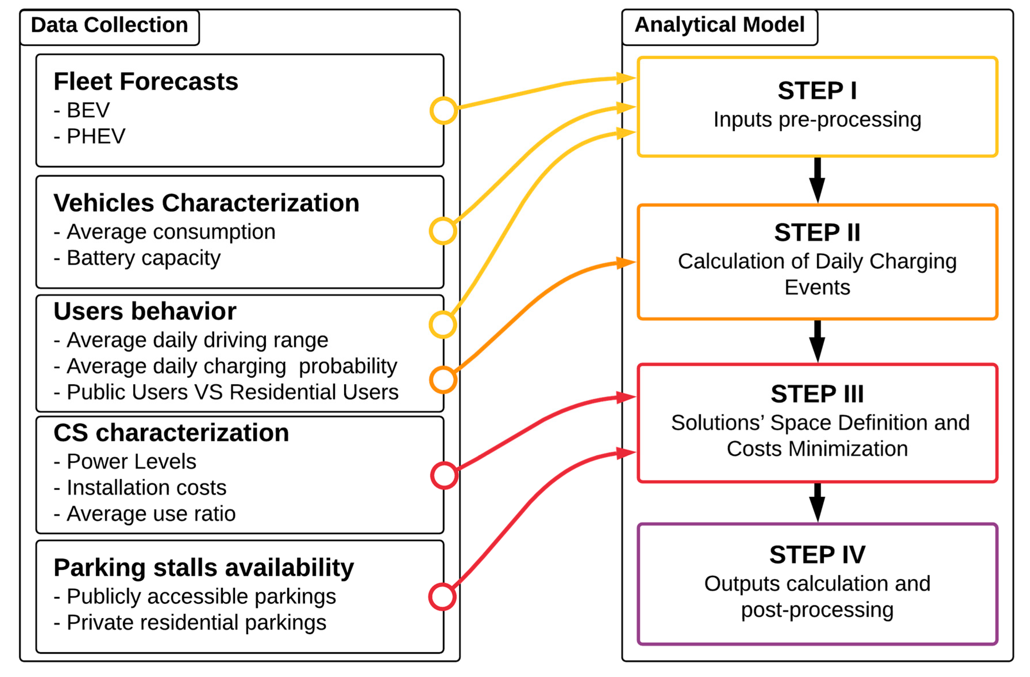
2.2.1. Data Collection

This section describes all the necessary inputs, as well as the data collection methods, while Section 3.1 reports the specific values of the actual data used during model implementation, together with a description of the data sources. The data collected can be classified under five macro-categories, spanning from BEV and PHEV fleets size forecast, to their average range and consumption; from parking spaces availability to users’ behaviors and finally to CS characteristics and costs.

BEV and PHEV fleets forecast over the analysis timeframe:

As already specified in the introduction, only the M1 category light passenger car sector would be considered in this paper. According to [24], M1 category vehicles are designed and constructed for the carriage of passengers, comprising no more than eight seats in addition to the driver’s seat. A literature research was then carried out for forecasts on BEV and PHEV car fleets size, over the 2020–2030 period, with a specific focus in years 2020, 2025 and 2030 and referring to the two evaluated areas. Unfortunately, no municipality-level results were publicly available, thus the research was further extended to forecasts evaluating single EU countries, as well as the EU-28 region as a whole. Following this decision, a methodology to scale down National and EU-28-level data back to the context of a municipality was then developed. In order to check dataset soundness for model’s scopes, the methodology also compares the collected forecasts to the existing market conditions, using the EU-28 global passenger car fleet turnover rate as a threshold for xEV fleet forecast growth rate.

Being the xEV market relatively new and still evolving, it presents different penetration levels across EU countries; this situation can be related to local factors such as the current development of the charging infrastructures and the existence (or the lack) of active support schemes and subsidies. On the other hand, the total passenger vehicle market—mainly composed by ICEV—is well-developed and with a relatively stable trend in terms of number of circulating vehicles. Following the previous considerations, the methodology has been developed under two main assumptions:

• Within 2050, the xEV distribution across EU-28 countries will follow that of total passenger fleet.
• The forecasts downscaling is realized sequentially: from EU-28 level to national level, then from the national level to municipality level.

As the first step of the process, a baseline of auxiliary information is defined for each of the three geographical levels, to be used by the transfer formulas during dataset downscaling. It is composed by an historical dataset, evaluated over the 2012–2017 period and composed by four specific entries:

• Total circulating fleet (ICEV, BEV and PHEV): TOT;
• Total circulating xEV (BEV and PHEV): xEV;
• Total new vehicles registrations (ICEV, BEV and PHEV): NR_TOT;
• Total new xEV registrations: NR_EV.

The last two variables, namely new vehicles and new xEV registrations, were selected as control parameter to check the soundness of the total circulating fleet and total circulating xEV data. Moreover, the auxiliary baseline comprises a forecast value of 2050 total circulating fleet (TOT), obtained by literature research.

After this preparation phase, the downscaling process of the xEV fleet forecasts was performed with the following procedure (the ‘input’ subscript refers to the geographical area analyzed by the forecast; the ‘output’ subscript refers to the geographical area to which the forecast was being scaled to):

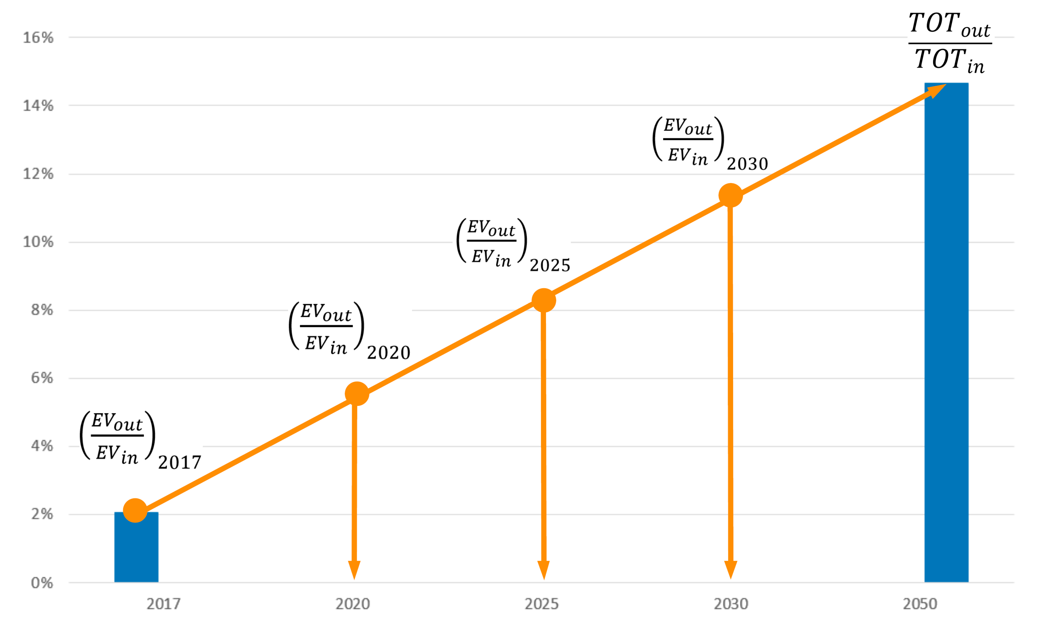
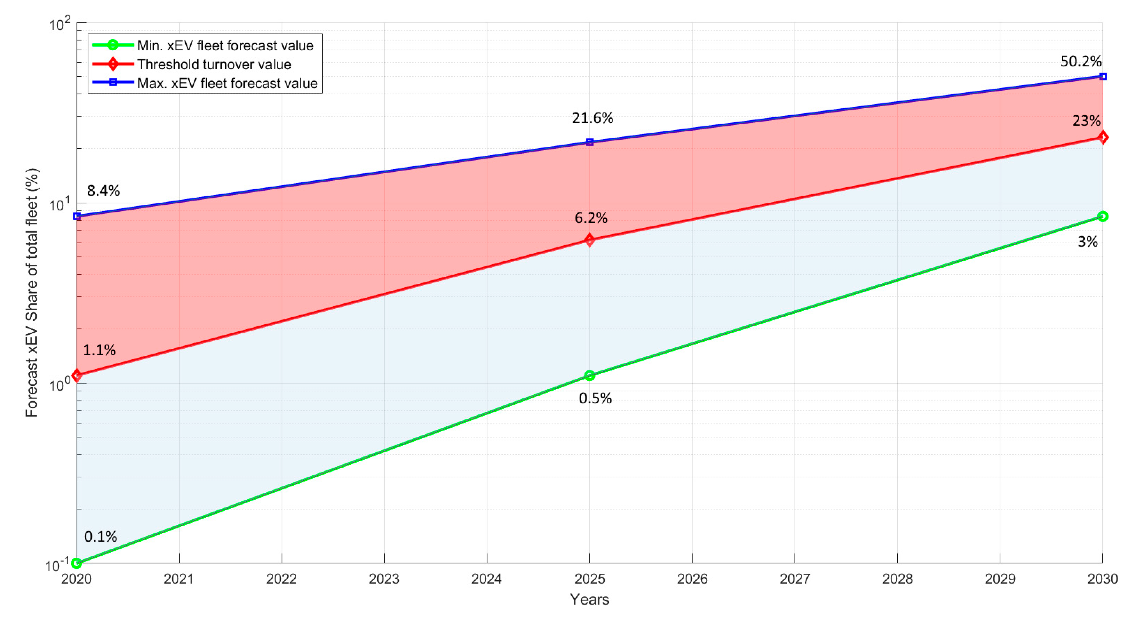
• At the starting year, i.e., 2017, the historical value of ${\left(\frac{xE{V}_{output}}{xE{V}_{input}}\right)}_{2017}$, which expresses the ratio between the xEV fleet circulating in the two considered areas (i.e., EU-28 and Italy), was assumed.
• At 2050, ${\left(\frac{xE{V}_{output}}{xE{V}_{input}}\right)}_{2050}$ was assumed equal to ${\left(\frac{TO{T}_{output}}{TO{T}_{input}}\right)}_{2050}$, which expresses the ratio between the total circulating car fleets forecast in the two considered areas.
• Finally, ${\left(\frac{xE{V}_{output}}{xE{V}_{input}}\right)}_Y$ was related to the Y-th year of the considered time period and was calculated under the assumption of a linear behavior, as described in Figure 2.

Once the forecasts for the xEV fleets size were scaled down to the municipality level, the resulting values were compared, for every year of the period, with a threshold value $T{h}_y$, calculated as following:

$$T{h}_y={\displaystyle \sum _{i=1}^y\left[To\ast {\left(shar{e}_{xEV}\right)}_i\ast TO{T}_i\right]},$$

(1)

where $To$ is the average EU-28 car fleet yearly turnover, with a value of 5.4% [25,26] and ${\left(shar{e}_{xEV}\right)}_i$ is defined as the xEV share of the EU-28 yearly car turnover, variable over 2020–2030 the period and assuming the values shown in

Table 1. Assumed xEV share of EU-28 yearly car turnover for the various years of the analyzed timeframe.

	2020	2025	2030
xEV share of EU-28 yearly car turnover	5%	15%	50%

. Currently, the share of xEV in the annual turnover equals 0.24% for Italy (2017 data) and stays below 4% for most of the European countries [13]; however, it has to be considered the impact that incentives and policies may have on the development of the EV market and the high probability of being activated in the period considered by this study, as highlighted by [13].

Finally, $TO{T}_y$ defines the forecast total circulating fleet (ICEV, BEV and PHEV) on the y-th year of period.

A specific forecast was used in the following steps only if all its values were below the threshold, otherwise it was discarded. The equation used for evaluation is described below:

$$xE{V}_y\le T{h}_y\forall y\in \left(timeperiod\right).$$

(2)

Finally, the remaining municipality level forecasts were used to define three scenarios for each municipality considered, using the following criteria:

• Low Scenario: it uses the lowest value of all the selected forecasts for every year of the time period.
• Medium Scenario: it uses an average value calculated from the values of all the selected forecasts for every year of the time period.
• High Scenario: it uses the highest value of all the selected forecasts for every year of the time period.

Average BEV and PHEV energy consumption and batteries capacity:

Average xEV consumption (expressed in kWh km⁻¹) and battery capacity (expressed in kWh) has been considered as a variable, to reflect the inevitable technological advances that will take place over the analyzed period. The values attributed for the year 2020 were obtained from the analysis of the current BEV and PHEV fleet [27] average consumption—measured using WLTP cycle estimations [28]—and capacity of the battery pack.

More specifically, the capacity of the battery pack assigned for the first year of analysis timeframe has been defined as the average of the capacities of the 15 best-seller M1-class BEV (and PHEV), weighted by sales volumes [29]. In order to consider the actual battery discharging capacity the obtained values have been reduced by 30% [28], then assigned to variables ${\left(bat{t}_{PHEV}\right)}_{2020}$ and ${\left(bat{t}_{BEV}\right)}_{2020}$.

The same approach was also used to define the average mean BEV consumption ${\left(av{c}_{BEV}\right)}_{2020}$, while to obtain the average mean PHEV consumption ${\left(av{c}_{PHEV}\right)}_{2020}$ a further step was required, since their typical use involves the simultaneous operation of both thermal and electric motor. A literature study shown that on average PHEVs cover about 32%–55% of their mileage using electric energy taken from the grid [30]; another approach, presented in [31], suggests an electric load reduction of about 50% compared to BEV vehicles. With a view to make the model easier to implement, the approach of [31] was chosen to define the ${\left(av{c}_{PHEV}\right)}_{2020}$ value, thus defined as the half of ${\left(av{c}_{BEV}\right)}_{2020}$.

On the upper end of the timeframe, namely 2030, these variables were estimated through literature research ([32,33] for consumption and [31,34] for battery capacities). The figures for the remaining years of the period were obtained as linear interpolation of the two extremes.

Public and private stalls availability:

The objective was to assess the availability of adequate space for the installation of private and publicly accessible CS, with a view to define upper limits to the planned charging infrastructure and to allow the evaluation of its impact on stalls occupation.

The following input variables were defined: public parking stalls available on Florence and Bruxelles areas $P{P}_{FI}$, $P{P}_{BXL}$ and private residential parking available on Florence and Bruxelles areas $P{R}_{FI}$, $P{R}_{BXL}$. Data has been collected through research on an existing database; all these variables are defined as constant during the evaluated period.

CS characteristics definition:

The proper functioning of the model requires the characterization of the charging infrastructure in terms of:

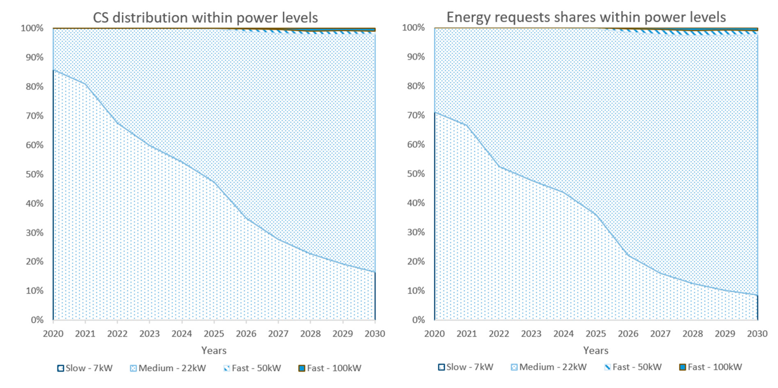
• Charging power levels ${\left(P_k\right)}_y$: the number of power levels and the related power outputs are defined after literature research; private residential and publicly accessible CS are accounted separately.
• Capital costs of the various types of CS ${\left(C_k\right)}_y$: they take into account CS cost, installation and grid connection costs; operation and maintenance costs are not considered.
• Estimated utilization rate of the various types of CS ${\left(r_{k,j}\right)}_y$: it is expressed in terms of the maximum number of charging events manageable by the CS on an average daily basis. They depend on the assumed daily usage timeframe $h_k$, on the charging power level ${\left(P_k\right)}_y$ and on the energy request of the charging event $E_j$; subscript k relates to the power level, while subscript j relates to the charging energy request class. They are calculated by comparing the hours of assumed daily availability with the time needed for a charge:

  $$\left(r_{k,j}\right)=\frac{h_k}{\left(\frac{E_j}{{\left(P_k\right)}_y}\right)}.$$

  (3)

The values assumed by these three variables can be updated during the analyzed period; within this study the same values were used for each analyzed municipality.

Driving and charging behavior of users:

The driving and parking habits of users, together with the way they are expected to use the EV charging infrastructure, have a great impact on its characterization, and thus on model outputs. A set of three variables was implemented in order to describe this scenario:

• Average daily driven distance: A literature research focused on urban areas did not return appropriate results, so national level values were used. Anyway, given the fact that urban travels are shorter than the average, the data used was more conservative in terms of energy request to the infrastructure. The values were considered as constant over the timeframe, but differentiated within the two considered areas: $av{d}_{FI}$ and $av{d}_{BXL}$.
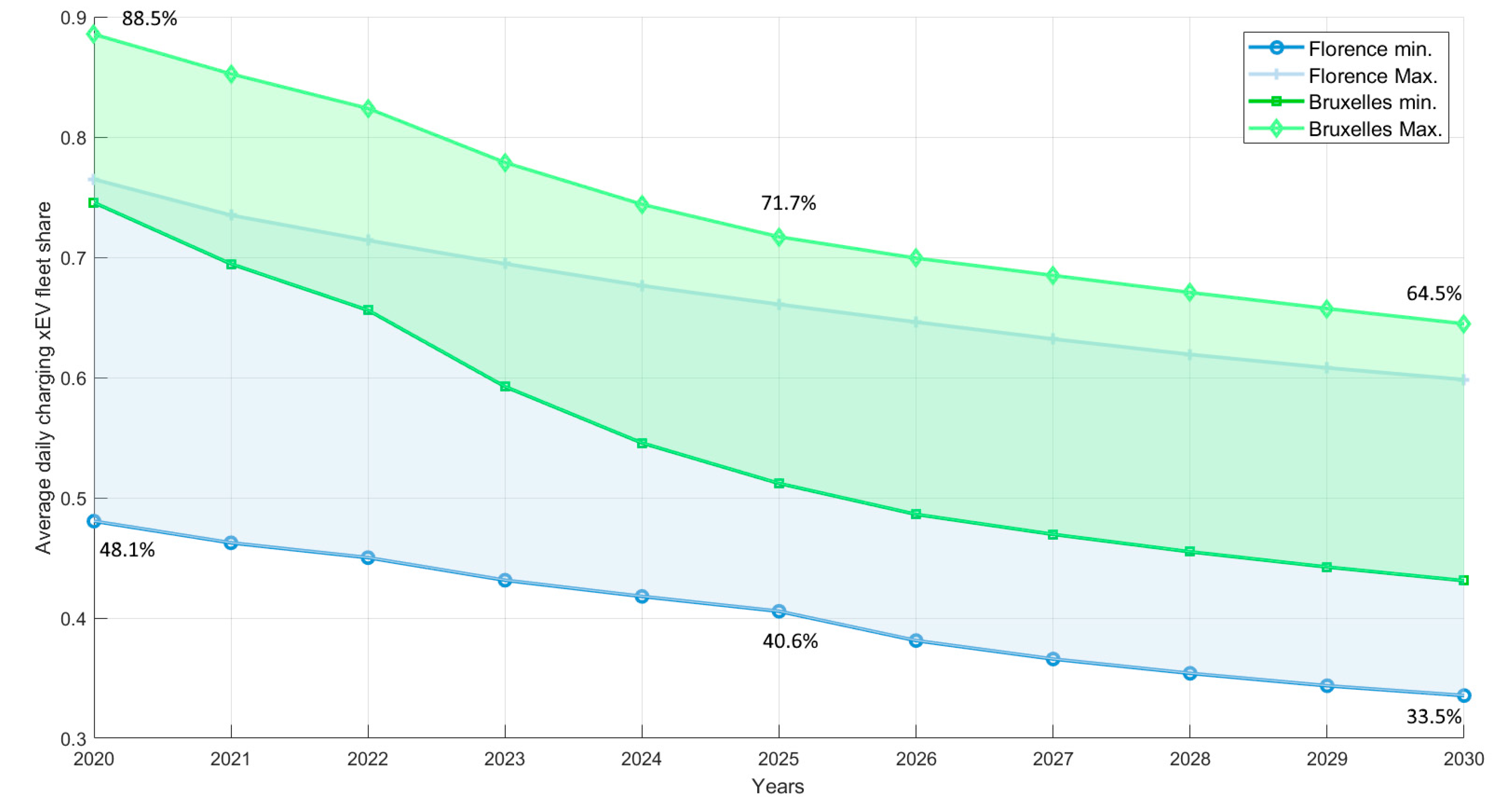
• Use of publicly accessible or private residential CS: It is crucial to estimate the share of BEV and PHEV that will weigh on average on the public charging infrastructure; therefore, a literature research has been carried out in order to estimate the percentage of BEV and PHEV that will use the public charging infrastructure over the y-th year of the period: ${\left(\%BE{V}_P\right)}_y$ and ${\left(\%PHE{V}_P\right)}_y$.
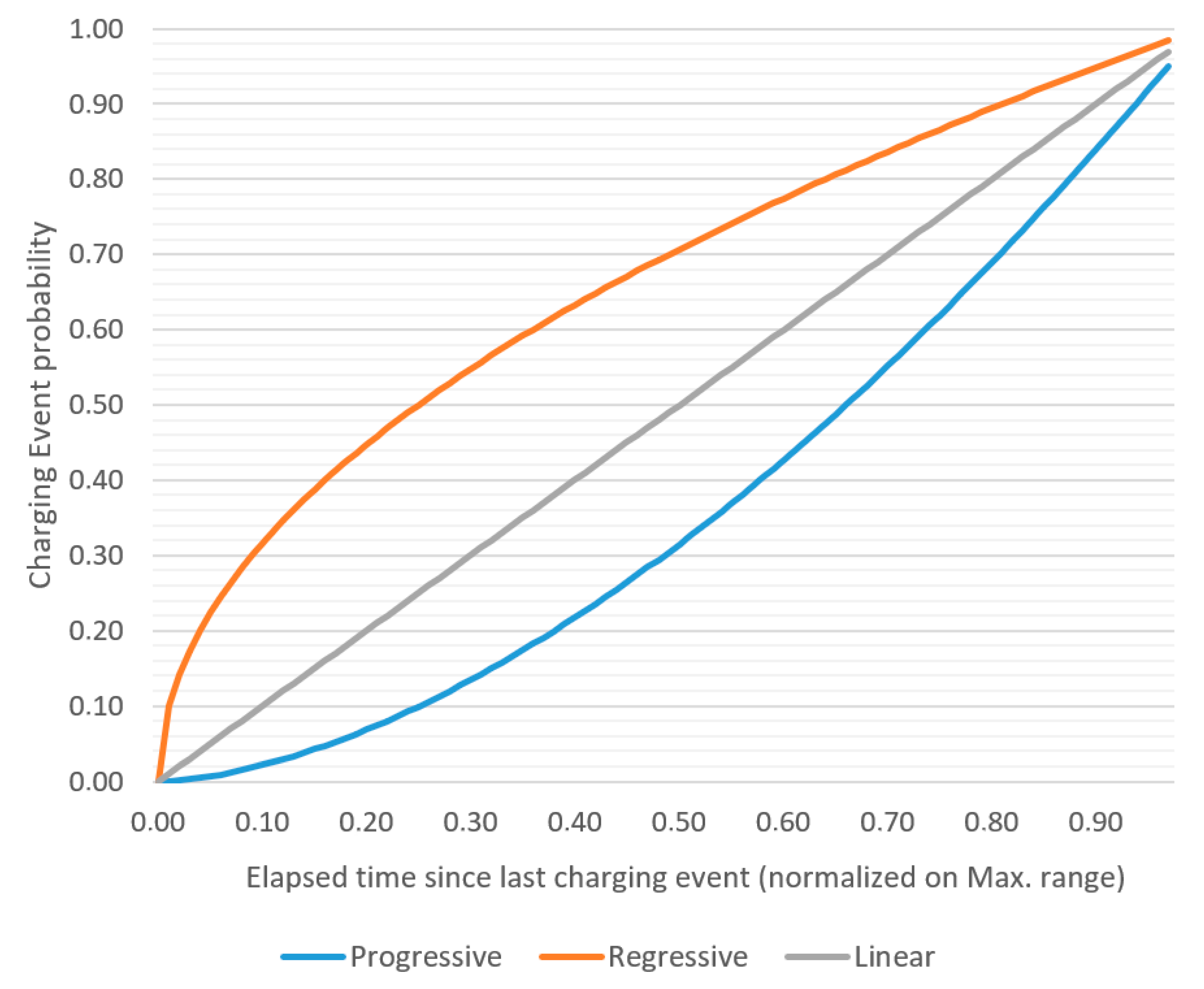
• Charging events probability distribution over the estimated range of the vehicle: Usually xEV driving range allows for more than one day of use so owners can decide to charge their vehicles when state of charge (SOC) approaches the minimum level or before. This consideration, together with the hypothesis of only complete recharges, leads to different possible energy requests for the single charging event. Thus, it was necessary to develop a methodology to distribute the probability of the charging events over the whole driving range allowed by the battery size. Since this situation is strongly related to user behavior modeling, in order to cover the various possibilities, three different scenarios have been developed, each with a specific probability distribution over the timeframe. The independent variable is represented by the time elapsed since the last charging event (normalized to the maximum autonomy) and is therefore included in an interval [0,1]; the dependent variable p is the probability of a charge event at a given time, defined as a monotonous increasing function with its values included in the interval [0,1]. Immediately after a charging event p = 0, while at the end of the driving range p = 1, thus avoiding the possibility that a xEV runs out of charge. Figure 3 shows the trends of the three functions defining the different scenarios.

2.2.2. I Step: Input Pre-Processing

Some of the inputs described in the previous section have direct use in the model, while others need to be further processed. More specifically, the forecasts on BEV and PHEV fleets sizes through the analyzed timeframe were collected as inputs; the model will evaluate separately the number of BEV and PHEV charging using publicly accessible infrastructure from the ones that will use private residential infrastructure, so the following new variables have to be defined:

$$\{\begin{array}{l}{\left(BE{V}_P\right)}_y={\left(\%BE{V}_P\right)}_y\ast {\left(BEV\right)}_y\\ {\left(BE{V}_R\right)}_y=\left[1-{\left(\%BE{V}_P\right)}_y\right]\ast {\left(BEV\right)}_y\\ {\left(PHE{V}_P\right)}_y={\left(\%PHE{V}_P\right)}_y\ast {\left(PHEV\right)}_y\\ {\left(PHE{V}_R\right)}_y=\left[1-{\left(\%PHE{V}_P\right)}_y\right]\ast {\left(PHEV\right)}_y\end{array},$$

(4)

where ${\left(BE{V}_P\right)}_y$ and ${\left(PHE{V}_P\right)}_y$ refers to the shares charging on public infrastructure and ${\left(BE{V}_R\right)}_y$ and ${\left(PHE{V}_R\right)}_y$ refers to the shares charging on private residential infrastructure, both over the y-th year of the time period.

Finally, in order to define xEV range as the maximum allowable period of time (measured in days) between two successive charging events, it has to be defined the new variable ${\left[{\left(av{r}_V\right)}_A\right]}_y$ as:

$${\left[{\left(av{r}_V\right)}_A\right]}_y=\frac{{\left(bat{t}_V\right)}_y}{{\left(av{c}_V\right)}_y\ast av{d}_A},$$

(5)

where subscript A refers to the geographical area, V to the type of vehicle (BEV or PHEV) and y to the y-th year of the timeframe. This general notation will be used in the following sections of this document.

2.2.3. II Step: Calculation of Daily Charging Events on Publicly Available Infrastructure

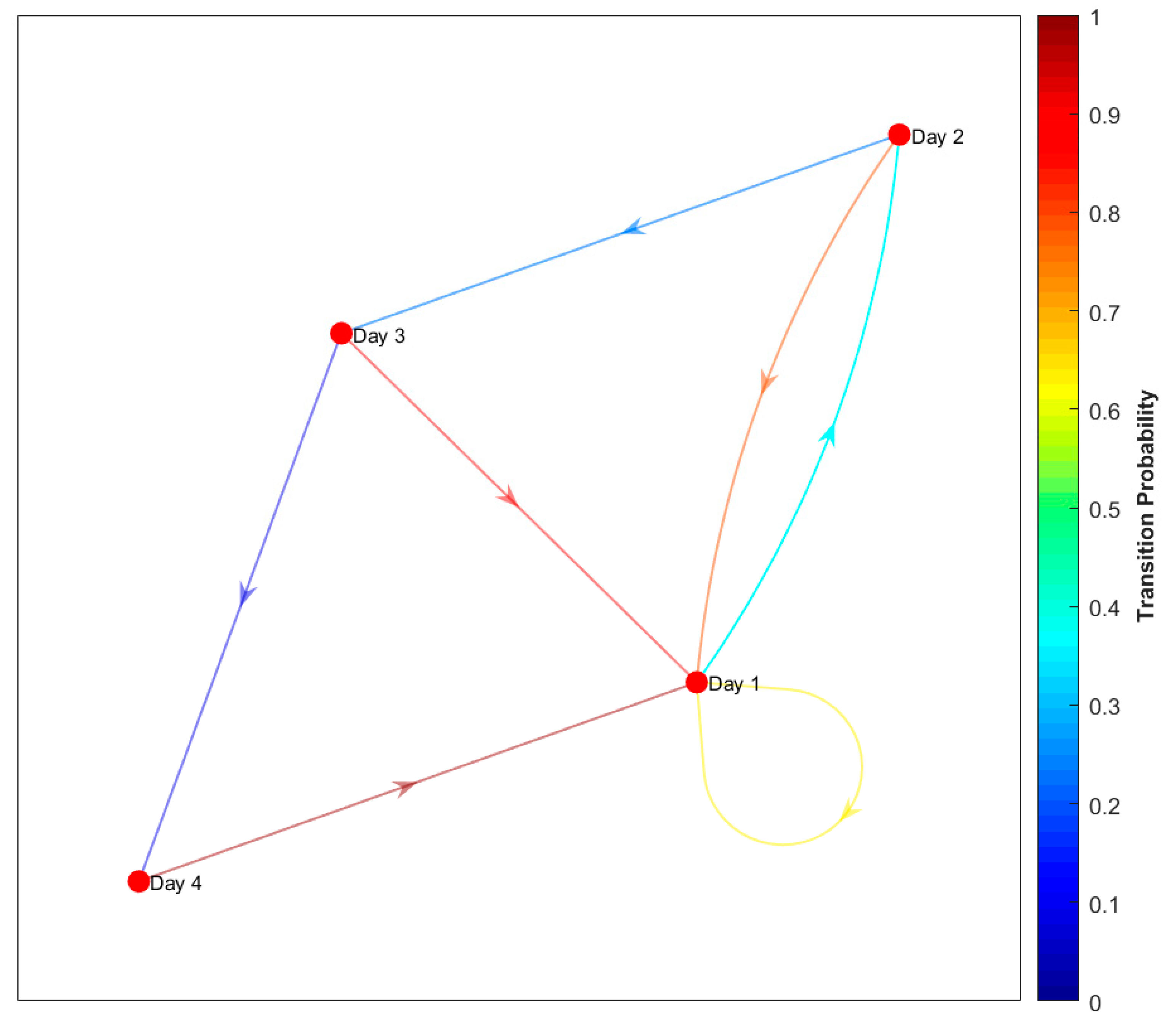
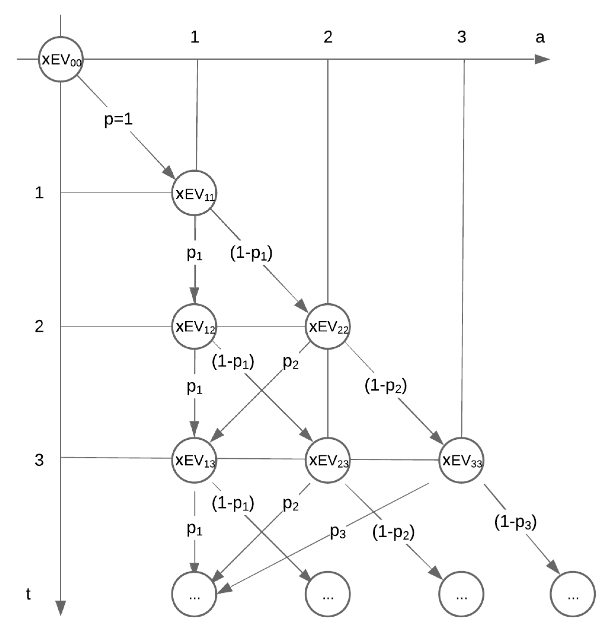
In this step of the model the average number of daily charging events related to the BEV and PHEV circulating fleet is calculated, together with the corresponding energy requests. To do so, the average number of daily charging vehicles and their SOC at the beginning of the charge have to be estimated. BEV and PHEV have different electric driving ranges, thus they are separately evaluated within the model; anyway, since the operations are conceptually identical, in the followings of this section we would simply refer to xEV without losing generality. A discrete-time Markov chain (DTMC), applied to a countable, finite state-space was used to obtain the estimate of the average daily distribution of the SOC levels within the xEV circulating fleet. The DTMC is defined by the transition matrix $\left[A\right]$, which values are obtained by applying the charging events probability distribution p over the specific driving range considered, with a 1-day timestep:

$$\left[A\right]=\left(\begin{array}{ccccc}{p}_1& \left(1-p_1\right)& 0& \cdots & 0\\ p_2& 0& \left(1-p_2\right)& \cdots & 0\\ ⋮& ⋮& ⋮& \ddots & ⋮\\ p_{n-1}& 0& 0& \cdots & \left(1-p_{n-1}\right)\\ p_n=1& 0& 0& \cdots & 0\end{array}\right).$$

(6)

The transition matrix defines the charging probability of a xEV for each day of the driving range; once the driving range ${\left[{\left(av{r}_V\right)}_A\right]}_y$ is defined, also the dimension of the state-space and of the transition matrix $\left[A\right]$ are set accordingly. Figure 4 shows an example of DTMC graph, applied to a 4-days driving range scenario.

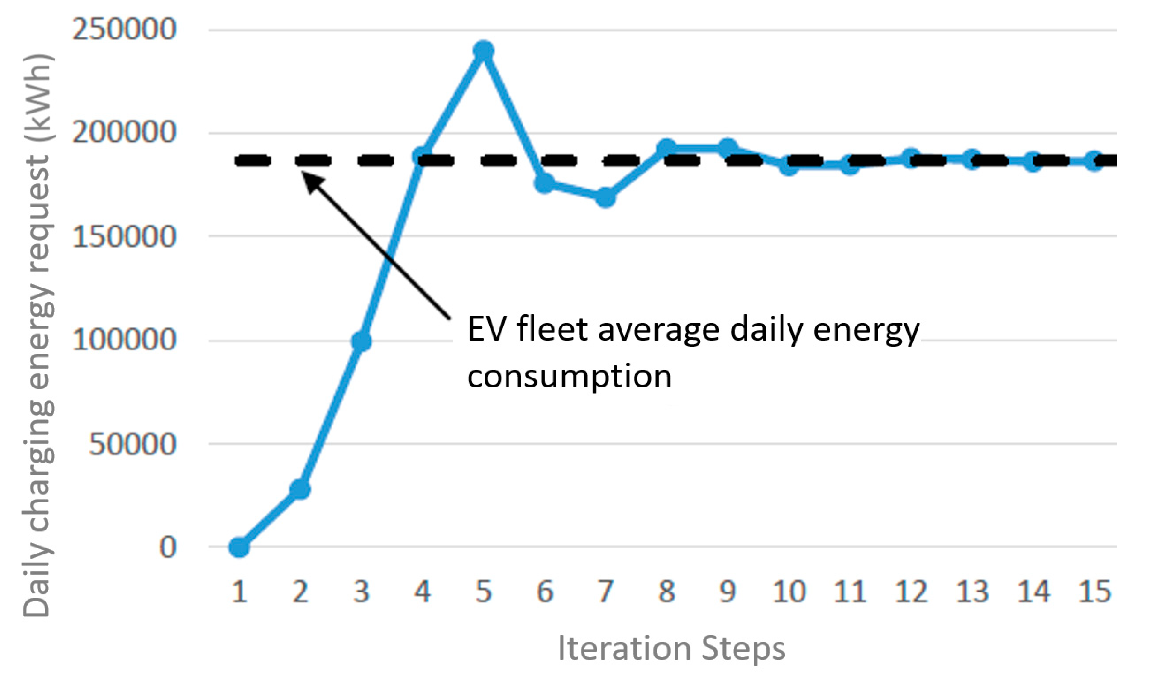
The evolution of the DTMC is calculated with an iterative process—highlighted by Figure 5—that usually reached convergence within 15 steps. The final stationary probability distribution describes the average distribution of SOC levels within the xEV circulating fleet. The application of the transition matrix $\left[A\right]$ to this stationary distribution, finally allows us to stochastically define the average number of xEV daily charging, for each SOC level.

The horizontal axis represents timesteps “a”, which are inscribed within the interval $\left[0,{\left[{\left(av{r}_V\right)}_A\right]}_Y\right]$, while the vertical axis represents the iteration steps. A different SOC is associated to every timestep “a”, thus a different charging energy request; taking into account the hypothesis of only complete charges its value $E_a$ can be calculated as:

$${\left[{\left(E_a\right)}_V\right]}_y={\left[{\left(av{c}_V\right)}_A\ast av{d}_A\right]}_y\ast a.$$

(7)

The output is then a series of couples $\left(xE{V}_a,E_a\right)$, dividing the charging xEV in different groups in terms of energy requests.

In order to check the stability of the iterative process and the quality of the results, two control methods were implemented:

• The sum of the elements $a_{i,j}$ for each row of the transition matrix $\left[A\right]$ must be equal to one, since they define all the possible transition events completely:

  $${\displaystyle \sum _{j=1}^j{a}_{i,j}=1}.$$

  (8)
• The total energy recharged by infrastructure (after convergence) must be equal to the average energy consumed by the xEV fleet using public charging infrastructure (Figure 6):

  $${\left[{\left(xE{V}_P\right)}_A\right]}_y\ast {\left[{\left(av{c}_V\right)}_A\ast av{d}_A\right]}_y={\displaystyle \sum _{a=1}^{{\left[{\left(a{m}_{xEV}\right)}_A\right]}_y}xE{V}_{a,t}\ast E_a},\forall t>\stackrel{-}{t},$$

  (9)

  where $\overline{t}$ is the convergence iteration step.

2.2.4. III Step: Publicly Available Infrastructure Solutions’ Space Definition and Costs Minimization

Single event charging energy requests $E_a$ are related to specific consumption ${\left[{\left(av{c}_V\right)}_A\right]}_y$ and to battery capacity ${\left(bat{t}_V\right)}_y$, thus they are different between BEV and PHEV; they also evolve during the time period. The overall range of variation of $E_a$ spans from zero to the maximum value of battery capacity ${\left(bat{t}_{BEV}\right)}_{2030}$; in order to simplify the model structure, this range has been divided in 10 equally spaced classes, each one with a constant energy value $E_j$, with:

$$\{\begin{array}{l}{E}_j=j\ast \frac{{\left(E_a\right)}_{\max }}{10}\\ E_0=0\end{array},1\le j\le 10.$$

(10)

Then, every $E_a$ value has been compared with $E_j$, so that for every $E_{j-1}\le E_a\le E_j$ the model apply the substitution $E_a=E_j$. This way, several different values of energy requests $E_a$ are reduced to only ten values of $E_j$; this assumption is safe since it always overestimates the energy requests. The couples $\left(BE{V}_a,E_a\right)$ and $\left(PHE{V}_b,E_b\right)$ are transformed into $\left(\left(BE{V}_j+PHE{V}_j\right),E_j\right)$, thus inscribing BEV and PHEV energy requests into the same framework and allowing us to use the additive and modular architecture that was one of the basic choices for the model.

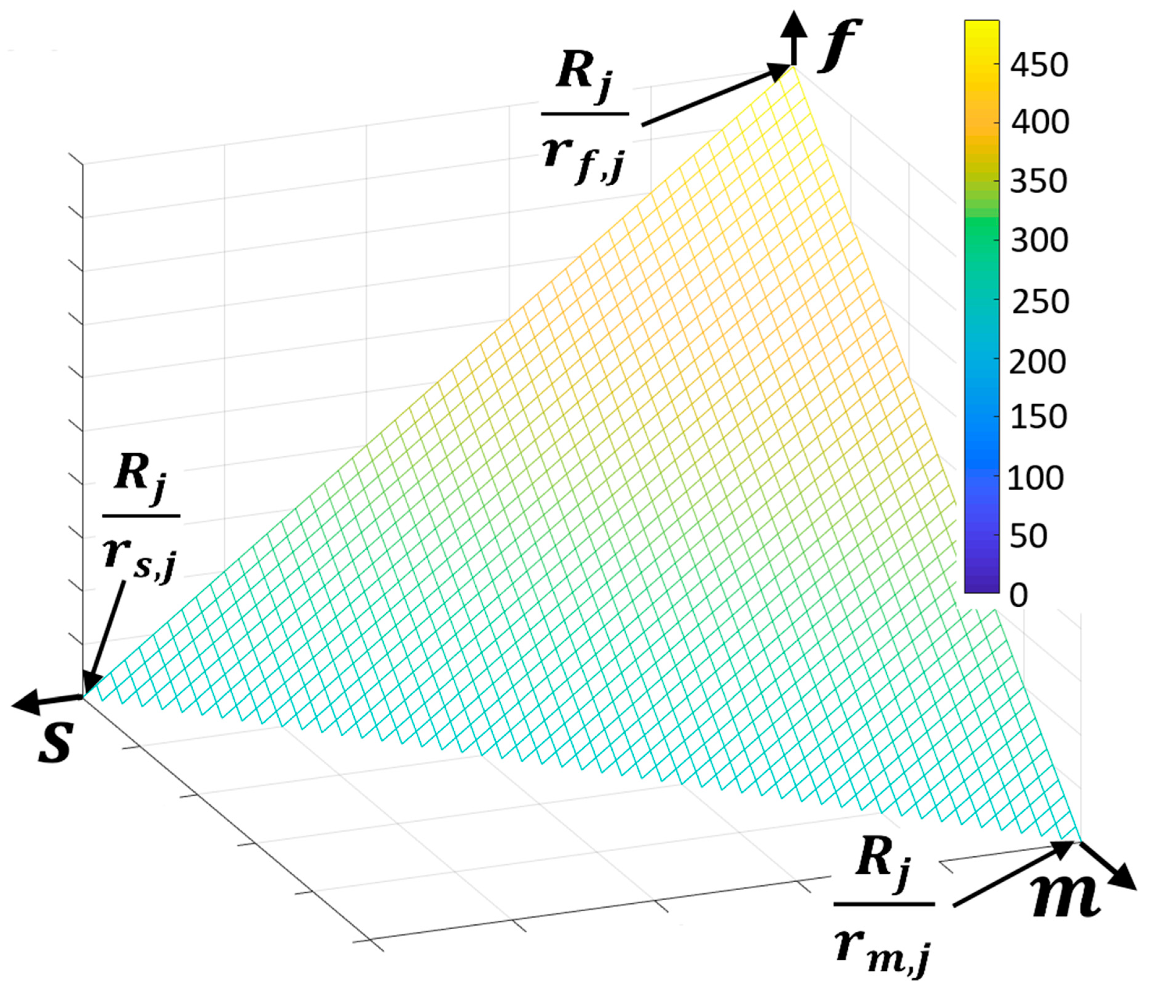
Given the modular architecture of the model, infrastructure size is calculated for every j-th class of energy requests and, after the cost optimization phase, the total value is obtained by summation. Since ${\left(r_{k,j}\right)}_y$ already takes into account charging energy requests, all the public infrastructure compositions that are able to satisfy the total number of daily charging events $R_j=\left(BE{V}_j+PHE{V}_j\right)$ are considered as suitable. The space of the solutions, for every j-th class, is a triangular portion of a plane, as Figure 7 shows, described by the following equations:

$$\{\begin{array}{l}{R}_j=r_{s,j}\ast s_j+r_{m,j}\ast m_j+r_{f,j}\ast f_j\\ s_j\ge 0\\ m_j\ge 0\\ f_j\ge 0\end{array},$$

(11)

where the triplets ${\left(s_j,m_j,f_j\right)}_n$ define all the n possible combinations of CS that satisfy total daily charging requests $R_j$.

After all the technically possible solutions are found, CS costs are applied, in order to optimize the system and find the least-cost solution for each energy level; this is done by searching the minimum value of the ${\left(C_{TOT,j}\right)}_n$ term of the equation:

$${\left(C_{TOT,j}\right)}_n=C_s\ast s_{j,n}+C_m\ast m_{j,n}+C_f\ast f_{j,n}, \forall {\left(s_j,m_j,f_j\right)}_n.$$

(12)

The outputs of this step are the minimum cost of a charging infrastructure suitable for the j-th class charging request and its composition in terms of CS:

$$\{\begin{array}{c}{\left(C_{MIN}\right)}_j\\ {\left(s_{MIN},m_{MIN},f_{MIN}\right)}_y\end{array},j\in \left[1,10\right].$$

(13)

2.2.5. IV Step: Output Definition

This final step is designed to aggregate the outputs coming from steps II and IV, and to post-process them with some of the inputs in order to obtain the other PI for the specific charging infrastructure. In this section the operations needed to accomplish the first goal will be described, while the results of the latter will be discussed in the next section.

BEV and PHEV daily charging on publicly available infrastructure:

The total number of xEV daily using the charging infrastructure during y-th year can be obtained by summation of the values related to every j-th level:

$$\{\begin{array}{c}{\left(BE{V}_P\right)}_y={\displaystyle \sum _{j=1}^{10}{\left(BE{V}_j\right)}_y}\\ {\left(PHE{V}_P\right)}_y={\displaystyle \sum _{j=1}^{10}{\left(PHE{V}_j\right)}_y}\end{array}.$$

(14)

Energy and power demand from publicly available charging infrastructure:

Couples of values ${\left(E_j,BE{V}_j\right)}_y$ and ${\left(E_j,PHE{V}_j\right)}_y$ are sufficient for the calculation of total energy provided by charging infrastructure during y-th year:

$${\left(E_{TOT}\right)}_y={\displaystyle \sum _{j=1}^{10}{\left(E_j\ast BE{V}_j\right)}_y+{\left(E_j\ast PHE{V}_j\right)}_y}.$$

(15)

In order to calculate the energy provided by each power level of the infrastructure, each of the j-th level contributions must be evaluated separately and finally summed:

$${\left[{\left(E_{TOT}\right)}_k\right]}_y={\displaystyle \sum _{j=1}^{10}{k}_{MIN,j}\ast E_j\ast r_{k,j}},k\in (s,m,f).$$

(16)

Publicly available charging infrastructure composition and cost:

The number of charging stations for the various CS power levels and their cost are provided as output for each y-th year and each j-th energy class by the equations state da the end of Section 2.2.4; total yearly values are obtained by a sum in j and total global values are the obtained by another sum in i:

$$\{\begin{array}{c}\left(C_{MIN}\right)={\displaystyle {\sum }_i{\displaystyle \sum _{j=1}^{10}{\left[{\left(C_{MIN}\right)}_j\right]}_y}}\\ \left(s_{MIN},m_{MIN},f_{MIN}\right)={\displaystyle {\sum }_i{\displaystyle \sum _{j=1}^{10}{\left[{\left(s_{MIN},m_{MIN},f_{MIN}\right)}_j\right]}_y}}\end{array}.$$

(17)

Energy and power demand from private residential charging infrastructure

The basic assumption regarding the use of private residential charging infrastructure is that each vehicle is assumed to be used and charged every day. This simplifying assumption is related to the fact that, being the stall private and related to the vehicle, this one will be parked there at least once in the day, ready to be charged. The equation describing the total average daily energy request is:

$${\left[{\left(E_r\right)}_A\right]}_y={\displaystyle {\sum }_V\left\{\left[1-{\left(\%xE{V}_P\right)}_y\right]\ast {\left(xEV\right)}_y\ast {\left(av{c}_V\right)}_y\ast av{d}_A\right\}}.$$

(18)

Private residential charging infrastructure cost:

The least cost for the private residential charging infrastructure is obtained using the following equation:

$${\left[{\left(C_r\right)}_A\right]}_y={\displaystyle \sum _{i=1}^y{\displaystyle {\sum }_V\left\{\left[1-{\left(\%xE{V}_P\right)}_y\right]\ast {\left(xEV\right)}_y\ast {\left(C_r\right)}_y\right\}}}.$$

(19)

The least cost assumption derives from the fact that no overlap in the use of publicly accessible and private residential charging infrastructure is modeled, while a certain share of it is expected.

2.3. Scenario Definition

A total of 18 working scenarios have been defined; they are the result of a three-step combination of various assumptions, as described below.

The first step is related to the two different geographical areas analyzed—here Florence and Bruxelles—and affects the following input variables:

• Average daily travel $av{d}_{FI}$ and $av{d}_{BXL}$.
• Publicly accessible stalls $P{P}_{FI}$ and $P{P}_{BXL}$.
• Private residential parking $P{R}_{FI}$ and $P{R}_{BXL}$.

The second step considers the three different xEV fleet forecast scenarios calculated for each geographical area, here defined as low, medium and high; it affects the following inputs variables:

• BEV circulating fleet on y-th year ${\left(BE{V}_{FI}\right)}_y$ and ${\left(BE{V}_{BXL}\right)}_y$.
• PHEV circulating fleet on y-th year ${\left(PHE{V}_{FI}\right)}_y$ and ${\left(PHE{V}_{BXL}\right)}_y$.

The final step is related to user behavior modeling and specifically to the charging events probability distribution over the estimated range of the vehicle p.

3. Results and Discussion

3.1. Input Values Definition for the Implemented Scenarios

In the following sections the specific input values used in the model for this study were described.

BEV and PHEV fleets forecast over analysis timeframe:

An historical dataset was needed as a baseline of auxiliary information for the development of the transfer formulas for dataset downscaling; the main sources for data collection are shown in

Table 2. Data sources for historical baseline characterization (FI = Florence, BXL = Bruxelles).

Source	EU-28	IT	BE	FI	BXL	Data
Centro Studi Continental A [35]	-	-	-	X	-	$\frac{E{V}_{FI}}{E{V}_{IT}}$
Comune di Firenze [36]	-	-	-	X	-	TOT
EAFO [26]	X	X	X	-	-	NREV
ECOSCORE B [37]	-	-	X	-	X	TOT, EV
ENEL e-mobility [14]	-	X	-	-	-	EV
Eurostat [19]	X	X	X	-	-	NTOT, NEV
IBSA [38]	-	-	X		X	TOT, EV
UNRAE [39]	-	X	-	-	-	NRTOT, NREV

^A: Author’s elaboration on ACI data; ^B: owned by Vito.be.

, with a reference to the area considered.

Table 3. Data sources for xEV fleet size forecasts.

Source	Paper	Analyzed Area	Release Year	Proposed Scenarios
				N.	2020	2025	2030
Eurelectric *	Smart Charging: steering the charge, driving the change [40]	EU-27	2015	3	X	X	X
Delft-CE	Impact analysis for market uptake scenarios and policy implications [41]	EU-27	2011	3	X	X	X
RSE	Roadmap per una mobilità sostenibile [42]	IT	2017	1	X	X	X
Start/CEI CIVES	Libro Bianco EV [43]	IT	2017	4	X	-	-
EAFO	The transition to a Zero Emission fleet for cars in the EU by 2050 [26]	EU-28	2016	3	X	X	X
ENEL/Ambrosetti	E-Mobility Revolution [14]	IT	2017	4	-	X	X
PoliMi	E-Mobility report 2018 [13]	IT	2018	3	X	X	X
ENTSO-E	TYNDP 2018 [44,45]	IT, BE	2018	3	X	X	X
European Commission	Clean Power for Transport [46]	IT, BE	2017	3	X	X	X

*: 2020 to 2030 data obtained by linear interpolation.

highlights the sources used to collect the forecast data for xEV fleets growth. Since only [13,26,39] reported separately the contribution of BEV and PHEV, an average value of the allocation suggested by those papers has been used to divide the other forecast data between BEV and PHEV contributions.

A total of 23 scenarios, from nine different studies was thus selected. Then these were compared to the maximum assumed turnover for xEV, as described in Section 2.2.1 and only the ones that were proposing forecasts lower than the maximum assumed turnover for xEV were used in the model. After this step, 11 scenarios from seven sources remained; Figure 8 shows the results in terms of xEV shares over the total circulating fleet, for Florence municipality. It also highlights the portion of scenarios range that overcame the selecting threshold.

Finally,

Table 4. Battery electric vehicle (BEV) and plug-in hybrid electric vehicle (PHEV) fleet forecasts for the area of Florence and Bruxelles municipalities—absolute figures.

Area	Scenario	BEV			PHEV
		2020	2025	2030	2020	2025	2030
Florence	Low	73	441	2062	90	517	2544
	Medium	202	1414	6344	584	2980	9886
	High	672	3968	14,030	1141	6016	21,532
Bruxelles	Low	663	3482	10,334	984	3482	12,168
	Medium	1283	6022	18,432	2655	10,266	25,451
	High	2689	10,078	35,836	5152	17,591	45,337

highlights the forecasts for BEV and PHEV circulating fleets during the considered time period, used in the model as inputs for this research.

Table 5. BEV and PHEV fleet forecasts for the area of Florence and Bruxelles municipalities—shares of total circulating fleet.

Area	Scenario	BEV			PHEV
		2020	2025	2030	2020	2025	2030
Florence	Low	0.0%	0.2%	1.0%	0.0%	0.3%	1.3%
	Medium	0.1%	0.7%	3.2%	0.3%	1.5%	5.0%
	High	0.3%	2.0%	7.0%	0.6%	3.0%	10.8%
Bruxelles	Low	0.1%	0.7%	2.1%	0.2%	0.7%	2.5%
	Medium	0.3%	1.2%	3.7%	0.5%	2.0%	5.2%
	High	0.5%	2.0%	7.3%	1.0%	3.4%	9.2%

shows the same data but this time in terms of shares of the total circulating fleets in the two selected areas.

Average BEV and PHEV energy consumption and capacity of batteries:

Table 6. xEV average consumption and capacity assumed forecast values.

	2020		2030
	BEV	PHEV	BEV	PHEV
Average specific consumption (kWh km−1) ${\left(av{c}_V\right)}_y$	0.192	0.108	0.154	0.086
Average battery useful capacity (kWh) ${\left(bat{t}_V\right)}_y$	31.6	7.14	59.5	9.8

shows the results obtained by applying the methodology described in Section 2.2.1 and subsequently applied in the model.

Public and private stalls availability:

In order to obtain the results highlighted in

Table 7. Public and private stalls availability in the analyzed areas of Florence (2013 data) and Bruxelles (2018 data).

	$\mathbf{Public}\mathbf{Stalls}\left(\mathit{P}{\mathit{P}}_{\mathit{A}}\right)$	$\mathbf{Private}\mathbf{Residential}\mathbf{Parkings}\left(\mathit{P}{\mathit{R}}_{\mathit{A}}\right)$
Florence	65,000	55,800
Bruxelles	318,600	293,000

the following sources were investigated:

• For the Florence area, open-data maps and databases developed by the municipality were used to assess public parking spaces availability [47], while the results of the 2011 census [48] were used to evaluate private residential parking spaces.
• With regards to the Bruxelles area, open-data databases were used to obtain the number of public parking spaces available, together with an estimate of private parking spaces in the residential area [49].

Definition of CS characteristics:

As a first step in choosing the implemented CS power level a research within existing National Regulations and EU-28 Directives has been performed, in order to gather suggestions and any provided prescription. The main sources consulted here were Directive 2014/94/EU [4] and the PNire [5].

Another research has then been performed to understand the current composition of publicly accessible charging infrastructures in the study areas, using accessible databases such as official open-data archives of municipalities [50], data from a service provider (Enel) [51] and other unofficial archives (Opencharger) [52], to understand the current composition of the infrastructure in terms of quantity, power levels and connection standards used.

The home charging sector has also been considered, evaluating the average installed power as well as the maximum that can be installed by a European household, to define an upper limit value for the power of the recharging system [53]. In conclusion, a literature research was carried out in order to evaluate the possible future developments of the infrastructure in terms of power levels and usage [34].

At the end of the research phase, the following power values were identified for the various charging systems used in the model, and finally applied both to Florence and Bruxelles area:

• Private residential charging points P_r: 2 kW
• Publicly accessible charging points: Three power levels and corresponding charging systems, called slow, medium and fast, have been implemented. The selected power values are listed in the following

  Table 8. Charging power levels assumed in the model for this study.

  Power Levels	Charging Power
  	2020–2024	2025–2030
  Slow—${\left(P_s\right)}_y$	7 kW	22 kW
  Medium—${\left(P_m\right)}_y$	22 kW	50 kW
  Fast—${\left(P_f\right)}_y$	50 kW	100 kW

  :

An installation cost has been defined for each CS power level; this value includes the cost of the charging station, including installation and grid connection costs. Operating costs were not considered, as they were not part of the scope of the study, nor were maintenance costs; the latter were not implemented in order maintain the model simple enough.

Learning curves were applied to capital, installation and connection costs, to take into account the reduction of costs over time related to the effects of industrialization and rationalization of processes. All the information derives from an extensive literature research (cfr. [10,31,41,46,54,55]) and brought to the definition of ${\left(C_s\right)}_y$, ${\left(C_m\right)}_y$, ${\left(C_f\right)}_y$ and ${\left(C_r\right)}_y$, related to the y-th year and described in

Table 9. Charging station (CS) costs forecast for the various power levels.

	2020	2025	2030
Private Residential—2kW ${\left(C_s\right)}_y$	900 €	810 €	729 €
Slow—7 kW ${\left(C_m\right)}_y$	1783 €	1630 €	1630 €
Medium—22 kW ${\left(C_f\right)}_y$	4800 €	4264 €	4264 €
Fast—50/100 kW ${\left(C_r\right)}_y$	44,000 €	38,798 €	32,564 €

.

A literature search was then carried out to verify the actual use ratios of existing charging infrastructures [20,56]. The driving and parking behaviors and daily timeframes of an average user were mainly derived from the study [23], which specifically analyses driving behavior in various European countries, including Italy. The results of these evaluations, together with other usage constraints and the energy request levels $E_j$, brought to the maximum number of charging events for level of energy requests reported in

Table 10. Maximum number of charging events daily manageable by each level of energy requests, for each Charging energy request class.

CS Power Levels		$\mathbf{Charging}\mathbf{Energy}\mathbf{Request}\mathbf{Classes}—{\mathit{E}}_{\mathit{j}}\left(\mathbf{kWh}\right)$
		6	12	18	24	30	36	42	48	54	60
2 kW	$r_{r,j}$	1	1	1	0	0	0	0	0	0	0
7 kW	$r_{s,j}$	3	3	3	2	2	2	2	2	2	0
22 kW	$r_{m,j}$	8	8	8	4	4	4	4	3	3	3
50 kW	$r_{f,j}$	12	12	12	12	8	8	8	8	4	4
100 kW	$r_{f,j}$	17	17	17	12	12	12	12	8	8	8

for each power level of the CS:

Driving and charging behavior of users:

For what it concerns the average daily travelled distance, two different values have been calculated, for Florence and Bruxelles, as shown in

Table 11. Forecast average daily travelled distance by a passenger car over the analyzed areas.

	Florence	Bruxelles
Average daily travelled distance (km) $\left(av{d}_A\right)$	23.5	30.5

the most recent data available (2015) have been used, from:

• Odyssee-Mure Database [57]: Italy and EU-28.
• ACEA [58]: Belgium.
• ACI—CENSIS [59]: Italy.

The shares of PHEV and BEV, which are considered as using the publicly accessible charging infrastructure, were calculated using data coming from [31,60]; the results are reported in

Table 12. Share of PHEV and BEV expected to be using the publicly accessible charging infrastructure.

	2020	2025	2030
Share of BEV using the publicly accessible charging infrastructure ${\left(\%BE{V}_P\right)}_y$	56.5%	66.9%	75.8%
Share of PHEV using the publicly accessible charging infrastructure ${\left(\%PHE{V}_P\right)}_y$	45.6%	58.6%	69.7%

:

Finally, the charging events probability distribution $p$ over the estimated range of the vehicle, was defined for three different scenarios (see Figure 3):

• Linear: assumes a linear correlation between the number of days since the last charging events and the charging event probability.
• Regressive: assumes a correlation between the number of days since the last charging events and the charging event probability of the kind $y=\sqrt{x}$.
• Progressive: assumes a correlation between the number of days since the last charging events and the charging event probability of the kind $y=x^{5/3}$.

3.2. Discussion

The analytical model described in this article was designed to capture the main complexities of the selected scenarios, while maintaining a simple and lean structure. Therefore, some of the simplifying assumptions implemented in the model could affect the outputs and the accuracy in some specific areas.

As already stated in Section 2.1, the model did not update the utilization ratio of the already deployed charging infrastructure to take into account incremental improvement during the time period. This could potentially lead to a sub-optimal use of the charging infrastructure. Overall, infrastructure oversizing can be estimated in just a few percentage points from optimum, since it is directly proportional to utilization ratio. On the other hand, the model evaluates the average daily values, thus simulating an average use of the charging infrastructure; this could lead to an underestimation of peak power demand from the grid, as well as to a possible underestimation of the number of CS needed by the circulating xEV fleet. Finally, the model has to deal with the lack of real data related to charging behaviors of users, and with the uncertainty of the forecasts used as inputs; this situation clearly leads to a corresponding range of variability of the outputs.

All the following outputs will be thus presented in a min–max format, given also the fact that they will summarize nine different analyzed scenarios for each geographical area. Moreover, it must be highlighted that the maximum values refer to a threshold situation related to the turnover trends of passenger vehicles circulating fleet and thus have to be considered as an “upper limit”. That said, the main results related to public charging infrastructure are reported in

Table 13. Model results for xEV fleet forecast and publicly accessible charging infrastructure for Florence and Bruxelles area.

		Publicly Accessible Charging Infrastructure
		Florence			Bruxelles
Output (Cumulative Values)		2020	2025	2030	2020	2025	2030
EV fleet/Tot fleet (%)	Min	0.1%	0.5%	2.3%	0.3%	1.4%	4.6%
	Max	0.9%	5.0%	17.8%	1.5%	5.4%	16.5%
Total CS	Min	12	66	194	201	580	1210
	Max	199	795	2053	1014	2538	5537
Total costs (k€)	Min	24.4	169.6	743.7	369.2	1366.2	4496.5
	Max	385.1	2309.5	8323.9	1959.1	6993.4	21,381.9
Average daily charged energy (kWh)	Min	0.3	2.2	11.0	4.3	20.4	68.7
	Max	3538	21,317	81,363	19,514	74,215	244,712
Global utilization rate	Min	10.61%	9.59%	8.88%	11.70%	10.77%	10.27%
	Max	16.60%	14.77%	14.34%	14.69%	16.19%	14.44%
EV/CS ratio	Min	10	12	18	8	11	15
	Max	18	19	27	9	13	19
“Slow A” CS/“Fast” CS ratio	Min	n.a. B	59	188	n.a.	166	31
	Max	n.a.	n.a.	n.a.	n.a.	n.a.	72

^A Here 7kW and 22kW power levels are assumed as “Slow”; ^B “n.a.”, whenever present, means that the corresponding charging infrastructure does not have 50 kW and 100 kW CS.

, while the main results related to private charging infrastructure are highlighted in

Table 14. Model results for xEV fleet forecast and private residential charging infrastructure for Florence and Bruxelles area.

		Private Residential Charging Infrastructure
		Florence			Bruxelles
Output (Cumulative Values)		2020	2025	2030	2020	2025	2030
Total CS	Min	85	442	1676	877	3285	8559
	Max	967	4694	13,401	4191	13,253	31,386
Total costs (k€)	Min	76.5	367.8	1267.4	1078.2	3736.4	8917.4
	Max	870.3	3910.2	10,257.6	3771.9	11,163.1	24,382.1
Average daily charged energy (kWh)	Min	365	1828	6318	4778	18,033	42,722
	Max	3962	18,739	49,524	22,047	67,663	154,527
Share of total charging energy	Min	52.1%	45.6%	36.5%	52.9%	46.9%	38.3%
	Max	52.8%	46.8%	37.8%	53.0%	47.7%	38.7%

, both for Florence and Bruxelles area.

The average amount of daily energy required by xEV fleet charged on public infrastructure is assumed to reach more than 80 MWh for Florence and almost 245 MWh for Bruxelles by 2030, for the most demanding scenario. These values correspond to an average daily electricity consumption of about 13,500 families in Florence, and about 35,000 families in Bruxelles [53]. Considering an average delivery window of 20 h, compatible with the assumptions made in the study, this energy demand theoretically corresponds to an average continuous power requirement of 4 MW for Florence and 12.3 MW for Bruxelles.

The same analysis, when applied to the private residential charging infrastructure, give as results for the 2030 values of almost 50 MWh for the Florence and almost 155 MWh for Bruxelles for the most demanding scenario. Considering an average delivery window of 8 h, compatible with the assumptions made in the study of only night charges, this energy requests corresponds to an average continuous power requirement of 6.3 MW for Florence and 19.4 MW for Bruxelles.

These outputs show that the share of total energy demands supplied by private residential charging infrastructure ranged between slightly more than 50% on year 2020 to less than 40% at the end of the time period, on year 2030. These results were strictly related with the assumption on the share of xEV using private infrastructure defined in Table 12.

Another interesting perspective for the comparison of both private and publicly accessible infrastructure was the total cost of installation: private infrastructure results were always more expensive, up to twice the cost for some scenarios. This poor performance was related to the lowest EV/CS ratio of residential CS that was assumed to be equal to 1, so that basically for every xEV that uses the private infrastructure a CS is needed.

Finally, with the aim of verifying the effort to be made to achieve the results described by the model, the average number of charging stations to be installed each year and the related annual cost were then calculated. The results were averaged over the two periods 2020–2025 and 2025–2030 for the areas of Florence and Bruxelles and are shown in

Table 15. Yearly steps to deploy the publicly accessible charging infrastructure as sized by the model.

		Florence		Bruxelles
Output (Annual Mean Values)		2020–2025	2025–2030	2020–2025	2025–2030
CS to be installed in a year	Min	11	23	108	112
	Max	143	223	464	536
Yearly deployment costs	Min	25,387 €	102,789 €	238,265 €	550,855 €
	Max	373,816 €	1,075,794 €	1,192,045 €	2,570,283 €

.

After this brief overall presentation of the results, in the following sections more in-depth analyses would be presented on specific arguments.

Publicly accessible infrastructure composition:

The most important result obtained from the analysis of model outputs was that the higher the power CS was the smaller share of the total, as Figure 9 shows. This was related to their worst charging events/cost ratio $\raisebox{1ex}{$r_{k,j}$}\!\left/ \!\raisebox{-1ex}{${\left(C_k\right)}_y$}\right.$ comparing to slow and medium ones. In other words, the high-power CS was able to manage less daily charging events for the cost.

Moreover, an inversion trend between slow and medium ones was highlighted during the timeframe of the analysis. This behavior was related to the shift to higher $E_j$ classes of the energy requests moving through the time period. The energy distribution pattern between the various power level also confirmed these findings, showing an even stronger predominance of the medium, 22 kW, CS power level.

Number of daily charging xEV as a percentage of the total EV fleet:

A consequence of vehicle range and user behavior assumptions, only a share of xEV ranging from 34% to 89% of theoretical total value $\left[{\left(BE{V}_P\right)}_y+{\left(PHE{V}_P\right)}_y\right]$ used the charging infrastructure on an average, daily basis, with the expected trend shown in Figure 10. This finding directly reflected into less charging events with average higher energy requests. This could lead to a smaller than expected infrastructure but with the same average energy request thus, consequentially, possible higher power request.

The higher values calculated for Bruxelles area could be related to the higher circulating fleet, thus to the higher number of PHEV; in fact, PHEV were modeled to a much smaller battery capacity, so they usually charge more often.

EV/CS ratio:

This parameter describes the number of xEV virtually assigned to each existing CS of the infrastructure. Higher EV/CS led to costs reduction for the infrastructure and higher revenues for each CS; anyway, also negative side effects could occur, such as a higher risk of finding the CS occupied by other charging xEV. A balance between these aspects were thus found; AFI Directive suggests a 10:1 ratio [4], while Italian PNIRE suggest an average figure of 7:1 [5].

The following equation was used within the model to define this parameter:

$${\left(\raisebox{1ex}{$EV$}\!\left/ \!\raisebox{-1ex}{$CS$}\right.\right)}_y={\displaystyle \sum _{i=1}^y\left\{\frac{{\left(BE{V}_P\right)}_i+{\left(PHE{V}_P\right)}_i}{{\left[{\displaystyle {\sum }_j{\left(s_{MIN}+m_{MIN}+f_{MIN}\right)}_j}\right]}_i}\right\}}.$$

(20)

A rising trend is shown in Figure 11, going through the timespan of the analysis; this is due to a growing path in the installation of higher power CS—such as medium and fast ones—capable of higher numbers of daily charging event. Figure 11 shows also that EV/CS ratio figures were spread over a broader range and were also higher on average for Florence, when compared to Bruxelles. This again was related to the higher number of PHEV expected to be circulating in Bruxelles, given the fact that their lower energy requests were optimally fulfilled by the CS of the lowest power level, which were also the one with the lowest EV/CS ratio. The higher variability of the xEV fleet size forecast for Florence probably affected also the variability of EV/CS ratio for this area.

Global use ratio of infrastructure:

An important parameter for business and profitability evaluations is the global usage ratio u, which is defined within this model using the following equation:

$$u_y=\frac{{\displaystyle {\sum }_k{\left[{\left(E_{TOT}\right)}_k\right]}_y}}{{\displaystyle {\sum }_k{\left(k_{MIN}\right)}_y\ast h_k\ast {\left(P_k\right)}_y}}.$$

(21)

Figure 12 shows that the global use ratio was quite low and rather constant during the whole period; the results were in line with other researches findings, such as [20,22,56].

Impact of infrastructure on private and public parking:

The impact on public stalls $I_y$ for a given area is defined as following:

$$I_y=\frac{C{S}_y}{\frac{xE{V}_y}{TO{T}_Y}\ast PP}.$$

(22)

The resulting value was low and the trend decreasing in time, as highlighted by Figure 13; this was the effect of the high value of EV/CS ratio, that also increased in the second part of the period given the higher share of medium and fast CS.

The impact on the private infrastructure was higher, given the fact that the probability of an xEV owner being also a parking owner was twice as high than with an ICEV owner; anyway, the result was still compatible with the existing situation.

As summarized in the following conclusions, the analysis carried out in this research work clearly identified elements impacting on policy at different governance levels. The central government layer, in charge of accelerating the transition to a cleaner transport system and implementing the EU Directives, will have to allocate the financial resources in the best possible way to allow local governments to maximize the fast deployment of charging infrastructure “on the ground”. In this respect, the analysis here carried out about the optimal ratio between slow and medium CS to fast CS is a key element: results of our analysis did not seem to fully support the widely adopted idea (at the higher centralized policy level) of favoring fast CS versus slow and medium ones, in regards to cost optimization.

4. Conclusions

This work investigated a lean methodology to estimate the optimal size of a minimum cost charging infrastructure for passenger vehicles, suitable for deployment in an urban area. An analytical model was therefore developed to simulate different scenarios, accounting separately for BEV and PHEV fleets, as well as for publicly accessible and private residential CS. The model needs as inputs, for each timestep of the analysis, the number of daily charging events related to both BEV and PHEV fleets and the corresponding energy requests; moreover, it needs a full characterization of the CS in terms of expected performances and costs. A discrete-time Markov chain (DTMC), applied to a countable, finite state-space was used to obtain the estimate of the average daily distribution of the charging events within the circulating fleet, and the corresponding energy requests. Due to the primary importance of the inputs related to the size of the circulating EV fleet and since substantial differences between the various forecasts emerged from the research, a novel method for data sorting and conditioning of EV fleets forecasts was developed, using circulating fleet turnover rate as a threshold indicator.

The model was then applied to the two selected case studies of Florence Municipality for Italy and Bruxelles for Belgium, over the 2020–2030 period, with a 1-year timestep resolution; nine inputs scenarios and three outputs scenarios were defined for each area. The xEV fleet forecasts used as inputs for this work were presented with a broad range of variability: on 2030 they spanned between 2.3% and 17.8% of the total circulating fleet for the Florentine area, and between 4.6% and 16.5% for Bruxelles. In absolute terms, this translated to 194 to 2053 passenger cars for Florence and to 1210 to 5536 for Bruxelles. As a consequence of vehicle range and user behavior assumptions, only a share of xEV ranging from 34% to 89% of the theoretical total value was expected to use the charging infrastructure on an average day; this could lead to a smaller than expected infrastructure having the same average energy request thus, consequentially, a possibly higher power request.

The optimal size for the publicly accessible charging infrastructure, to be reached on 2030, was estimated in about 194 to 2053 CS for Florence and 1210 to 5537 CS for Bruxelles; these numbers corresponded to about 0.75 to 8.3 M€ on deployment cost for Florence and to 4.5 to 21.4 M€ for Bruxelles. On average, it was estimated that 10 to 200 CS has to be installed every year in Florence to comply with the deployment trend, with the yearly cost of deployment spanning between 25 k€ and 1 M€; these figures depended on the evaluated scenario and on the selected year of the time period. The same analysis, projected on Bruxelles, returned an estimate of 100 to 530 CS to be installed every year, for a cost ranging between 230 k€ and 2.6 M€ per year. The narrower range of values related to Bruxelles could be explained by the higher minimum level of xEV forecasted in comparison to Florence. Notably, the higher power CS results to be the smaller share of the total and this is clearly related to their worst charging events/cost ratio comparing to slow and medium CS. The private residential charging infrastructure size on 2030 was then estimated in 1700 to 13,400 CS and in 8600 to 31,400, respectively for Florence and Bruxelles, with deployment costs ranging from 1.3 M€ to 10.3 M€ and from 8.9 M€ and 24.4 M€.

These higher figures in terms of costs and number of CS are related to the lower EV/CS ratio of residential CS, that is assumed equal to be 1; moreover, these figures suggest the relevance of a possible implementation of support schemes for the installation of residential CS, since this could help to unlock the potential related to households with off-street private parking.

Within the publicly accessible infrastructure, EV/CS ratio results into higher values, spanning from 8:1 to 27:1 depending on scenarios and time period; these values were also higher than AFI Directive suggestions for a 10:1 ratio and Italian PNIRE suggestions for an average figure of a 7:1 ratio. Even with these high EV/CS ratios, the global use ratio of the infrastructure did not rise over 17% of its theoretical maximum potential, showing an almost constant trend over the period, thus highlighting the possible need for policies supporting CS profitability, at least during the first transition period. The impact of the planned infrastructure on the available public stalls results were less pronounced than that of the ICEV and showed a decreasing trend over the period, as a result of the increasing EV/CS ratio.

From a grid perspective, the average amount of daily energy required by xEV fleet charged on public infrastructure was expected to reach more than 80 MWh for Florence and almost 245 MWh for Bruxelles by 2030, for the most demanding scenario. As a comparison, the private residential charging infrastructure, was expected to reach 50 MWh for Florence and 155 MWh for Bruxelles; these results were strictly related with the assumptions on the share of xEV using private infrastructure, as defined in the model. Based on the assumptions made for the daily charging windows duration, energy requests translate into average continuous power requirements for the public infrastructure of 4 MW in Florence and 12.3 MW in Bruxelles; the same analysis made on the private residential charging infrastructure, gave as a result 6.3 MW for Florence and 19.4 MW for Bruxelles.

Finally, results shown in Section 3.2 made evident that optimal charging infrastructure configuration was obtained with a higher share—well beyond 90% of the total at 2020—of slow and medium CS, compared to fast ones. This situation was due to the worst charging events/cost ratio of the fast CS—if compared to the slow and medium ones—that is obtained from the input used in this study. It is worth noting that this result was quite different from the suggestion given by PNIRE of a 25% to 50% share of fast CS over the total on year 2020 [5].

Overall, therefore, more than the additional power demand by EV and the associated costs, the critical issue for developing a charging infrastructure able to meet the EV fleet on the coming years will most likely lie on the actual implementation of the civil works at urban level, and the ability to implement these vis-à-vis the EV fleet growth, so to achieve comparable development rates. This assuming a reasonable incremental rate of EVs in the next decades, thus excluding unrealistic and excessively optimist or pessimistic assumptions about car renewal rates.

References

1. European Commission. Statistical Pocketbook 2018. EU Transport in Figures. European Commission; Publications Office of the European Union: Luxembourg, 2018; ISBN 9789279739514. [Google Scholar]
2. European Environmental Agency. European Union Emission Inventory Report 1990–2016; European Environmental Agency: København, Denmark, 2016; ISBN 9789292139506. [Google Scholar]
3. IEA. World Energy Outlook 2016; IEA: Paris, France, 2016; ISBN 978-92-64-26495-3. [Google Scholar]
4. The European Parliament. DIRECTIVE 2014/94/EU of 22 October 2014 on the Deployment of Alternative Fuels Infrastructure; European Parliament: Brussels, Belgium, 2014; p. 20. [Google Scholar]
5. Ministero delle Infrastrutture e dei Trasporti PNire. Piano Nazionale Infrastrutturale per la Ricarica dei Veicoli Alimentati Ad Energia Elettrica; Ministero delle Infrastrutture e dei Trasporti: Rome, Italy, 2016. [Google Scholar]
6. Energy-Transport Government Working Group. Belgian government national policy framework. Altern. Fuels Infrastruct. 2017, 2, 124. [Google Scholar]
7. Gkatzoflias, D.; Drossinos, Y.; Zubaryeva, A.; Zambelli, P.; Dilara, P.; Thiel, C. Optimal Allocation of Electric Vehicle Charging Infrastructure in Cities and Regions; JRC Science for Policy Report; European Union: Brussels, Belgium, 2016; p. 38. [Google Scholar]
8. Vanhaverbeke, L. Location Modelling Approaches for the Optimal Roll-out of Charging Infrastructure; Rotterdam, The Netherlands; VUB: Bruxelles, Belgium, 2016. [Google Scholar]
9. Cruz-Zambrano, M.; Corchero, C.; Igualada-Gonzalez, L.; Bernardo, V. Optimal location of fast charging stations in Barcelona: A flow-capturing approach. In Proceedings of the 10th International Conference on the European Energy Market (EEM 2013), Stockholm, Sweden, 27–31 May 2013. [Google Scholar]
10. Schroeder, A.; Traber, T. The economics of fast charging infrastructure for electric vehicles. Energy Policy 2012, 43, 136–144. [Google Scholar] [CrossRef]
11. Bhatti, A.R.; Salam, Z. A rule-based energy management scheme for uninterrupted electric vehicles charging at constant price using photovoltaic-grid system. Renew. Energy 2018, 125, 384–400. [Google Scholar] [CrossRef]
12. Nunes, P.; Figueiredo, R.; Brito, M.C. The use of parking lots to solar-charge electric vehicles. Renew. Sustain. Energy Rev. 2016, 66, 679–693. [Google Scholar] [CrossRef]
13. Energy & Strategy Group. E-Mobility Report 2018; Collana Quaderni AIP, Ed.; Energy & Strategy Group: Milan, Italy, 2018; ISBN 978-88-98399-28-4. [Google Scholar]
14. Ambrosetti S.p.A.; ENEL S.p.A. E-Mobility Revolution; ENEL: Rome, Italy, 2017. [Google Scholar]
15. Pruckner, M.; German, R.; Eckhoff, D. Spatial and temporal charging infrastructure planning using discrete event simulation. In Proceedings of the SIGSIM-PADS 17, Singapore, 24–26 May 2017; pp. 249–257. [Google Scholar]
16. De Gennaro, M.; Paffumi, E.; Martini, G. Customer-driven design of the recharge infrastructure and Vehicle-to-Grid in urban areas: A large-scale application for electric vehicles deployment. Energy 2015, 82, 294–311. [Google Scholar] [CrossRef]
17. Schuler, D.; Gabba, G.; Küng, L.; Peter, V. How a city prepares to e-mobility in terms of public charging infrastructure case study—The city of Zurich. In Proceedings of the 2013 World Electric Vehicle Symposium and Exhibition (EVS27), Barcelona, Spain, 17–20 November 2013; pp. 1–7. [Google Scholar]
18. Pagani, M.; Chokani, N.; Abhari, R.S.; Korosec, W. Techno-economic optimization of EV charging infrastructure incorporating customer behavior. In Proceedings of the International Conference on the European Energy Market (EEM 2018), Lodz, Poland, 27–29 June 2018; pp. 1–5. [Google Scholar]
19. Eurostat. Eurostat-Transport Database. Available online: https://ec.europa.eu/eurostat/web/transport/data/database (accessed on 3 January 2018).
20. Wirges, J.; Linder, S.; Kessler, A. Modelling the development of a regional charging infrastructure for electric vehicles in time and space. Eur. J. Transp. Infrastruct. Res. 2012, 12, 391–416. [Google Scholar]
21. Imperial College London. Deliverable 4.3-B3-Grid Impact Studies of Electric Vehicles; Imperial College London: London, UK, 2014. [Google Scholar]
22. Wirges, J. Planning the Charging Infrastructure for Electric Vehicles in Cities and Regions; KIT Scientific Publishing: Karlsruhe, Germany, 2016; ISBN 9783731505013. [Google Scholar]
23. Pasaoglu, G.; Fiorello, D.; Martino, A.; Scarcella, G.; Alemanno, A.; Zubaryeva, A.; Thiel, C. Driving and Parking Patterns of European Car Drivers—A Mobility Survey; Joint Research Centre—IET: Petten, The Netherlands, 2012; ISBN 9789279277382. [Google Scholar]
24. The European Parliament. DIRECTIVE 2007/46/EC Establishing a Framework for the Approval of Motor Vehicles and Their Trailers, and of Systems, Components and Separate Technical Units Intended for Such Vehicles; European Parliament: Brussels, Belgium, 2007; p. 160. [Google Scholar]
25. Eurostat. Eurostat Transport Data. Available online: https://ec.europa.eu/eurostat/web/transport/data/database (accessed on 10 August 2018).
26. Witkamp, B.; van Gijlswijk, R.; Bolech, M.; Coosemans, T.; Hooftman, N. The Transition to a Zero Emission Vehicles Fleet for Cars in the EU by 2050; EAFO: Bruxelles, Belgium, 2017. [Google Scholar]
27. EAFO EV Statistics. Available online: http://www.eafo.eu/vehicle-statistics/m1 (accessed on 10 October 2018).
28. Tsiakmakis, S.; Fontaras, G.; Cubito, C.; Pavlovic, J.; Anagnostopoulos, K.; Ciuffo, B. From NEDC to WLTP: Effect on the Type-Approval CO2 Emissions of Light-Duty Vehicles; Publications Office of the European Union: Luxembourg, 2017; p. 50. [Google Scholar]
29. ACEA 2018 (Full Year) Europe: Electric and Plug-In Hybrid Car Sales per EU and EFTA Country-Car Sales Statistics. Available online: https://www.best-selling-cars.com/electric/2018-full-year-europe-electric-and-plug-in-hybrid-car-sales-per-eu-and-efta-country/ (accessed on 24 October 2019).
30. Boston, D.; Werthman, A. Plug-in Vehicle Behaviors: An analysis of charging and driving behavior of Ford plug-in electric vehicles in the real world. World Electr. Veh. J. 2016, 8, 926–935. [Google Scholar] [CrossRef] [Green Version]
31. Powell, N.; Hill, N.; Bates, J.; Bottrell, N.; Biedka, M.; White, B.; Pine, T.; Carter, S.; Patterson, J.; Yucel, S. Impact Analysis of Mass EV Adoption and Low Carbon Intensity Fuels Scenarios; Ricardo plc: Shoreham-by-Sea, UK, 2018. [Google Scholar]
32. Roscher, M.A.; Leidholdt, W.; Trepte, J. High efficiency energy management in BEV applications. Int. J. Electr. Power Energy Syst. 2012, 37, 126–130. [Google Scholar] [CrossRef]
33. Lutsey, N.; Meszler, D.; Isenstadt, A.; German, J.; Miller, J. Efficiency Technology and Cost Assessment for U.S. 2025–2030 Light-Duty Vehicles; ICCT White Paper; International Council on Clean Transportation: Washington, DC, USA, 2017; pp. 1–33. [Google Scholar]
34. IEA. Global EV Outlook 2018; IEA: Paris, France, 2018. [Google Scholar]
35. Centro Studi Continental. Centro Studi Continental Su Dati Aci. Available online: https://www.continental-pneumatici.it/auto/press/news/centro-studi/parco-circolante-auto (accessed on 10 October 2018).
36. Comune di Firenze. Available online: http://www.comuni-italiani.it/048/017/statistiche/veicoli.html (accessed on 10 August 2018).
37. Ecoscore. Ecoscore Belgium. Available online: http://ecoscore.be/en/fiches (accessed on 10 August 2018).
38. IBSA. IBSA-Transport. Available online: http://statistics.brussels/themes/mobility-and-transport#.W-VSS5NKguE (accessed on 24 October 2019).
39. UNRAE. L’Auto 2018-Sintesi Statistica; UNRAE: Rome, Italy, 2019. [Google Scholar]