Modelling and Stability Analysis of Wind Power Plants Connected to Weak Grids

Featured Application

A unified frequency-domain modelling and stability analysis is presented to predict the impact of mutual interactions between a wind power plant and a weak grid on the stability margin.

Abstract

It is important to develop modelling tools to predict unstable situations resulting from the interactions between the wind power plant and the weak power system. This paper presents a unified methodology to model and analyse a wind power plant connected to weak grids in the frequency-domain by considering the dynamics of the phase lock loop (PLL) and controller delays, which have been neglected in most of the previous research into modelling of wind power plants to simplify modelling. The presented approach combines both dq and positive/negative sequence domain modelling, where a single wind turbine is modelled in the dq domain but the whole wind power plant connected to the weak grid is analysed in the positive/negative sequence domain. As the proposed modelling of the wind power plant is systematic and modular and based on the decoupled positive/negative sequence impedances, the application of the proposed methodology is relevant for transmission system operators (TSOs) to assess stability easily with a very low compactional burden. In addition, as the analytical dq impedance models of the single wind turbine are provided, the proposed methodology is an optimization design tool permitting wind turbine manufacturers to tune their converter control. As a case study, a 108 MW wind power plant connected to a weak grid was used to study its sensitivity to variations in network short-circuit level, X/R ratio and line series capacitor compensation (Xc/Xg).

1. Introduction

With the increasing number of solar and wind power plants in the electrical grid, the installation ratio of traditional synchronous generators to the total production capacity is significantly decreasing, which is leading to weak transmission grids [1]. Worldwide, the transmission system operators are in the process of updating their grid connection requirements for generation units to ensure that transmission networks can continue to be operated in a secure manner when renewable energy resources replace traditional thermal generation units. It is important to have simulation models, which can reliably predict the stability margins under contemporary operational conditions. The grid-stability of such systems can be improved in multiple ways through combinations of properties of the generation units and an additional balance of plant equipment such as STATCOMS, battery storage, etc.

In the literature, time-domain analysis [2,3] and frequency-domain analysis [4,5] have been used to model and analyse different power electronics-based power systems. Linearised frequency-domain analysis is accurate around an operating point for an intended frequency range. It requires much less computational power than non-linear time-domain simulations [6]. State-space modelling and impedance-based modelling are two popular approaches in the frequency-domain [7,8]. In these approaches, the stability can be analysed based on poles, eigenvalues, Nyquist plots or Bode plots. So far, state-space and impedance-based modelling have been used in different power electronics-based power systems like microgrids, wind power plants, solar plants, parallel current source converters and voltage source inverters. In the following section, papers, which are based on the state-space and impedance-based methods, are reviewed.

In general, there are three methods for state-space modelling: state-space averaging method, harmonic state-space (HSS) method and component connection method (CCM). State-space averaging modelling is a basic method to model and analyse a dynamic system. In this method, a linearised system is presented by the state variable matrix, input matrix and output matrix. In the literature, various power electronic systems like wind power plants and microgrids have been modelled based on this approach [9,10]. However, as this method is not modular, it can be complex for large-scale power electronic systems [11]. In the linear time-periodic (LTP) systems, where there are couplings between different frequencies, a powerful analysis tool is the harmonic state-space (HSS) method [12,13]. The harmonic state-space model of an LTP system can generally be written based on the Fourier coefficients of the state matrices [13]. Compared to the state-space averaging method, the harmonic state-space method is more accurate but also more complex, as this approach models the frequency-couplings in the system. In the component connection method (CCM), first a dynamic system is divided into some smaller subsystems and each subsystem is modelled based on the state-space method. Then, all individual matrices will be placed in new diagonal matrices. For large-scale dynamic systems, CCM is much more systematic and modular compared to the state-space averaging method [14,15,16].

In addition to state-space modelling, impedance-based modelling is another useful tool for frequency-domain analysis [17]. In this method, the grid output impedance (Zs) and the converter input impedance (Zl) are required for stability analysis [5,18]. The impedance/admittance matrices can be calculated in the dq domain or in the sequence domain. In the sequence domain, by perturbing a three-phase power converter at a frequency fp + f1 in the positive sequence and a frequency fp − f1 in the negative sequence, the small-signal relationship between the output current and voltages can be written by a 2 × 2 impedance/admittance matrix [19]. As the coupling between negative and positive sequence is very small, off-diagonal elements of the impedance matrix can be neglected for stability analysis [5,20]. In the dq domain, the three-phase converter is disturbed in the dq frame, where three-phase variables can be transformed into the dq domain by the Park’s transformation. Similar to the sequence domain, the small-signal impedance/admittance of the converter can be written by a 2 × 2 impedance/admittance matrix [21,22]. In the dq domain, there is a high-coupling between d-axis and q-axis. Therefore, for the stability analysis, off-diagonal impedance matrix elements cannot be neglected like they can in the sequence domain [23,24,25]. As the converter controller is usually implemented in the dq frame, dq domain modelling is simpler and more efficient for the controller design compared to the sequence domain modelling. However, for a stability analysis of the whole system, dq domain impedance-based modelling is a more complex method because of high-coupling between the d-axis and q-axis. As the impedance data of the grid is usually available in the positive/negative sequence domain and the sequence domain impedance matrix is almost decupled, it is more efficient to do a stability analysis of a large system in the sequence domain. In order to have both the advantages of dq domain and sequence domain modelling, this paper presents a systematic and modular method, where the wind turbine is modelled in the dq domain and where stability analysis of the wind power plant is analysed in the sequence domain. In fact, for stability analysis, dq domain impedance is transferred to the sequence domain using a transformation matrix. The equivalent positive sequence impedance is used to analyse the wind power plant stability based on the system poles and based on Nyquist criterion of the open-loop system. The presented method is scalable and adaptable to different scales of the power system along with a low computational burden.

In the following section, a wind turbine with full-scale converter configuration is considered to be modelled. The dynamics of the PLL and the time delay, which have been usually neglected in the literature on wind power plant stability analysis [24], are also included to have a more accurate model. Then, a 108 MW wind power plant connected to a weak grid is analysed under different conditions.

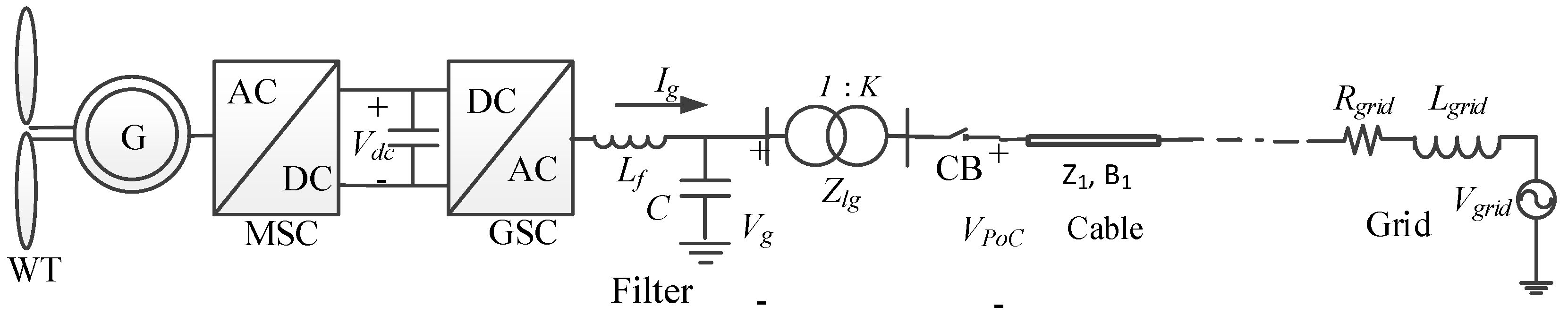
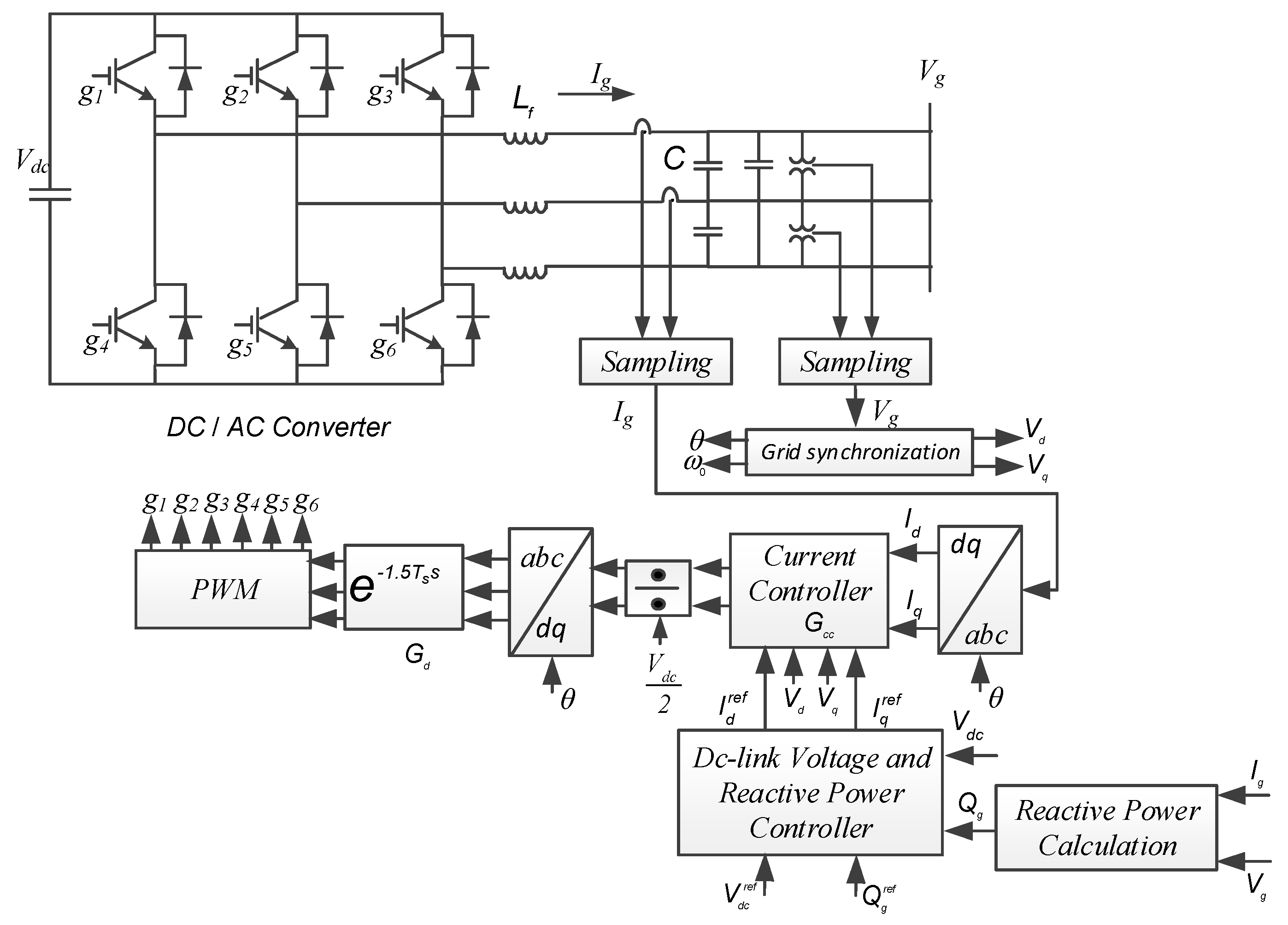
2. Full-Scale Converter-Based Wind Turbines

The full-scale converter configuration, which is shown in Figure 1, is one of the popular configurations for variable speed wind turbines. In this configuration, the grid side converter usually controls the dc-link voltage, and the machine side converter controls the active power [26]. If the small oscillations of the dc-link voltage are neglected, the dynamics of the wind turbine around and above the fundamental frequency can be predicted by modelling of the grid side converter [27]. Therefore, the dynamics of the machine side converter can be neglected in this paper.

Figure 2 shows the grid side converter of a wind turbine with its control in the dq frame. The grid side converter is a voltage source converter, and its control consists of four main parts: grid synchronization, dc-link voltage controller, current controller and pulse width modulation (PWM) [28]. The grid synchronization loop estimates the phase angle of the point-of-connection (PoC) voltage, and this angle is used to transform the signals between the abc frame and the dq frame [29]. The current references (I_d ^ref and I_q ^ref) are generated from the dc-link voltage and reactive power controller. The error of these references is compared to the measured grid currents (I_d and I_q) and fed to proportional integral (PI) controllers (G_cc).

The outputs of the current controllers are fed to the PWM modulator to generate the final switching signals of the insulated-gate bipolar transistors (IGBTs). The time-delay of the PWM and the discrete control can be modelled by using the Padé approximation [30].

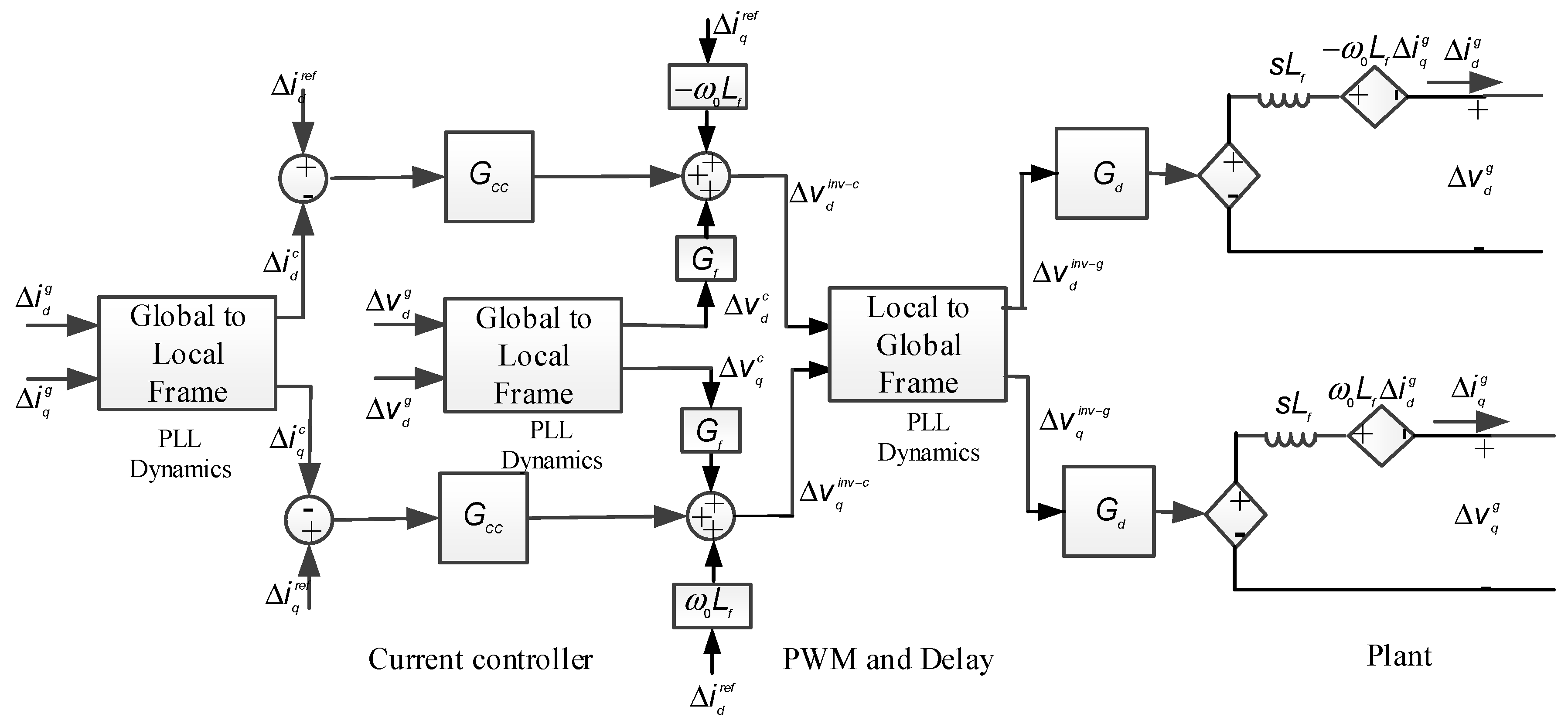
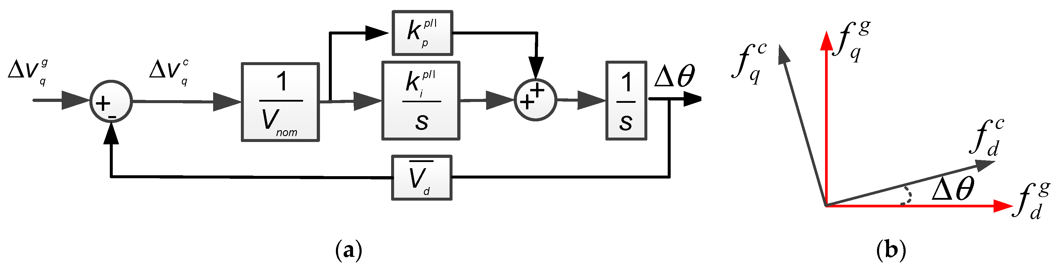
3. Small-Signal Admittance Model in dq-Domain

Figure 3 shows the model of the current controller, the feedforward terms, the PWM modulator and the filter choke of the grid side converter in the dq frame. The measurement delay is very small compared to the PWM delay and can be neglected. An outer dc-link voltage control loop is implemented in the GSC and is responsible to keep the dc-link voltage constant. The bandwidth of this outer control loop is very low compared to the fundamental frequency. This paper focuses on the oscillations around and above the fundamental frequency. Therefore, such low-bandwidth outer loops can be neglected [13]. As it is assumed that the dc-link voltage is constant, the dynamics of the dc-link controller have been neglected. Because of the dynamics of the grid synchronization loop, the dq domain model comprises a fixed global frame and a local controller frame. In the model, the measurement delay is neglected, but the PWM delay (G_d) is included as defined in [30]. The grid voltage is added to the output current controller (G_cc) through a high-pass/low-pass filter (G_f).

According to Figure 3, the small signal output currents and dq output voltage can be obtained by the following matrices:

$$\left[\begin{array}{cc}s{L}_f& -{\omega }_0{L}_f\\ +{\omega }_0{L}_f& s{L}_f\end{array}\right]\left[\begin{array}{c}\Delta i_d^g\\ \Delta i_q^g\end{array}\right]=\left[\begin{array}{cc}{G}_d& 0\\ 0& G_d\end{array}\right]\left[\begin{array}{c}\Delta v_d^{inv-g}\\ \Delta v_q^{inv-g}\end{array}\right]+\left[\begin{array}{cc}-1& 0\\ 0& -1\end{array}\right]\left[\begin{array}{c}\Delta v_d^g\\ \Delta v_q^g\end{array}\right]$$

(1)

$$\left[\begin{array}{c}\Delta v_d^{inv-c}\\ \Delta v_q^{inv-c}\end{array}\right]=\left[\begin{array}{cc}-G_{cc}& 0\\ 0& -G_{cc}\end{array}\right]\left[\begin{array}{c}\Delta i_d^c\\ \Delta i_q^c\end{array}\right]+\left[\begin{array}{cc}{G}_f& 0\\ 0& G_f\end{array}\right]\left[\begin{array}{c}\Delta v_d^c\\ \Delta v_q^c\end{array}\right]$$

(2)

By neglecting the dynamics of the grid synchronization loop, e.g., PLL, the dq frame of the plant and the dq frame of the controller would be the same, i.e.,

$$\left[\begin{array}{c}\Delta i_d^c\\ \Delta i_q^c\end{array}\right]=\left[\begin{array}{c}\Delta i_d^g\\ \Delta i_q^g\end{array}\right]=\left[\begin{array}{c}\Delta i_d^{}\\ \Delta i_q^{}\end{array}\right]\left[\begin{array}{c}\Delta V_d^c\\ \Delta V_q^c\end{array}\right]=\left[\begin{array}{c}\Delta V_d^g\\ \Delta V_q^g\end{array}\right]=\left[\begin{array}{c}\Delta V_d^{}\\ \Delta V_q^{}\end{array}\right]\left[\begin{array}{c}\Delta V_d^{inv-g}\\ \Delta V_q^{inv-g}\end{array}\right]=\left[\begin{array}{c}\Delta V_d^{inv-c}\\ \Delta V_q^{inv-c}\end{array}\right]=\left[\begin{array}{c}\Delta V_d^{inv}\\ \Delta V_q^{inv}\end{array}\right]$$

(3)

By substituting (2) and (3) in (1), the admittance matrix can be obtained as

$$-\left[\begin{array}{c}\Delta i_d^{}\\ \Delta i_q^{}\end{array}\right]=Y_{dq}\left[\begin{array}{c}\Delta v_d^{}\\ \Delta v_q^{}\end{array}\right]\Rightarrow Y_{dq}=-{\left[\begin{array}{cc}s{L}_f+G_d{G}_{cc}& -{\omega }_0{L}_f\\ +{\omega }_0{L}_f& s{L}_f+G_d{G}_{cc}\end{array}\right]}^{-1}\left[\begin{array}{cc}{G}_d{G}_f-1& 0\\ 0& G_d{G}_f-1\end{array}\right]$$

(4)

where the dynamics of the grid synchronization loop are ignored.

For the grid synchronization loop, the synchronous reference frame phase-locked loop (SRF-PLL) can be used and the small signal model is shown in Figure 4.

When small-signal perturbations are added to the V_g voltage, the estimated angle will have a small error (Δθ) between the local (controller) and global (plant) frames because of the PLL dynamics. In Figure 4b, f_dq^c corresponds to the estimated angle and f_dq^g corresponds to the actual angle. Based on Figure 4, the voltage and current in the controller frame and plant frame under small-signal perturbations can be derived as

$$\begin{array}{l}\left[\begin{array}{c}\Delta i_d^c\\ \Delta i_q^c\end{array}\right]=\left[\begin{array}{c}\Delta i_d^g\\ \Delta i_q^g\end{array}\right]+\left[\begin{array}{cc}0& G_{pll}^{}{\overline{I}}_q^{}\\ 0& -G_{pll}^{}{\overline{I}}_d^{}\end{array}\right]\left[\begin{array}{c}\Delta V_d^g\\ \Delta V_q^g\end{array}\right]\left[\begin{array}{c}\Delta V_d^c\\ \Delta V_q^c\end{array}\right]=\left[\begin{array}{c}\Delta V_d^g\\ \Delta V_q^g\end{array}\right]+\left[\begin{array}{cc}0& G_{pll}^{}{\overline{V}}_q^{}\\ 0& -G_{pll}^{}{\overline{V}}_d^{}\end{array}\right]\left[\begin{array}{c}\Delta V_d^g\\ \Delta V_q^g\end{array}\right]\\ \left[\begin{array}{c}\Delta V_d^{inv-g}\\ \Delta V_q^{inv-g}\end{array}\right]=\left[\begin{array}{c}\Delta V_d^{inv-c}\\ \Delta V_q^{inv-c}\end{array}\right]+\left[\begin{array}{cc}0& -G_{pll}^{}{\overline{V}}_q^{inv}\\ 0& G_{pll}^{}{\overline{V}}_d^{inv}\end{array}\right]\left[\begin{array}{c}\Delta V_d^g\\ \Delta V_q^g\end{array}\right]\end{array}$$

(5)

where $\overline{I_d},\overline{I_q},\overline{V_d},\overline{V_q},{\overline{V}}_d^{inv}$ and ${\overline{V}}_q^{inv}$ are the operating point values of the converter. Δθ can be derived as

$$\Delta \theta =G_{pll}\Delta V_q^g=\frac{G_{PI}^{PLL}}{V_{nom}+G_{PI}^{PLL}\overline{V_d}}\Delta V_q^g{G}_{PI}^{PLL}=K_p^{pll}+\frac{K_i^{pll}}{s}$$

(6)

Using (1), (2), (5) and (6) and some simplifications, the small signal admittance matrix can be obtained by

$$\begin{array}{c}{Y}_{dq}=\left[\begin{array}{cc}{y}_{dd}(s)& y_{dq}(s)\\ y_{qd}(s)& y_{qq}(s)\end{array}\right]=-{\left[\begin{array}{c}\Delta V_d^g\\ \Delta V_q^g\end{array}\right]}^{-1}\times \left[\begin{array}{c}\Delta i_d^g\\ \Delta i_q^g\end{array}\right]=-{\left[\begin{array}{cc}s{L}_f+G_{cc}{G}_d& -{\omega }_0{L}_f\\ +{\omega }_0{L}_f& s{L}_f+G_{cc}{G}_d\end{array}\right]}^{-1}\\ \hspace{1em}\times \left[\begin{array}{cc}{G}_f{G}_d-1& -G_{cc}{G}_d{G}_{pll}^{}{\overline{I}}_q^{}+G_f{G}_d{G}_{pll}^{}{\overline{V}}_q^{}-G_{pll}^{}{G}_d{\overline{V}}_q^{inv}\\ 0& G_{cc}{G}_d{G}_{pll}^{}{\overline{I}}_d^{}+G_f{G}_d-G_f{G}_d{G}_{pll}^{}{\overline{V}}_d^{}+G_{pll}^{}{G}_d{\overline{V}}_d^{inv}-1\end{array}\right]\end{array}$$

(7)

4. Equivalent Small-Signal Admittance Model in Sequence Domain

In the previous section, the small-signal admittance model of the converter in the dq domain has been obtained. However, the admittance model can also be obtained in the positive-negative sequence domain [18,20]. The small-signal admittance matrix in the sequence domain can also be written by a 2 × 2 admittance matrix, where its off-diagonal elements show a coupling between the positive and negative components. This coupling is very small and can be neglected [7]. The relationship between the sequence domain admittance definition and dq domain admittance definition [20] can be obtained by the following equation as derived in Appendix A.

$$\left[\begin{array}{cc}{y}_{pp}(s)& y_{pn}(s)\\ y_{np}(s)& y_{nn}(s)\end{array}\right]={\left[\begin{array}{cc}1& 1\\ -j& j\end{array}\right]}^{-1}\left[\begin{array}{cc}{y}_{dd}(s)& y_{dq}(s)\\ y_{qd}(s)& y_{qq}(s)\end{array}\right]\left[\begin{array}{cc}1& 1\\ -j& j\end{array}\right]$$

(8)

The detailed form of Equation (8) is obtained by substituting Equation (7). In this paper, the dq domain admittance is obtained, and then the equivalent sequence admittance is derived based on (8). For the linear stability analysis of the wind power plant in the sequence domain, the coupling terms may be neglected, and the conventional positive impedance is calculated as:

$$Z_p(s)=\frac{1}{y_{pp}(s-j{\omega }_1)}$$

(9)

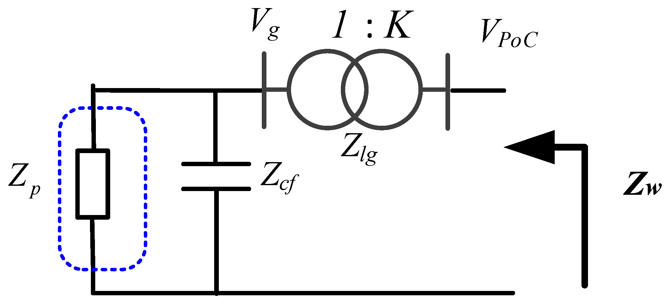
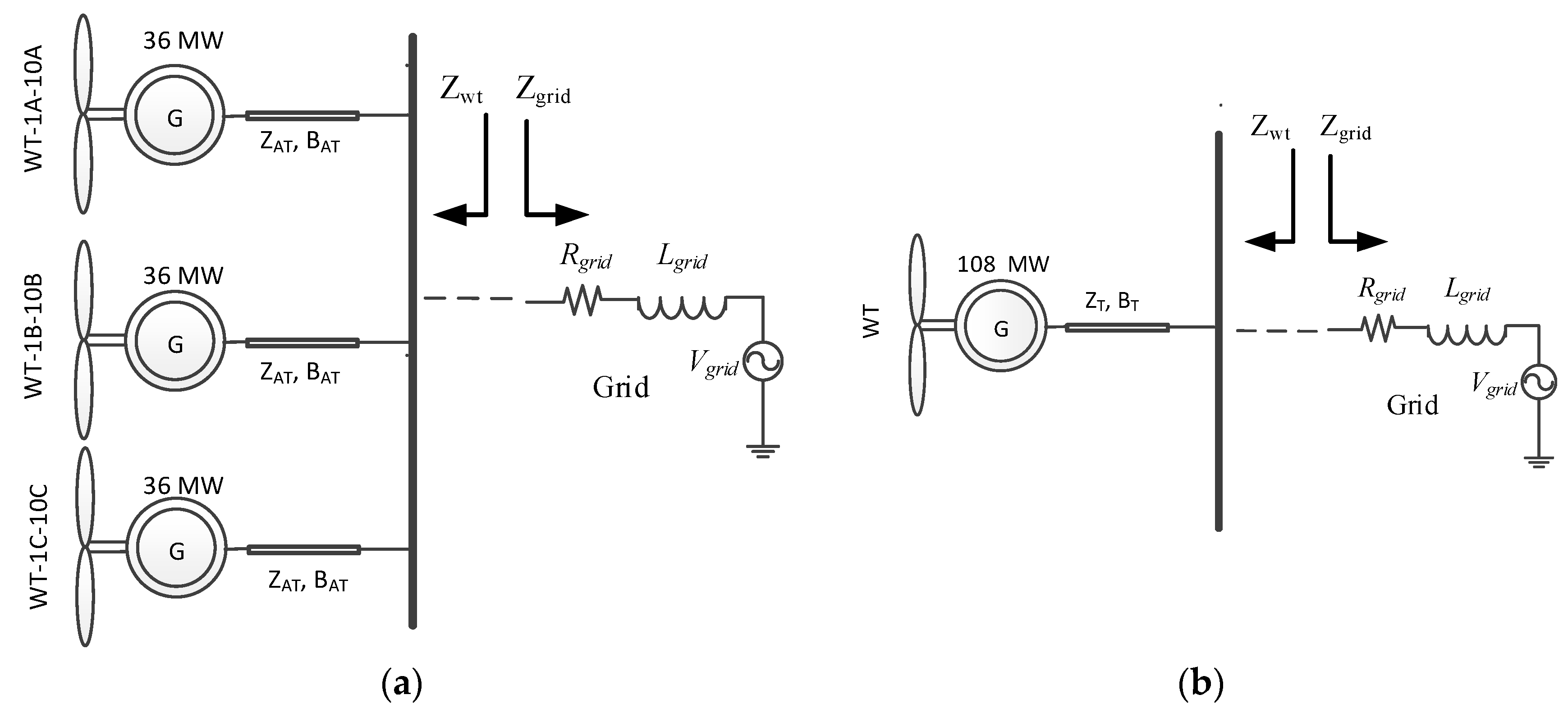
5. Total Wind Turbine Thévenin Impedance

As shown in Figure 5, there is a filter capacitor and a transformer in the output circuit of the wind turbine. Therefore, the total Thévenin impedance of the wind turbine can be equated to

$$Z_W=K_{}^2\left[(\frac{Z_{cf}{Z}_p}{Z_{Cf}+Z_p})+Z_{Lg}\right]=K_{}^2\frac{Z_{Cf}{Z}_p+Z_{Lg}{Z}_p+Z_{Cf}{Z}_{Lg}}{Z_{Cf}+Z_p}$$

(10)

where Z_p is the equivalent small-signal positive impedance of the wind turbine, Z_cf is the filter capacitor impedance, Z_lg is the leakage impedance transformed in the primary side, and K is the transformer voltage ratio. As can be seen, Z_p is in parallel with Z_cf and they are in series with Z_lg. Then this equivalent impedance is transferred to the high-voltage side by the transformer ratio to the power of two (K²).

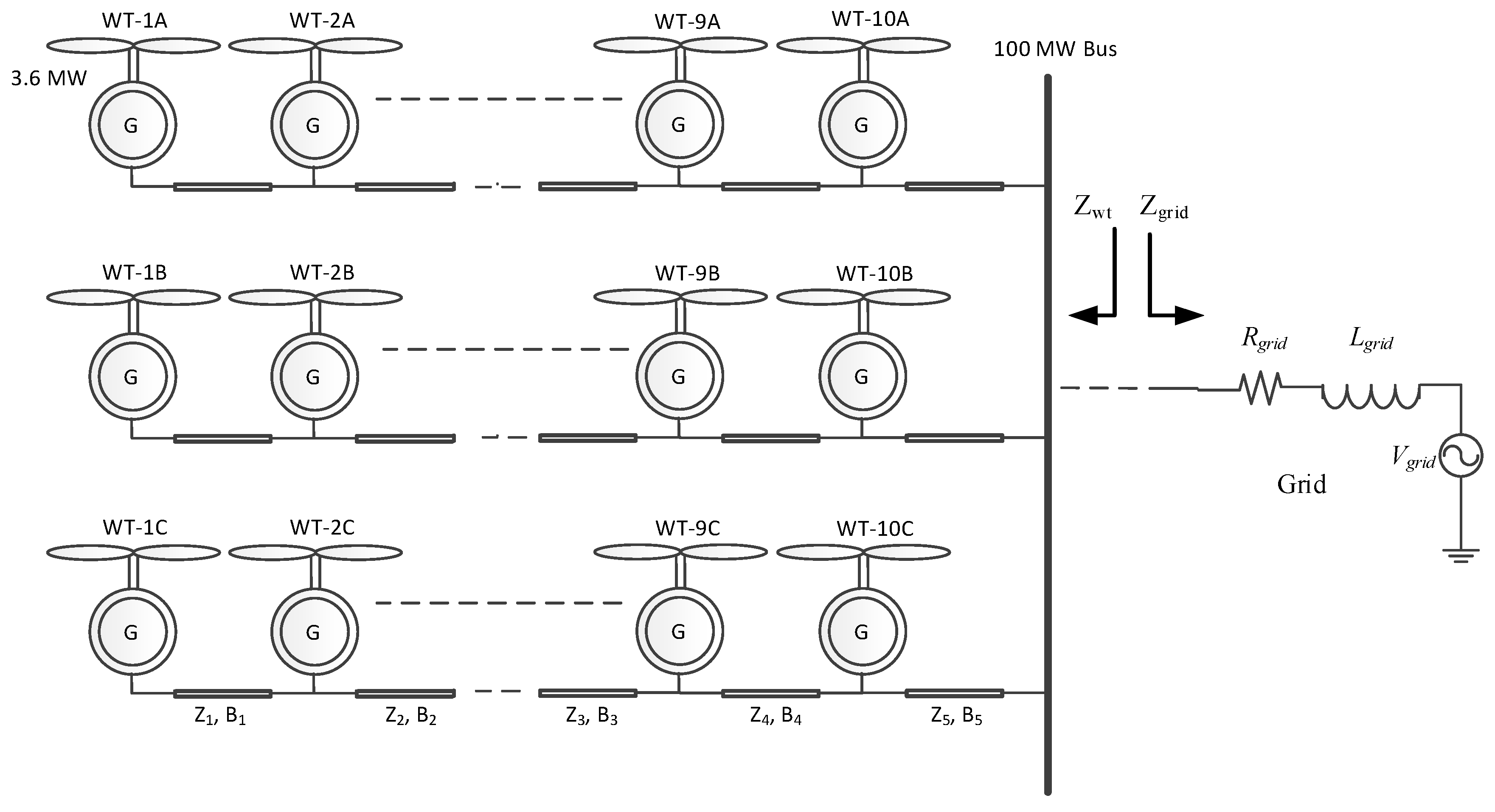
6. Case Study of a Wind Power Plant Connected to a Weak Grid

In order to perform an impedance-based stability analysis, an aggregated model of the wind power plant is required. For example, Figure 6 shows a 108 MW wind power plant with three strings and ten 3.6 MW wind turbines installed on each string. All wind turbines in the wind power plant are assumed to have the same structure. Therefore, the impedance equivalent of the aggregated wind turbines can be obtained based on per-unit values.

If it is assumed that the voltages and currents of the wind turbines are the same, ten 3.6 MW wind turbines of each feeder can be aggregated into one 36 MW wind turbine (see Figure 7), where its equivalent series cable parameter can be obtained [31,32] by

$$Z_{AT}=\frac{{\displaystyle \sum _{m=1}^{10}{m}^2}{Z}_m}{{10}^2}{B}_{AT}={\displaystyle \sum _{m=1}^{10}{B}_m}$$

(11)

Z_AT is the equivalent series impedance, and B_AT is the equivalent shunt susceptance, respectively. Finally, three 36 MW parallel aggregated wind turbines can be aggregated as one 108 MW wind turbine (shown in Figure 7), where its equivalent series parameter can be calculated by

$$Z_T=\frac{Z_{AT}}{3}{B}_T=3B_{AT}$$

(12)

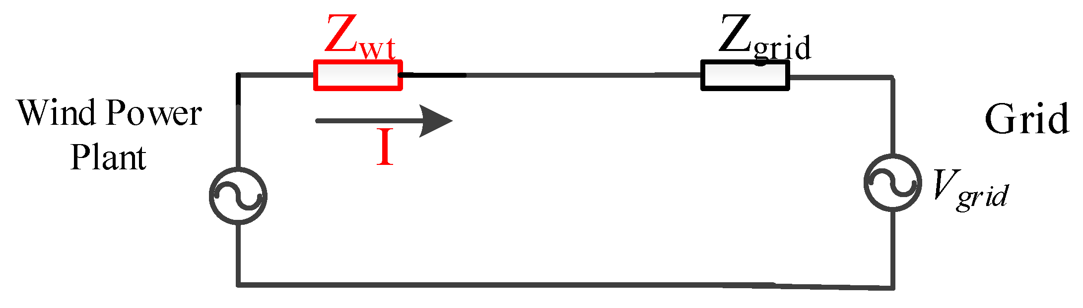
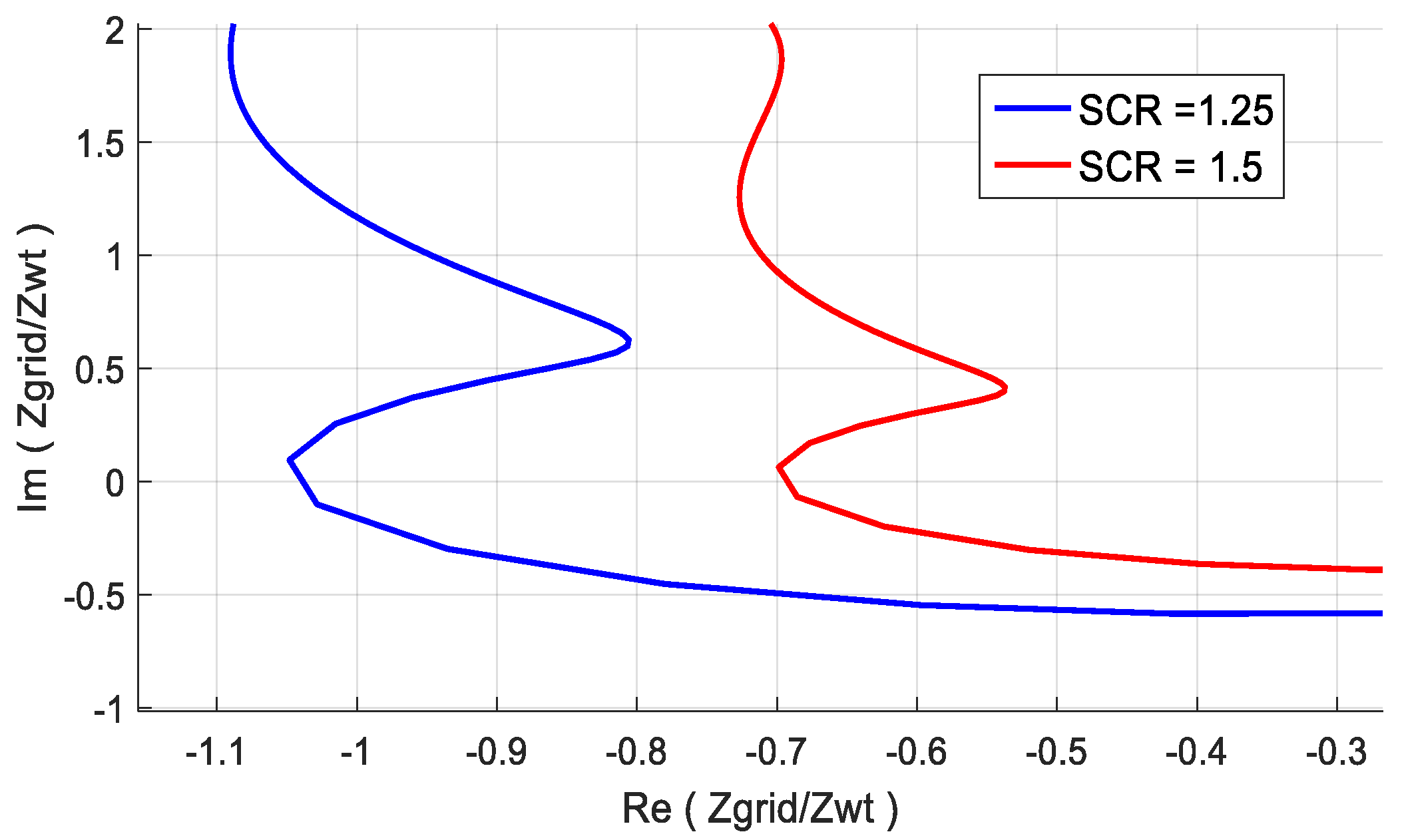
6.1. Stability Analysis

By obtaining the equivalent wind power plant impedance and the equivalent grid impedance, Figure 8 can be used for stability analysis. Based on this figure, the transfer function for the current can be obtained as

$$I(s)=\frac{V_{wt}-V_{grid}}{Z_{wt}+Z_{grid}}=(\frac{V_{wt}-V_{grid}}{Z_{wt}})(\frac{1}{1+Z_{grid}/Z_{wt}})$$

(13)

For the stability analysis, the poles of the system can be obtained by solving the following equation:

$$Z_{wt}+Z_{grid}=0$$

(14)

As the wind power plant is stable when connected to a strong grid, i.e., V_wt/Z_wt has no right-half plane poles, an alternative option for the stability analysis is to assess the Nyquist stability criterion for Z_grid/Z_wt.

A weak grid model is considered here including inductive reactance (X_g), resistance (R), and series capacitive reactance (X_c) for compensation. To illustrate sensitivity to variation in the network, short-circuit level, X_g/R ratio and line series compensation, three scenarios, are studied, all based on a fictitious wind turbine converter controller, the parameters of which are listed in [21]. The wind turbine has been tuned for a strong grid. In Appendix B, all the variables and parameters used in the figures are summarized.

6.1.1. Short Circuit Ratio (SCR) Variations for X_g/R = 20 and X_c/X_g = 0

In this scenario, the SCR is changed from 1.25 to 1.5, X_g/R = 20 and X_c/X_g = 0 (without series compensation). Some poles of the system are shown in

Table 1. Poles for short circuit ratio (SCR) variations for X_g/R = 20 and X_c/X_g = 0.

SCR	P1	P2	P3
1.25	123 + j184	4.61 + j449	−240 + j596
1.5	−117 + j189	−30.6 + j446	−297 + j669

. As it can be seen, there is an unstable pole for SCR = 1.25.

Nyquist criterion-based stability analyses for SCR = 1.25 and SCR = 1.5 are shown in Figure 9. When the SCR = 1.25, there is an encirclement of the point −1, which shows that the system is unstable.

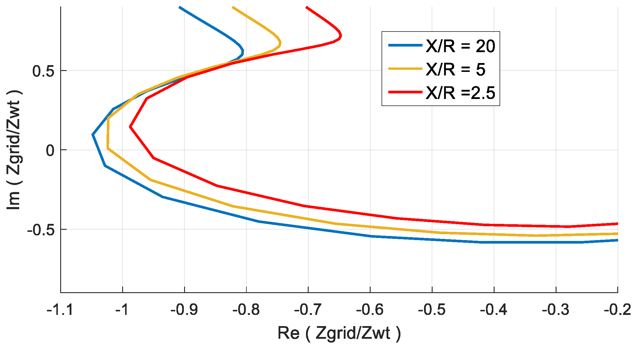
6.1.2. X_g/R variations for SCR = 1.25 and X_c/X_g = 0

In this scenario, X_g/R is decreased from 20 to 5 and to 2.5, when the SCR = 1.25. As it can be seen from the pole analysis in

Table 2. Poles for X_g/R variations for SCR = 1.25 and X_c/X_g = 0.

Xg/R	P1	P2	P3
20	−123 + j184	4.61 + j449	−240 + j596
5	−124 + j189	2.07 + j438	−255 + j596
2.5	−125 + j196	−2.97 + j427	−245 + j596

and the Nyquist analysis in Figure 10, the system becomes more stable by decreasing the X_g/R ratio.

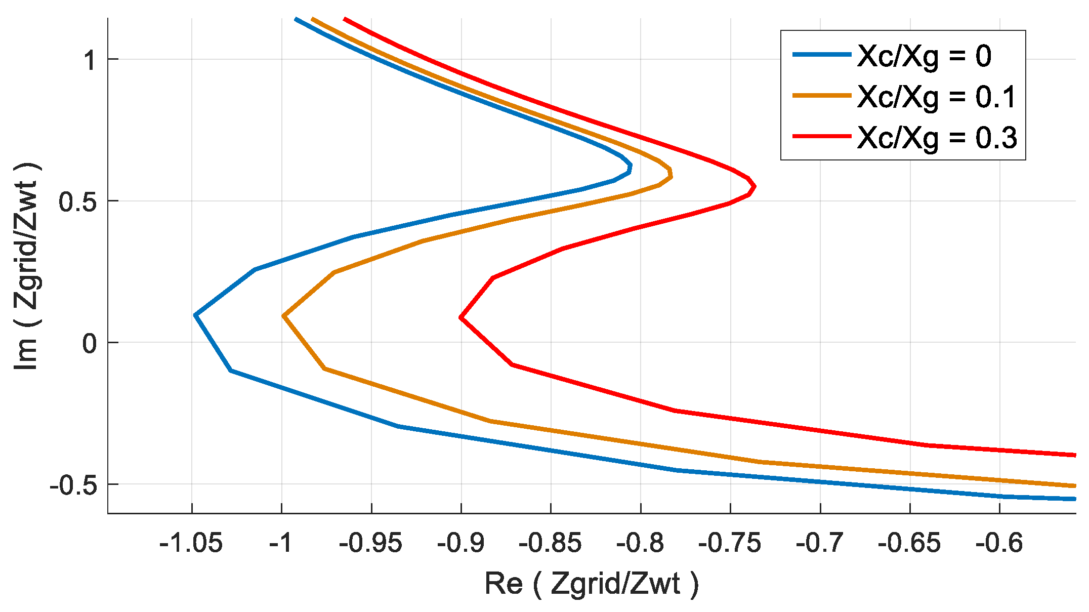
6.1.3. X_c/X_g Variations for SCR = 1.25 and X_g/R = 20

Table 3. Poles for X_c/X_g variations for SCR = 1.25 and X_g/R = 20.

Xc/Xg	P1	P2	P3
0	−123 + j184	4.61 + j449	−240 + j596
0.1	−119 + j182	−0.61 + j449	−239 + j600
0.3	−110 + j175	−11.1 + j450	−237 + j609

and Figure 11 show the corresponding poles and Nyquist criteria under X_c/X_g variations for SCR = 1.25 and X_g/R = 20. It can be seen that the real part of the pole around 70 Hz becomes more negative (more stable) along with more compensation.

In order to validate the frequency-domain analysis, a time-domain simulation was performed for SCR = 1.25, Xg/R = 20 and X_c/X_g = 0. The current injected to the grid and its fast Fourier transform (FFT) are shown in Figure 12. As it can be seen, some oscillations around 73 Hz (459 rad) are increased until the wind turbine goes to trip. This result is matched with the frequency-domain result in Table 1, which indicates there is one unstable mode as 4.61 + j449.

7. Conclusions

This paper presents a unified impedance-based modelling and analysis tool to predict unstable conditions resulting from the interactions between the wind power plant and the weak grid. The proposed approach allows to have advantages of both the dq domain modelling and sequence domain modelling. This enables transmission system operators (TSOs) to do stability analyses of large power systems more efficiently, and it enables wind turbine manufacturers to optimise the controller parameters to increase the stability margin under a weak grid connection. A 108 MW wind power plant has been studied and the short circuit ratio (SCR) of the grid is considered to be 1.25 and 1.5. The poles of the closed-loop system in the frequency-domain are calculated to find the frequency and damping of the oscillatory modes. Nyquist criteria of the open-loop system are plotted to predict easily the stability margin of the wind power plant connected to the weak grid. The results of a simulated wind power plant have shown that a wind power plant which is tuned for a strong grid can become unstable when connected to a weak grid. The proposed method is a valuable tool when adapting and retuning the control system to actual grid conditions.

References

1. Mitra, P.; Zhang, L.; Harnefors, L. Offshore wind integration to a weak grid by VSC-HVDC links using power-synchronization control: A case study. IEEE Trans. Power Del. 2014, 29, 453–461. [Google Scholar] [CrossRef]
2. Pereira, F.J.F.; Rodrigues, J.M.; de Oliveira, K.L.M.; Araujo, D.R.R.P.; de Araujo, L.R. Simulations and analysis of distribution systems with aspects of smart grids using MICQ, RTDS and PSCAD. In Proceedings of the IEEE ISGT Conference, Sao Paulo, Brazil, 15–17 April 2013; pp. 1–8. [Google Scholar]
3. Zhang, Q.; Lu, G.; Zhang, C. Simulated study of the multiple cascade medium-voltage inverter based on PSCAD/EMTDC. In Proceedings of the IEEE ICEMS, Chiba, Japan, 13–16 November 2016; pp. 1–6. [Google Scholar]
4. Pogaku, N.; Prodanovic, M.; Green, T.C. Modeling, analysis and testing of autonomous operation of an inverter-based microgrid. IEEE Trans. Power Electron. 2007, 22, 613–625. [Google Scholar] [CrossRef]
5. Sun, J. Impedance-based stability criterion for grid-connected inverters. IEEE Trans. Power Electron. 2011, 26, 3075–3078. [Google Scholar] [CrossRef]
6. Badrzadeh, B.; Gupta, M.; Singh, N.; Petersson, A.; Max, L.; Høgdahl, M. Power system harmonic analysis in wind power plants—Part I: Study methodology and techniques. In Proceedings of the IEEE IAS, Las Vegas, NV, USA, 7–11 October 2012; pp. 1–11. [Google Scholar]
7. Cespedes, M.; Sun, J. Impedance modeling and analysis of grid connected voltage-source converters. IEEE Trans. Power Electron. 2014, 29, 1254–1261. [Google Scholar] [CrossRef]
8. Bottrell, N.; Prodanovic, M.; Green, T.C. Dynamic stability of a microgrid with an active load. IEEE Trans. Power Electron. 2013, 28, 5107–5119. [Google Scholar] [CrossRef]
9. Singh, A.; Kaviani, A.K.; Mirafzal, B. On dynamic models and stability analysis of three-phase phasor PWM-based CSI for stand-alone applications. IEEE Trans. Ind. Electron. 2015, 62, 2698–2707. [Google Scholar] [CrossRef]
10. Coelho, E.A.A.; Cortizo, P.C.; Garcia, P.F.D. Small-signal stability for parallel-connected inverters in stand-alone AC supply systems. IEEE Trans. Ind. Appl. 2002, 38, 533–542. [Google Scholar] [CrossRef]
11. Kunjumuhammed, L.P.; Pal, B.C.; Oates, C.; Dyke, K.J. The adequacy of the present practice in dynamic aggregated modeling of wind farm systems. IEEE Trans. Sustain. Energy 2017, 8, 23–32. [Google Scholar] [CrossRef]
12. Kwon, J.; Wang, X.; Blaabjerg, F.; Bak, C.L.; Wood, A.R.; Watson, N. Linearized modeling methods of ac-dc converters for an accurate frequency response. IEEE J. Emerg. Sel. Top. Power Electron. 2017, 5, 1526–1541. [Google Scholar] [CrossRef]
13. Wang, X.; Blaabjerg, F. Harmonic stability in power electronic based power systems: Concept, modeling, and analysis. IEEE Trans. Smart Grid 2018, 10, 2858–2870. [Google Scholar] [CrossRef]
14. Wang, Y.; Wang, X.; Blaabjerg, F.; Chen, Z. Small-signal stability analysis of inverter-fed power systems using component connection method. IEEE Trans. Smart Grid 2018, 9, 5301–5310. [Google Scholar] [CrossRef]
15. Gaba, G.; Lefebver, S.; Mukhedkar, D. Comparative analysis and study of the dynamic stability of AC/DC systems. IEEE Trans. Power Syst. 1988, 3, 978–985. [Google Scholar] [CrossRef]
16. Hou, P.; Ebrahimzadeh, E.; Wang, X.; Blaabjerg, F.; Fang, J.; Wang, Y. Harmonic stability analysis of offshore wind farm with CCM. In Proceedings of the IEEE IECON Conference, Beijing, China, 29 October–1 November 2017; pp. 1–6. [Google Scholar]
17. Harnefors, L.; Bongiorno, M.; Lundberg, S. Input-Admittance Calculation and Shaping for Controlled Voltage-Source Converters. IEEE Trans. Ind. Electron. 2007, 54, 3323–3334. [Google Scholar] [CrossRef]
18. Shah, S.; Parsa, L. Impedance Modeling of Three-Phase Voltage Source Converters in DQ, Sequence, and Phasor Domains. IEEE Trans. Energy Convers. 2017, 32, 1139–1150. [Google Scholar] [CrossRef]
19. Holmes, D.G.; Lipo, T.A. Pulse Width Modulation for Power Converters: Principles and Practice; Wiley: Piscataway, NJ, USA, 2003. [Google Scholar]
20. Rygg, A.; Molinas, M.; Zhang, C.; Cai, X. A modified sequence-domain impedance definition and its equivalence to the dq-domain impedance definition for the stability analysis of AC power electronic systems. IEEE Trans. Emerg. Sel. Top. Power Electron. 2016, 4, 1383–1396. [Google Scholar] [CrossRef]
21. Ebrahimzadeh, E.; Blaabjerg, F.; Wang, X.; Bak, C.L.; Lund, T.; Andersen, G.K.; Suárez, C.G.; Berg, J. Small signal modeling of wind farms. In Proceedings of the IEEE ECCE Conference, Cincinnati, OH, USA, 1–5 October 2017; pp. 1–7. [Google Scholar]
22. Wen, B.; Boroyevich, D.; Burgos, R.; Mattavelli, P.; Shen, Z. Small signal stability analysis of three-phase AC systems in the presence of constant power loads based on measured d−q frame impedances. IEEE Trans. Power Electron. 2015, 30, 5952–5963. [Google Scholar] [CrossRef]
23. Wen, B.; Boroyevich, D.; Burgos, R.; Mattavelli, P.; Shen, Z. Analysis of D-Q small-signal impedance of grid-tied inverters. IEEE Trans. Power Electron. 2016, 31, 675–687. [Google Scholar] [CrossRef]
24. Kunjumuhammed, L.P.; Pal, B.C.; Oates, C.; Dyke, K.J. Electrical oscillations in wind farm systems: Analysis and insight based on detailed modeling. IEEE Trans. Sustain. Energy 2016, 7, 51–62. [Google Scholar] [CrossRef]
25. Kwon, J.; Wang, X.; Blaabjerg, F.; Bak, C.L.; Wood, A.R.; Watson, N. Harmonic instability analysis of a single-phase grid-connected converter using a harmonic state-space modeling method. IEEE Trans. Ind. Appl. 2016, 52, 4188–4200. [Google Scholar] [CrossRef]
26. Zhang, Z.; Wang, F.; Wang, J.; Rodríguez, J.; Kennel, R. Nonlinear direct control for three-level NPC back-to-back converter PMSG wind turbine systems: Experimental assessment with FPGA. IEEE Trans. Ind. Inf. 2017, 13, 1172–1183. [Google Scholar] [CrossRef]
27. Ebrahimzadeh, E.; Blaabjerg, F.; Wang, X.; Bak, C.L. Bus participation factor analysis for harmonic instability in power electronics based power systems. IEEE Trans. Power Electron. 2018, 33, 10341–10351. [Google Scholar] [CrossRef]
28. Xing, P.; Fu, L.; Wang, G.; Wang, Y.; Zhang, Y. A compositive control method of low-voltage ride through for PMSG-based wind turbine generator system. IET Gen. Transm. Distrib. 2018, 12, 117–125. [Google Scholar] [CrossRef]
29. Yu, L.; Li, R.; Xu, L. Distributed PLL-based control of offshore wind turbine connected with diode-rectifier based HVDC systems. IEEE Trans. Power Del. 2018, 33, 1328–1336. [Google Scholar] [CrossRef]
30. Wang, J.; Yan, J.D.; Jiang, L.; Zou, J. Delay-dependent stability of single-loop controlled grid-connected inverters with LCL filters. IEEE Trans. Power Electron. 2016, 31, 743–757. [Google Scholar] [CrossRef]
31. Ebrahimzadeh, E. Electrical Oscillations in Wind Power Plants: Modeling, Control, and Mitigation. Ph.D. Thesis, Aalborg University, Aalborg, Denmark, 2018. [Google Scholar]
32. Muljadi, E.; Pasupulati, S.; Ellis, A.; Kosterov, D. Method of equivalencing for a large wind power plant with multiple turbine representation. In Proceedings of the IEEE Power and Energy Society General Meeting, Pittsburgh, PA, USA, 20–24 July 2008; pp. 1–9. [Google Scholar]
Figure 1. Simplified representation of full-scale converter-based wind turbine connected to the network.
Applsci 09 04695 g001
Figure 2. Grid side converter and its control, as typically used in wind turbines.
Applsci 09 04695 g002
Figure 3. Dq small signal model of the current controller, PLL and the filter inductance (Lf).
Applsci 09 04695 g003
Figure 4. Synchronous reference frame phase-locked loop (SRF-PLL), (a) small signal model of PLL, (b) controller (fdqc) and system (fdqg) frames under small-signal perturbations because of the PLL dynamics.
Applsci 09 04695 g004
Figure 5. Simplified wind turbine (WT) system model, Zp = equivalent small-signal positive impedance, Zcf = filter capacitor impedance, Zlg = leakage impedance.
Applsci 09 04695 g005
Figure 6. A 108 MW wind power plant, including three 36 MW strings.
Applsci 09 04695 g006
Figure 7. Aggregated model of the 108 MW wind power plant shown in Figure 8, (a) aggregated model on each string as one 36 MW wind turbine, (b) aggregated model of three strings into one 108 MW wind turbine.
Applsci 09 04695 g007
Figure 8. Aggregated wind power plant model connected to weak grid.
Applsci 09 04695 g008
Figure 9. Nyquist criteria under SCR variations for Xg/R = 20 and Xc/Xg = 0.
Applsci 09 04695 g009
Figure 10. Nyquist criteria under Xg/R variations for SCR = 1.25 and Xc/Xg = 0.
Applsci 09 04695 g010
Figure 11. Nyquist criteria under Xc/Xg variations for SCR = 1.25 and X/R = 206.1.4. Time-domain simulation result.
Applsci 09 04695 g011
Figure 12. Time-domain simulation for SCR = 1.25, Xg/R = 20 and Xc/Xg = 0 (an unstable case), (a) current, (b) fast Fourier transform (FFT) of the current before trip.
Applsci 09 04695 g012aApplsci 09 04695 g012b