Detection and Classification of Advanced Persistent Threats and Attacks Using the Support Vector Machine

Abstract

Traditional network attack and hacking models are constantly evolving to keep pace with the rapid development of network technology. Advanced persistent threat (APT), usually organized by a hacker group, is a complex and targeted attack method. A long period of strategic planning and information search usually precedes an attack on a specific goal. Focus is on a targeted object and customized specific methods are used to launch the attack and obtain confidential information. This study offers an attack detection system that enables early discovery of the APT attack. The system uses the NSL-KDD database for attack detection and verification. The main method uses principal component analysis (PCA) for feature sampling and the enhancement of detection efficiency. The advantages and disadvantages of using the classifiers are then compared to detect the dataset, the classifier supports the vector machine, naive Bayes classification, the decision tree and neural networks. Results of the experiments show the support vector machine (SVM) to have the highest recognition rate, reaching 97.22% (for the trained subdata A). The purpose of this study was to establish an APT early warning model mechanism, that could be used to reduce the impact and influence of APT attacks.

1. Introduction

The recent boom in the development of Internet technology has caused a similar boom in hacker attack methods which is being constantly updated. Industry, as well as government, now face more serious threats to information security. The threat to information from advanced persistent threat (APT) is much greater than that from independent hackers and poses an enormous challenge to network information security systems [1,2]. Among the important characteristics of APT is that it is advanced and intrusion is at a very high level. It also has strong shielding ability and the attack path is often indiscernible and this makes it more difficult for traditional methods to detect and put up a defense. It is also persistent, the attack is continuous and of long duration, this also makes it difficult for single, point based, detection techniques to handle. Although APT’s carrier exists in big data, it brings a series of difficulties to APT detection and protection, but it can also use big data to test and respond to APT. If there is comprehensive information data at all levels and stages, and any interactive behavior is detected, different data can be used to find different stages for APT analysis. APT is a major attack model that goes on for a long time, involves a large amount of data traffic, and is multi-faceted. This mode of attack presents major hurdles to which traditional single-point feature matching detection can hardly put up serious and effective resistance.

In 2013, Mandiant, now part of the FireEye US Information Network Security group, classified an APT attack as being cyclic and having five stages. The first is an initial invasion, mainly using email as the medium. The second stage is the establishment of a foothold, and malicious programs are used to take hold of the target system. The third stage involves gaining administrator privileges and cracking the password to obtain control and user authority. An internal investigation and parallel diffusion comprise the fourth stage where the main task is a search for other nearby servers and the acquisition of internal related information. The final stage is continuous monitoring and control of the server, and the theft and export of data [3]. The APT attack threat is getting more serious, its evolution speed is beyond imagination, while its form has become more diversified. The techniques APT has adopted for different targets and objects have also changed. The common methods now used for APT attacks are watering hole, spear phishing, and SQL injection attacks, and some others [4,5].

The detection schemes for APT attacks include sandbox detection, network anomaly detection, and full traffic detection. However, the existing APT attack detection methods have lower accuracy and require a large number of labeled samples. Heba et al. evaluated the NSL-KDD dataset and proposed an anomaly intrusion detection system based on SVM, where PCA is applied for feature selection. They examined the effectiveness of the intrusion detection system by conducting several experiments on the NSL-KDD dataset [6]. Liu et al. proposed a deep intrusion-based network intrusion detection model (DBN-SVDD) [7]. This method uses DBN (deep belief net) for structural dimensionality reduction to improve detection efficiency and it uses SVDD (support vector data description) to identify and detect data sets. The experimental results of the NSL-KDD dataset using various algorithms show that the detection rate of the method can reach 93.71%. There is no need to mark a large number of samples, it can process high-dimensional data, detection of an APT attack is effective and there is no need for supervision.

The frequency of automatic attacks on networks has increased enormously as has the speed and variety of malware employed. The provision of effective analysis processing on big data networks is very important. Incidentally, the processing capacity of the attack data almost always exceeds the capabilities of personal computers. Providers use many different network intrusion detection system (NIDS) devices [8] that are available on the market. Most use the sniffer method to give real-time packet monitoring on the network and compare suspicious packets with others used in previous attacks. When a suspected intrusion is found, these defense systems can launch an immediate warning. There is so far no indication of which algorithm, of the many, used by any hardware device gives the best rate of APT data detection. Currently, there are three common types of APT attack detection: sandbox, abnormal network, and full-flow detection. All have shortcomings and low accuracy and require a large number of labeled samples. Most focus on one stage of the APT attack, and such single detection methods cannot monitor the life cycle of an APT attack at every stage. It is necessary to study the attack data and establish an integrated security detection architecture for the APT that can deal with the complexities of the attack. APT security detection architecture uses stratified thinking to cover all the stages of an APT attack, including preparation, intrusion, infiltration, and harvest stages. It is an in-depth detection system that covers multiple information sources and network protocols. The attackers may be lucky enough to bypass one of the detection stages, but it is very difficult to avoid detection completely.

In the new era of big data, the huge volume of data now spread around the entire globe has brought with it new security challenges far greater than encountered ever before. There is a corresponding and parallel relationship between the space of reality, or real space and data space. Any activity, interaction, and behavior, especially as news, in real space has a corresponding relationship in data space. Information about the vast numbers of worldwide enterprises and their data, about billions of individuals and even objects, cloud computing and the Internet of Things are all carriers that generate big data. There is no doubt about the existence of big data, but it has also become the main carrier of cyber-attacks.

Many experiments have been carried out using the KDD 99 database [9], which has been the most commonly used in past studies. This data is based on a database established by DARPA in 1999. DARPA collected the data of three weeks of normal data flow and two weeks of an anomaly attack. This work was done at the Lincoln Labs of the Massachusetts Institute of Technology (MIT) and there are 494,021 records in the database data training set, and 311,029 records in the test set. There are a total of 41 features and 5 types of large tags (normal, dos, r2l, u2l, probe) [10,11]. The inherent flaws in the KDD 99 data set have been revealed by various statistical analyses, where many studies found flaws that affect the precision of the intrusion detection system (IDS) modeling. Tavallaee et al. [11] questioned the KDD 99 data, and further modified the data sample. He introduced the NSL-KDD database, which is more discriminative and allows better intrusion detection.

The NSL-KDD data set was used in this study. It is suitable for the study and evaluation of network intrusion detection systems [11]. Its predecessor was an improved version of KDD 99 [9], which had redundant data removed, and overcame the classifier recurring records problem that tended to affect learning performance. In addition, the ratio of normal to anomalous data is properly selected, the test and training data volumes are more reasonable, and it is generally more suitable for the accurate evaluation of different machine learning techniques. Big data has become the foundation of science and clarification, structuration, standardization, dimensionality reduction, and visualization. Dimensionality reduction algorithms map the original multidimensional data to low- dimensional data and describe the main features of the original with less data. Common methods currently used can be linear or non-linear. The most frequently used non-linear dimensionality reduction methods are locally linear embedding (LLE) and local tangent space alignment (LTSA) [12]. However, the computational complexity of non-linearity is high, and in this study, it was necessary to process rapidly, even immediately, and so linear dimensionality reduction was used. The focus of this study was on the exploration of linear principal component analysis (PCA) [13] as the main axis. The three important characteristics of PCA are: (1) it is the best linear scheme, in terms of mean square error, for the compression and reconstruction of a set of high-dimensional vectors into lower-dimensional vectors; (2) it can directly calculate model parameters from data, such as sample covariance; (3) compression and decompression are simple processes for the execution of model parameters. In line with a method proposed by Revathi et al. [14], the NSL-KDD data set was used for network intrusion detection. The data set has 41 attributes, some of which may not be necessary and others unrelated. When the data set is very large dimensional problems may arise. To reduce the dimensions, we used PCA, a dimensional and multivariate analysis technique primarily used for data compression, image processing, pattern recognition, and time series prediction [15,16].

APT attack detection technology has also been combined with data mining techniques [17,18]. The aim being to carry out data integration and classification using frequently encountered pattern sets and association rules to detect and gain early warning of an APT attack. Classification is divided into categories that have been established using the test data. During the data mining process, attack detection technology becomes a classification issue that determines the category and feature sets. Each audit record is classified as one of two types: normal behavior or attack behavior. In APT attack detection, correlation analysis can be used to find the relationship between the various kinds of attack behavior. This correlation is used to classify the data and for the detection of attacks. The most influential classification algorithms used in data mining are the Iterative Dichotomizer 3 (ID3), C4.5 [19,20], the native Bayes classifier, based on the posterior attitude that uses the Bayes theorem and the backpropagation of the Bayesian and neural networks. If prediction accuracy, calculation speed, robustness, and interpretability are used to evaluate the classification algorithms, it is found that each different method has advantages and disadvantages. No method has so far been found that is superior to the others for all data. They are selected according to the type of data and the application field.

In this study the (NSL-KDD) data set provided by knowledge discovery and data mining (KDD) CUP [11] was used. Although the NSL-KDD dataset data is old, its network communication protocol and attack behavior patterns remain unchanged. The dimension was reduced using PCA to enhance the efficiency of detection. The relevant classification method was then used for the data set experiments and to establish models for the training data (using the training algorithm) to analyze and classify the APT attack packets. The test data were loaded using the training model to obtain the performance indicator. The model was then used to establish the APT attack detection system. Detection and defense covered all stages of the APT attack to achieve the best result.

2. Methods

2.1. Materials and Experimental Setup

The analysis of APT network attack packets is not new technology, but it has become an essential part of network administrators and information security and is used to analyze regular activities. In the past, it usually applied to the analysis of network behavior or debugging of the network environment. In the current network milieu, where information security incidents are frequent, this investigation has become regular and essential. Side recording of network packets from a target host can provide information about events that enables even more information to be obtained through analysis. Therefore, while facing current popular APT attacks hidden behind communication behavior, and even in the communication content, it is possible to obtain key information by using network packet analysis technology. In this study, a comparison has been made between the correct rate of APT network attack detection using the NSL-KDD data sets and PCA dimensionality reduction technology and four machine learning classification algorithms: SVM, naive Bayes, decision tree, and the multi-layer perceptron neural network (MLP). Most relevant work has been done using the “WEKA Spreadsheet to ARFF” service to convert the NSL-KDD data set format from files with the csv extension to ARFF extension format (including “training data set (KDDTrain+)” and “test data set (KDDTest+)” (https://github.com/jmnwong/NSL-KDD-Dataset) is the reference URL. Because the data has different ranges, preprocessing needed to be done to round up all the features. Two type classifiers were used, normal, and anomaly. The PCA algorithm was then used to reduce the size of the classified data set. Finally, the pre-processed training and test data sets were grouped and tested, and experiments with the four classification algorithms were carried out. These were SVM [21,22,23], naive Bayes [24], decision tree [25], and MLP and they were used to train and test the data and compare and analyze the results. Each record had data with 41 different feature attributes presenting the content of the network packets. There were four categories of anomalous attack DoS, Probe, R2L, and U2R and the definitions are shown in

Table 1. Four classified categories of anomalous attack

Type of Anomaly	Definition	Related Features
DoS	Distributed denial-of-service (DoS) exhausts the target resources, making it impossible to process legitimate requests.	Original bit Percentage of error packets
Probe	The goal of surveillance and other probe attacks is to gather related information about remote victims.	Continuous connection time Original bit
R2L	Unauthorized remote machine connection, the attacker invades the remote machine and gains local access to the target system.	Internet rights Continuous connection time Services requested Level features of the host Number of failed login attempts
U2R	Unauthorized access as a local user (admin/root) administrative privileges. The attacker logs into the target system using a regular account and attempts to obtain administrator and root privileges by exploiting certain system vulnerabilities.	Number of file creations Usage times of shell

.

2.2. Method of Signal Dimension Reduction

PCA is a statistical technique that transforms a set of possible correlation variables to a set of linearly uncorrelated variables by orthogonal transformation. The transformed set of variables is the principal component. A set of related features in high-dimensional data is converted to a smaller subset and named as principal component. High-dimensional $n$ data can be transformed to low-order $k$ dimension data ($n>k$). PCA does this transformation by finding a $k$ feature vector, and projecting the $n$ dimension data onto that feature vector to minimize the overall projection error. PCA can preserve around 0.9 variance of the original data set and significantly reduce the number of features as well as the dimensions. The original high-dimensional data set is projected onto a smaller subspace while preserving most of the information contained in the original data set. Assuming $\left\{x_t\right\}$, and $t=1,2,\dots ,N$, the random dimension $n$ with the mean ($\mu$) inputs the data recording its definition as (1)

$$\mu =\frac{1}{N}{\displaystyle \sum _{t=1}^N{x}_t}$$

(1)

The definition f the covariance matrix of $x_t$ is (2):

$$C=\frac{1}{N}{\displaystyle \sum _{t=1}^N\left(x_t-\mu \right){\left(x_t-\mu \right)}^T}$$

(2)

PCA solves the eigenvalues problem of Covariance matrix $C$

$$CC{v}_i={\lambda }_i{v}_i$$

(3)

In Equation (3), ${\lambda }_i$ is the eigenvalue and $v_i$ is the corresponding eigenvector.

To represent the data record with a low-dimensional vector, only $m$ pieces of eigenvector (named as the principal direction) are needed, corresponding to $m$ pieces of the largest eigenvalue ($m<n$), and the variance of the projection of the input data in the principal direction is greater than the variance in any other direction. Hence parameter $v$ is the approximate precision of the $m$ pieces of the largest eigenvector, so the following relationship (4) is obtained

$$\frac{{\displaystyle \sum _{i=1}^m{\lambda }_i}}{{\displaystyle \sum _{i=1}^n{\lambda }_i}}\ge v$$

(4)

The purpose of PCA is to maximize internal information and increase calculation speed after dimension reduction, and to evaluate the importance of the direction by the size of the data variance in the projection direction.

3. Classifier

3.1. Support Vector Machine

SVM technology was devised for handling data in space. A hyperplane in the space is found which separates the data into two different groups. Suppose we have a bunch of points and the rendezvous point is expressed as (5)

$$\left\{x_i,y_i\right\},i=1,\dots ,n\mathrm{and}{x}_i\in R^d,y_i\in \left\{+1,-1\right\}$$

(5)

An attempt is made to find a straight line $f(x)=w^{T}x-b$ that allows all the $y_i=-1$ points to fall on the $f(x)<0$ side, and all the $y_i=+1$ to fall on the $f(x)>0$ side. Therefore, it is possible to distinguish to which side a point belongs by the sign (+ or −) of $f(x)$. This spatial plane is called the separating hyperplane, and the greatest distance from the margin is called the optimal separating hyperplane (OSH). Solving OSH is equivalent to finding the support hyperplane with the farthest distance.

The support hyperplane is defined as in (6)

$$\begin{array}{l}{w}^{T}x=b+\xi \\ w^{T}x=b-\xi \end{array}$$

(6)

The margin between the two separating hyperplanes is naturally double $d$. Where the margin = 2d = 2/‖w‖, the smaller the ‖w‖, the larger the margin. Knowing that the distance between the support hyperplane and the optimal separating hyperplane is within ±1, so the constraint conditions are written as in Equations (7) and (8)

$$y_i\left(w^T{x}_i-b\right)-1\ge 0$$

(7)

The Lagrange multiplier is then used for transformation to a quadratic Equation (8) and to find $w$, $b$, and $\alpha$ that allows L to be a minimum, as in Equation (8)

$$L\left(w,b,\alpha \right)=\frac{1}{2}{\Vert w\Vert }^2-{\displaystyle \sum _{i=1}^N{\alpha }_i\left[y_i\left(w^T{x}_i-b\right)-1\right]}$$

(8)

To solve the minimum value $L$, find the partial differential of $w$ and $b$ respectively to get (9)

$$L_D={\displaystyle \sum _{i=1}^N{\alpha }_i-\frac{1}{2}{\displaystyle \sum _{i,j}{\alpha }_i{\alpha }_j{y}_i{y}_j{x}_i^T{x}_j}}$$

(9)

However, the solution for nonlinear data is to project the data to a space of higher dimension or a feature space. The mapping of x to the feature space through φ, is shown in (10)

$$x_i^T{x}_j\to \phi {(x_i)}^T\phi (x_j)$$

(10)

However, the mapping function φ is very complicated and it is not easy to obtain the value, but its inner product type may become very simple. Take the radial based function (RBF) as an example. Although RBF is a complex function, it can be changed to an inner product and simplified as shown in (11)

$$k\left(x_i,x_j\right)=\phi {(x_i)}^T\phi (x_j)=\exp \left(\frac{-{\Vert x_i-x_j\Vert }^2}{2\sigma }\right)$$

(11)

The function obtained by the mapping function from the inner product is the SVM kernel.

3.2. Naive Bayes

Naive Bayes predicts the results of classification according to the Bayesian theorem. It is mainly used to calculate the data of unknown categories and the probability of its belonging to a category. Bayesian classification attains minimum error by the analysis of probability statistics, using known category attribute probability values and their pre-probability values, to calculate the probability of a new case in each category. The probability of each category is compared and the case will be classified as the category with the greatest probability. Assume that event $c_1,c_2,\dots ,c_n$ is in $n$ category data collection sample space, an observe quantity $X={\left[x_1,x_2,\dots ,x_r\right]}^T$ is then given which has an $r$ features parameter. According to the Bayesian theorem, the classification $c_i$ belongs to the observe quantity $X$, and the error probability of classification can be expected to be minimized. The following Equation (12) can be obtained from the Bayesian theorem.

$$P\left(C_i|X\right)=\frac{P\left(C_i\right)P\left(X|C_i\right)}{P\left(X\right)}$$

(12)

In Equation (12), $P\left(C_i\right)$ is the pre-probability, and represents the probability of the $C_i$ category. $P\left(X\right)$ is a constant, $P\left(X|C_i\right)$ is the probability of observe quantity $X$ and appears in the $C_i$ category. $P\left(C_i|X\right)$ is the post-probability and reference used to judge the $C_i$ category, to which the observe quantity $X$ belongs, the judgment Equation is (13)

$$X\in C_i\mathrm{if}P\left(C_i|X\right)>P\left(C_j|X\right)\mathrm{for}i\le j\le ni\ne j$$

(13)

To judge to which category a certain feature $X$ belongs, it is only necessary to estimate the similarity rate between category $C_i$ and category $C_j$, where the similarity rate $R$ is given by Equation (14)

$$R=\frac{P\left(C_i|X\right)}{P\left(C_j|X\right)}=\frac{P\left(C_i\right)P\left(X|C_i\right)}{P\left(C_j\right)P\left(X|C_j\right)}$$

(14)

If $R>1$, then $X$ is biased towards category $C_i$; on the other hand, if $R<1$, $X$ is more biased towards category $C_j$.

3.3. Decision Tree

The decision tree algorithm classifies data to achieve the purpose of detection. The decision tree is formed from the training set data. If the tree cannot offer a correct classification of all the objects, then some exceptions are selected and added to the training set. This is repeated until a correct decision set has been formed. J48 is a decision tree C4.5 algorithm developed for the generation of decision trees as an extension of the ID3 algorithm previously developed by Quinlan [17,18]. The decision tree generated by the C4.5 algorithm can be used for classification purposes. Information gain is an attribute selection method of information theory, the formal definition is, $I(X)$ and is the information before testing and after the training set has been classified. $E{(\mathrm{A}}_{\mathrm{k}},\mathrm{X})$ is the information after testing, which represents the information in each subset after the training set has been tested by the attribute A_k. Its Equation (15) is shown below

$$\begin{array}{l}\mathrm{Gain}(A_k,X)=I(X)-E(A_k,X)\\ E(A_k,X)={\displaystyle \sum _{i=1}^n\frac{\left|X_i\right|}{\left|X\right|}}I(X_i)\end{array}$$

(15)

In the equation, $X$ is the finite set of examples, $A_k=\left\{A_{1,\dots ,}{A}_p\right\}:$ a set of attributes. The decision tree generated by Equation (15) is gradually trimmed to form a complete decision tree, and further trimmed to give easy-to-understand rules. The advantage of using the C4.5 algorithm is that it can be pruned during the tree construction process. Discretization processing of the continuous attributes allows the processing of incomplete data. The generated classification rules are easy to understand, and have high accuracy. The disadvantage is that the data set needs to be scanned and sorted many times during the process of building the tree. This inefficiency increases computer calculation time. The J48 algorithm has two important parameters, C and M. C is the confidence level used to define the confidence intervals. The value of the confidence factor is based on the trimmed parameter after the decision tree has been established. The smaller the value, the more the tree has been trimmed. The M parameter is the smallest sample number in two of the most popular branches.

3.4. Multilayer Perceptron

Multilayer perceptron (MLP) is a back-propagation neural network with high learning accuracy and fast recall. It can handle complex sample discrimination and highly nonlinear function synthesis problems where the output values can be suspended values. It is a popular neural network that has a wide range of applications that include: sample identification, bifurcation problems, function simulation, prediction, system control, noise filtering, data compression, etc.

MLP is a back-propagating supervised learning algorithm, through $f(·):R^m\to R^o$, m is the dimension at input and $o$ is the dimension at output. By inputting the feature $X=x_1,x_2,\dots x_m$ and the target value Y, this algorithm can classify the data using nonlinear approximation or perform regression. MLP can have many nonlinear layers inserted between the input and output layers.

The stochastic gradient descent (SGD) method is used in MLP training. SGD uses the gradient of the loss function, relative to the parameter that needs to be adaptive for updating, see Equation (16), where $\eta$ is the learning rate in the control parameter space search step, and Loss is the loss function used by the network.

$$w\leftarrow w-\eta \left(\alpha \frac{\partial R\left(w\right)}{\partial w}+\frac{\partial \mathrm{Loss}}{\partial w}\right)$$

(16)

If a training sample set $\left(x_1,y_1\right),\left(x_2,y_2\right),\dots \dots ,\left(x_n,y_n\right)$ is given, where $x_i\in R^n$ with $y_i\in \left\{0,1\right\}$, then the MLP learning function of one hidden layer and one hidden neuron is shown as in Equation (17)

$$f(x)=W_{2}g(W_1^{T}x+b_1)+b_2$$

(17)

In Equation (17), $W_1\in R^m$ and $W_{2,}{b}_1,b_2\in R$, is the model parameter. $W_1$ and $W_2$ the weights of the input and hidden layers respectively, and $b_1$ and $b_2$ are the deviations added to the hidden and the output layers. $g$ is the activate function, set here as the hyperbolic tangent (tanh), the equation is shown as (18)

$$g\left(z\right)=\frac{e^z-e^{-z}}{e^z+e^{-z}}$$

(18)

For binary classification, $f\left(x\right)$ can have an output value between 0 and 1 through the logic function $g\left(z\right)=1/\left(1+e^{-z}\right)$. With the threshold set to 0.5, the output sample will be greater than or equal to 0.5 in the positive category, and the rest will be negative. If there are more than two categories, $f\left(x\right)$ will be a vector of size n and will be a softmax function rather than a logical one. $z_i$ represents the ith element input to softmax, which corresponds to the ith category, and K is the number of categories. The result is a probability vector that contains sample $x$ for each category. The output category is the one with the highest probability, the mathematical Equation (19) is

$$\mathrm{softmax}{\left(z\right)}_i=\frac{\exp (z_i)}{{\displaystyle {\sum }_{l=1}^k\exp \left(z_l\right)}}$$

(19)

As for the regression method, the output remains $f\left(x\right)$, so the output start function is an identical function. MLP uses a different loss function, depending on the type of problem. The loss function of the classification has cross entropy, and in the binary case, its loss function is shown in Equation (20)

$$Loss(\stackrel{⌢}{y},y,W)=-y\ln \stackrel{⌢}{y}-(1-y)\ln (1-\stackrel{⌢}{y})+\alpha {\Vert w\Vert }_2^2$$

(20)

Starting with the initial random weight, the multilayer perceptron (MLP) reduces the loss function to the greatest extent by repeatedly updating these weights. After the loss has been calculated, it is passed back to propagate from the output layer to the previous layer, and each weight parameter is provided with an updated value to reduce error in the loss function.

In the gradient descent, the update of the weight can be expressed as Equation (21)

$$W^{i+1}=W^i-\epsilon \nabla Los{s}_w^t$$

(21)

In Equation (21), $i$ is the iteration step and the learning rate $\epsilon$ is a value greater than zero. The algorithm stops when the preset maximum number of iterations has been reached, or when the improvement of loss is below a certain small number.

4. Results and Discussion

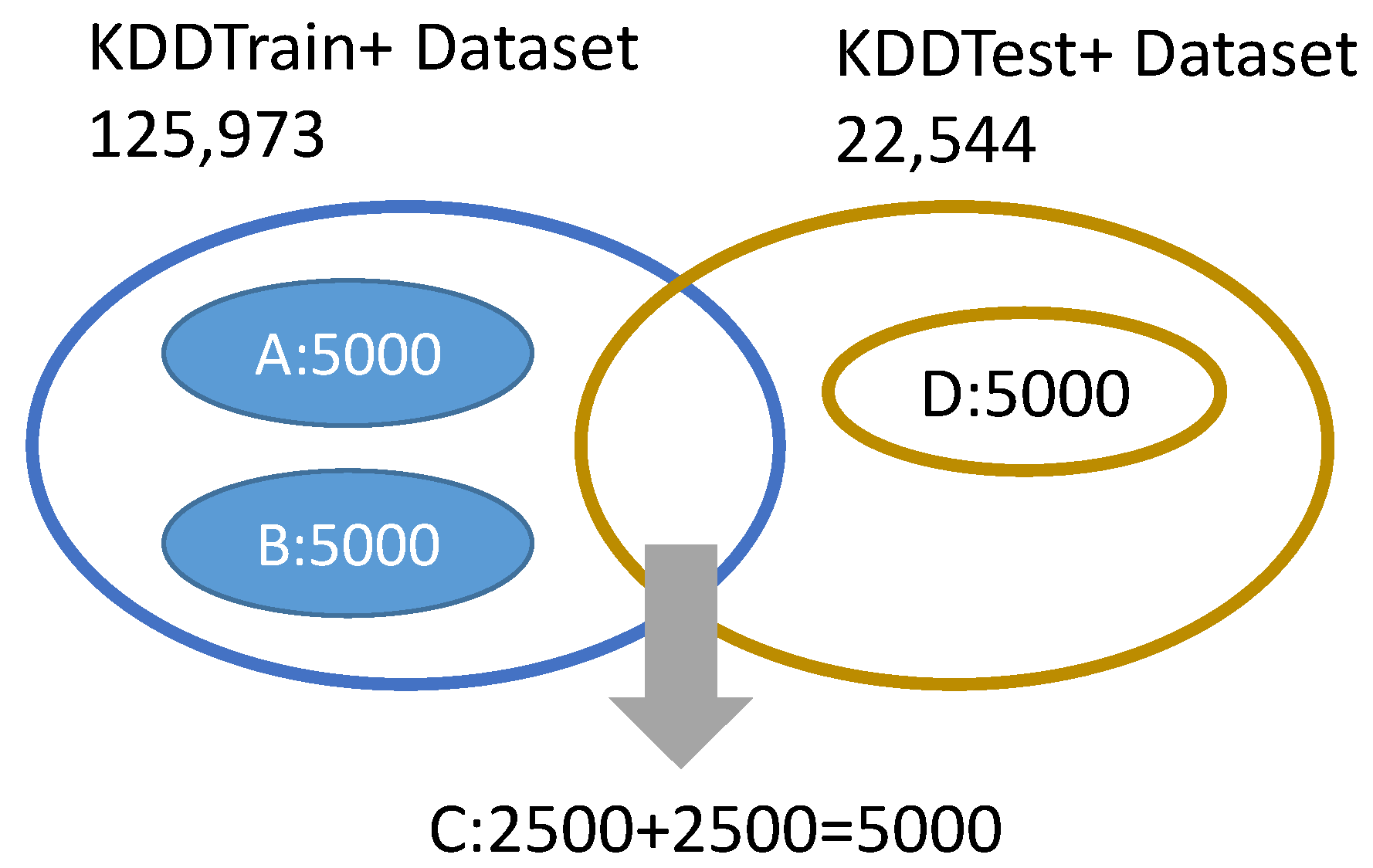
The NSL-KDD data set was used in this study and had the basic host feature content which included time and traffic. The training data set contained 22 different attacks. To simulate an actual situation, new attacks would appear. The test data set contained 17 attack types that had not appeared in the training dataset. The KDDTest+ and KDDTrain+ datasets, which have 22,544 and 125,973 network data records respectively, were used. The WEKA-ReSample tool was used for the sampling of four sub-datasets A, B, C, and D from the original (KDDTest+ and KDDTrain+) respectively, for use as experimental data set samples, as shown in Figure 1.

Each NSL-KDD network data record has 38 digital type attribute features, as well as three character type attribute features including protocol type, service, and flag. Furthermore, the protocol type has 3 features, service has 70 features, and flag has 11 features. It was therefore necessary to map and transform the character type features in the original record to digital feature attributes. The WEKA-Nominal to binary encoding method was used to encode the character features, turning each original data record into a 122-dimensional eigenvector. Since the data had significantly different resolutions and ranges, the range of value captured was not uniform. Therefore, standardization or mean removal and variance scaling was needed for each eigenvector. After the transformation, each dimension had a mean of 0, also called the Z-score normalization. Calculation involved subtraction of the mean (M) from feature (X) and division by the standard deviation (S) (calculation equation: Z = (X − M)/S), so the attribute data was scaled within a range of [0, 1]. After standardization of the training data set, the same procedure was used to standardize the test data set.

The Weka tool was used to load the sampled experimental data set (sub-data sets A, B, C, and D, each having 5000 records, and the random sampling reflected, as far as possible, the various information expected during the analysis) for data preprocessing, and PCA was used to reduce the number of features to 94. Four kinds of classification algorithms: SVM, naive Bayes, decision tree (J48), and MLP were used in the experimental tests. Data that had not been dimensionally reduced, and data which had been reduced, were both used. In the accuracy experiment for each group, data was compared in three different combinations. Data set A was used to train each group, data set B was used to test the first group, data set C was used for the second group, and data set D was used for the third group.

4.1. SVM Classifier Results

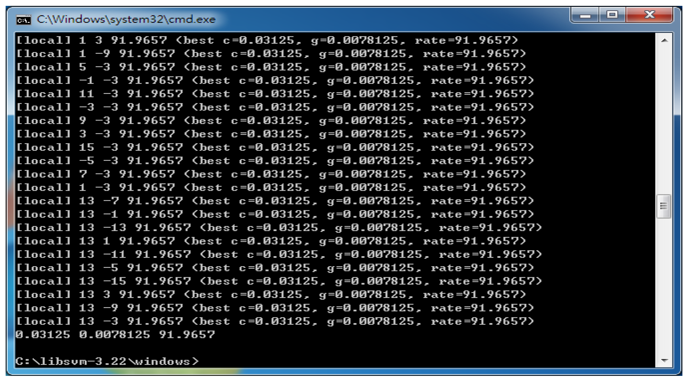
The SVM model has two very important parameters, C and gamma. Where C is the penalty factor, which is the tolerance for error. The higher the value of c, the less the tolerance and over-fitting is easy. The smaller the value of C, the easier it is to fit. If C is too big or too small, the generalization ability will suffer and become worse. Gamma is a parameter that comes with the function after selection of the RBF function as the kernel. It implicitly determines the distribution of data after mapping to a new feature space. The larger the gamma value, the smaller the support vector, the smaller the gamma, the larger the support vector. The number of support vectors affects the speed of training and prediction. In the process, we experimented with the parameters c and g settings, and used the parameter check program grid.py to find the best parameters c and g. After the program is executed, the last set of parameters is 0.03125, 0.0078125, and 91.9657 (Figure 2), where c = 0.03125, g = 0.0078125, the parameters c and g are brought into the SVM classifier respectively, the correct rate of training and test results are 92.2396% and 67.7032% respectively. After several parameter adjustment experiments, it was decided to use c = 1.0 and g = 0.0 as the best parameter values to verify with the other three classifiers in the paper.

Weka was used for pre-processing. Feature selection, dimension reduction to 94 features, and training and testing of the data set was done as before and according to the status of each data set. The kernel function (parameter setting: parameter gamma = 0.0, parameter C = 1.0) was applied including linear SVM, polynomial, RBF, and sigmoid for training and prediction, and the results are shown in

Table 2. Training and detection results for each SVM kernel function

Type of Classifier	Data	First Group (Correct Rate/Time)	Second Group (Correct Rate/Time)	Third Group (Correct Rate/Time)
SVM (Linear)	Original data	97.38%	81.74%	78.78%
		0.83 (s)	0.56 (s)	0.81 (s)
	Data after Dimension Reduction	96.68%	83.22%	80.72%
		0.81 (s)	0.78 (s)	0.78 (s)
SVM (Polynomial)	Original data	96.36%	77.12%	73.00%
		2.23 (s)	2.2 (s)	2.64 (s)
	Data after Dimension Reduction	93.58%	73.48%	69.82%
		6.07 (s)	5.13 (s)	5.16 (s)
SVM (RBF)	Original data	97.22%	82.34%	79.64%
		2.12 (s)	2.18 (s)	2.06 (s)
	Data after Dimension Reduction	96.40%	82.52%	79.72%
		1.72 (s)	1.76 (s)	1.65 (s)
SVM (Sigmoid)	Original data	94.46%	82.78%	78.32%
		1.04 (s)	0.97 (s)	1.47 (s)
	Data after Dimension Reduction	95.20%	82.88%	78.82%
		1.22 (s)	1.64 (s)	1.25 (s)

. It can be seen that the test of the first group had the best original data recognition. When used for recognition, the kernel of the RBF can reach 97.22%. The linear kernel recognition rate for the first group, after dimensionality reduction, can reach 96.68%. Although the SVM classifier showed no enhancement of recognition rate after dimension reduction, the calculation speed was substantially improved.

4.2. Naive Bayes Classifier Results

The results obtained with the Weka-naive Bayes classifier, using the default parameters are shown in

Table 3. Training and detection results for naive Bayes

Types of Classifier	Data	First Group (Correct Rate/Time)	Second Group (Correct Rate/Time)	Third Group (Correct Rate/Time)
Naive Bayes	Original data	90.00%	81.28%	80.90%
		0.67 (s)	0.61 (s)	0.61 (s)
	Data after dimension reduction	91.54%	79.94%	79.46%
		0.44 (s)	0.64 (s)	0.47 (s)

. The results indicate that, recognition of the data after dimension reduction was enhanced and the calculation speed also improved, achieving a 91.54% recognition rate and a calculation speed of 0.44 s.

4.3. J48 Classifier Results

The J48 algorithm has two important parameters: The first is C (the confidence factor) which is the level used to define the confidence interval. A lower C value will give a wider interval, meaning a more negative estimate, which will result in heavier pruning. The confidence factor value is the parameter basis for pruning after the decision tree has been established. The smaller the value, the more extensive the pruning. The second is the M parameter which is the minimum number of instances in the two most popular branches. The classifier displays the results in the text box next to the selection button, and shows (J48-C 0.05-M 2), (J48-C 0.25-M 2), (J48-C 0.4-M 2), (J48-C 0.05-M 50), (J 48-C 0.25-M 50), (J 48-C 0.4-M 50), (J 48-C 0.55-M 500), (J 48-C 0.25-M 500), (J 48-C 0.4-M 500) as the parameter settings. The results in

Table 4. J48 training and detection results

Type of Classifier	Data	First Group (Correct Rate/Time)	Second Group (Correct Rate/Time)	Third Group (Correct Rate/Time)
J48(C = 0.05, M = 2)	Original data	59.30%	51.08%	44.20%
		0.19 (s)	0.2 (s)	0.14 (s)
	Data after Dimension Reduction	48.32%	50.94%	51.08%
		0.13 (s)	0.14 (s)	0.11 (s)
J48(C = 0.25, M = 2)	Original data	59.30%	51.08%	44.20%
		0.16 (s)	0.2 (s)	0.17 (s)
	Data after Dimension Reduction	48.32%	53.02%	50.22%
		0.13 (s)	0.14 (s)	0.11 (s)
J48(C = 0.4, M = 2)	Original data	59.30%	51.08%	44.20%
		0.16 (s)	0.14 (s)	0.16 (s)
	Data after Dimension Reduction	48.32%	53.02%	50.22%
		0.11 (s)	0.14 (s)	0.11 (s)
J48(C = 0.05, M = 50)	Original data	52.30%	51.62%	44.70%
		0.16 (s)	0.16 (s)	0.17 (s)
	Data after Dimension Reduction	49.22%	52.64%	53.24%
		0.13 (s)	0.14(s)	0.11(s)
J48(C = 0.25, M = 50)	Original data	52.30%	51.62%	44.70%
		0.14 (s)	0.17 (s)	0.17 (s)
	Data after Dimension Reduction	49.22%	52.64%	53.24%
		0.11 (s)	0.16	0.14(s)
J48(C = 0.4, M = 50)	Original data	52.30%	51.62%	44.70%
		0.23 (s)	0.16 (s)	0.17 (s)
	Data after Dimension Reduction	49.22%	52.64%	53.24%
		0.11 (s)	0.16	0.11(s)
J48(C = 0.05, M = 500)	Original data	52.88%	67.12%	77.32%
		0.16 (s)	0.17 (s)	0.17 (s)
	Data after Dimension Reduction	86.02%	76.50%	76.06%
		0.13 (s)	0.16 (s)	0.11 (s)
J48(C = 0.25, M = 500)	Original data	52.88%	67.12%	77.32%
		0.14 (s)	0.17 (s)	0.17 (s)
	Data after Dimension Reduction	86.02%	76.50%	76.06%
		0.11 (s)	0.13 (s)	0.14 (s)
J48(C = 0.4, M = 500)	Original data	52.88%	67.12%	77.32%
		0.23 (s)	0.14 (s)	0.16 (s)
	Data after Dimension Reduction	86.02%	76.50%	76.06%
		0.14 (s)	0.16 (s)	0.11 (s)

show that the calculation speed tends to be fast, but the recognition rate is generally poor, and the data after dimension reduction (J48-C 0.05 to 0.4-M 500) had the best recognition rate, reaching 86.02%.

4.4. MLP Classification Test Results

The Weka-MLP tool was used to do the MLP classification test. The parameters were the number of hidden units (2 or 4), the ridge factor for quadratic penalty on weights (default 0.01), the tolerance parameter for delta values (default 1.0 × 10⁻⁶), conjugate gradient descent was used (recommended for many attributes), the size of the thread pool (default 1), the number of threads to use (default 1), and random number seed (default 1). Tests were done for four combinations according to the parameters, the combinations were AA (approximate sigmoid and approximate absolute error), AS (approximate sigmoid and squared error), SA (soft plus and approximate absolute error), and SS (soft plus and squared error). The results in

Table 5. MLP training and detection results

Type of Classifier	Data	First Group (Correct Rate/Time)	Second Group (Correct Rate/Time)	Third Group (Correct Rate/Time)
MLP (N = 2)	Original data	97.74%	78.84%	75.84%
		0.19 (s)	0.16 (s)	0.17 (s)
	Data after dimension reduction	97.18%	83.12%	79.10%
		0.31 (s)	0.36 (s)	0.17 (s)
MLP (N = 4)	Original data	97.76%	81.54%	78.98%
		0.23 (s)	0.17 (s)	0.16 (s)
	Data after dimension reduction	97.24%	81.44%	78.40%
		0.27 (s)	0.22 (s)	0.38 (s)
AS Training (Activation Functions: Approximate Sigmoid Loss Functions: Squared Error)
Type of Classifier	Data	First group (Correct Rate/Time)	Second Group (Correct Rate/Time)	Third Group (Correct Rate/Time)
MLP (N = 2)	Original data	97.76%	78.86%	76.06%
		0.16 (s)	0.16 (s)	0.17 (s)
	Data after dimension reduction	97.24%	80.78%	77.56%
		0.12 (s)	0.19 (s)	0.17 (s)
MLP (N = 4)	Original data	97.62%	85%	81.76%
		0.17 (s)	0.17 (s)	0.17 (s)
	Data after dimension reduction	97.82%	84.56%	79.32%
		0.17 (s)	0.17 (s)	0.19 (s)
SA Training (Activation Functions: Soft Plus Loss Functions: Approximate Absolute Error—E 0.01)
Type of Classifier	Data	First Set of Tests (Correct Rate/Time)	Second Set of Tests (Correct Rate/Time)	Third Set of Tests (Correct Rate/Time)
MLP (N = 2)	Original data	97.64%	79.92%	75.74%
		0.17 (s)	0.16 (s)	0.17 (s)
	Data after dimension reduction	94.38%	81.40%	77.26%
		0.27 (s)	0.19 (s)	0.16 (s)
MLP (N = 4)	Original data	95%	77.96%	72.18%
		0.19 (s)	0.16 (s)	0.27 (s)
	Data after dimension reduction	94.56%	81.12%	75.98%
		0.14 (s)	0.17 (s)	0.14 (s)
SS training (Activation Functions: Soft Plus Loss Functions: Squared Error)
MLP (N = 2)	Original data	97.52%	78.88%	76.68%
		0.14 (s)	0.17 (s)	0.17 (s)
	Data after dimension reduction	97.76%	79.90%	79.28%
		0.13 (s)	0.23 (s)	0.14 (s)
MLP (N = 4)	Original data	97.92%	78.92%	75.80%
		0.16 (s)	0.17 (s)	0.16 (s)
	Data after dimension reduction	97.52%	80.84%	77.34%
		0.14 (s)	0.19 (s)	0.17 (s)

show that the highest recognition rate was 97.82%, and when number of hidden units was 4, and approximate sigmoid and squared error had also been selected, the calculation speed was 0.17 s.

4.5. Correlation of Recognition Rate between the Classification Methods and Reduction of Dimension

PCA was used for feature selection and to reduce the dimension of available attributes in the data set from 122 to 94. Classification was done by SKA, naive Bayes, J48, and the MLP algorithms through WEKA. Correlation of each kind of classification algorithm and dimension reduction was carried out, and

Table 6. Detection accuracy of the classifiers of the different algorithms

Algorithm		Test Classification
		First Set of Tests (Correct Rate/Time)	Second Set of Tests (Correct Rate/Time)	Third Set of Tests (Correct Rate/Time)
SVM-RBF	Original data (122 Features)	97.22%	82.34%	79.64%
		2.12 (s)	2.18 (s)
	Data after dimension reduction (94 Features)	96.4%	82.52%	79.72%
		1.72 (s)	1.76 (s)	1.65 (s)
Naive Bayes	Original data (122 Features)	90%	81.28%	80.9%
		0.67 (s)	0.67 (s)	0.61 (s)
	Data after dimension reduction (94 Features)	91.54	79.94	79.46
		0.44 (s)	0.64 (s)	0.47 (s)
J48 (C = 0.25, M = 2)	Original data (122 Features)	59.3%	51.08%	44.2%
		0.16 (s)	0.2 (s)	0.17 (s)
	Data after dimension reduction (94 Features)	48.32%	53.02%	50.22%
		0.13 (s)	0.14 (s)	0.11 (s)
MLP-AS (N = 4)	Original data (122 Features)	97.62%	85%	81.76%
		0.17 (s)	0.17 (s)	0.17 (s)
	Data after dimension reduction (94 Features)	97.82%	84.56%	79.32%
		0.17 (s)	0.17 (s)	0.19 (s)

shows the correct rate of classification detection for each data set and the parameter settings.

From the results, it can be clearly seen that the greater the amount of PCA dimension reduction, the faster the calculation speed. The reduction had no absolute correlation with the correct rate. When the classifier and parameter MLP-AS was N = 4, the same dimensionality reduction did not significantly improve the recognition rate. The MLP calculation speed was not improved either. However, its recognition rate was the highest among the classifiers, reaching 97.82%. The results of SVM-RBF are similar to those of MLP.

5. Conclusions

The increase in the number and severity of network attacks in recent years has made APT detection a vital matter and it has become the key to network security protection. A large amount of security audit data and the complex and dynamic features of intrusion behavior, as well as optimization of the performance of APT detection has become an important open issue. This has attracted much attention from the information security and academic research communities. According to the experiments in this study, the classifiers SVM-RBF and MLP-AS (N = 4) have the best recognition rate for NSL-KDD. Using PCA to reduce the dimension did not help with the recognition rate, but it could improve the calculation speed. It is recommended that SVM-RBF or MLP-AS (N = 4) classifiers be used for the detection of an APT attack. There is an advantage to using SVM and PCA together to accelerate the calculation process. The experimental results of this study provide reference models for follow-up research in the selection of classifiers and parameters, information about the effects of the reduction of dimensionality and calculation speed, as well as a better understanding of the contents of the data set.

Many of the network intrusion detection system modules used today are modeled using the support vector machine algorithms. However, they are very demanding in terms of system computing hardware performance. To alleviate this problem, dimension reduction is applied to a given data set that uses important feature extraction to improve processing speed. Data from the experimental results show that data dimensionality reduction had no significant impact on the results but detection speed was enhanced. Improvements in the characteristic information of the data set content used to analyze the APT attack, as well as in the dimensionality reduction method, will further improve the accuracy of effective analysis.