An FCM–GABPN Ensemble Approach for Material Feeding Prediction of Printed Circuit Board Template

Featured Application

The application of the work is to optimize the material feeding of a printed circuit board (PCB) template and therefore reduce the comprehensive cost caused by surplus and supplemental feeding.

Abstract

Accurate prediction of material feeding before production for a printed circuit board (PCB) template can reduce the comprehensive cost caused by surplus and supplemental feeding. In this study, a novel hybrid approach combining fuzzy c-means (FCM), feature selection algorithm, and genetic algorithm (GA) with back-propagation networks (BPN) was developed for the prediction of material feeding of a PCB template. In the proposed FCM–GABPN, input templates were firstly clustered by FCM, and seven feature selection mechanisms were utilized to select critical attributes related to scrap rate for each category of templates before they are fed into the GABPN. Then, templates belonging to different categories were trained with different GABPNs, in which the separately selected attributes were taken as their inputs and the initial parameter for BPNs were optimized by GA. After training, an ensemble predictor formed with all GABPNs can be taken to predict the scrap rate. Finally, another BPN was adopted to conduct nonlinear aggregation of the outputs from the component BPNs and determine the predicted feeding panel of the PCB template with a transformation. To validate the effectiveness and superiority of the proposed approach, the experiment and comparison with other approaches were conducted based on the actual records collected from a PCB template production company. The results indicated that the prediction accuracy of the proposed approach was better than those of the other methods. Besides, the proposed FCM–GABPN exhibited superiority to reduce the surplus and/or supplemental feeding in most of the case in simulation, as compared to other methods. Both contributed to the superiority of the proposed approach.

1. Introduction

Printed circuit board (PCB) is found in practically all electrical and electronic equipment, being the base of the electronics industry [1]. Due to the rapid development of computer, communication, consumer electronics, 5G, and automotive electronics, as well as the update of their products, the demand of PCB orders with specialized design features and manufacturing requirements, often referred to as a PCB template in the factory, has increased rapidly. The mode of production for a PCB factory with lots of template orders has changed from mass production to customer-oriented small-batch production, and therefore causes companies to face serious challenges. Accurate prediction of material feeding for each order is one of the critical problems.

After the feeding area and production panel (production unit) of each template order is accurately predicted, several goals (including the reduction of comprehensive cost caused overproduction or supplemental feeding, alleviation of environment pollution, improvement of on-time delivery, etc.) can be simultaneously achieved. However, it is difficult to determine the material feeding area of each PCB template order in advance of the production by manual feeding. Many factories undergo the violent fluctuation in both surplus and supplemental feeding by empirical manual feeding. Individualized surplus templates can be placed only in inventory or directly disposed, while supplemental feeding brings extra production costs and increases the probability of delivery tardiness compensation [2]. Furthermore, surplus products bring extra chemical and heavy metal pollution for production and disposal. This motivates us to explore the pattern of historical records that facilitate more reasonable and accurate prediction of material feeding for new template orders.

There are many applications of data mining (DM) or big data for quality improvement and optimization of PCB production [3]. Lee et al. [4] developed a data mining (DM)-based approach to predict the yield of a PCB, using the event sequence. Tsai [5] proposed a hybrid DM approach for soldering quality classification by using self-organizing map (SOM) and K-means, based on the statistical process control databases. DB-based PCB manufacturing process optimization has also attracted many researches, such as the parameter optimization of hot solder dip [6], stencil printing process [7,8], reflow soldering [9,10], fluid dispensing for microchip encapsulation [11], and wave soldering [12,13] for a component surface mount on a PCB. These models always combined artificial neural network (ANN), support vector machine (SVM), and multiple linear regression (MLR) for quality prediction with GA for parameters optimization simultaneously [7,10,11]. Meanwhile, many DM approaches like adaptive genetic algorithm (GA)-artificial neural network (ANN) [14], decision tree (DT) [15] have been employed for the defect diagnosis of PCB. The DM and/or big data were also widely adopted for smart production in different industries, not only for PCB manufacturing, and many reviews of these applications were reported in recent two years [3,16,17]. However, few of the aforementioned studies are on the prediction and optimization of material feeding in PCB template orders. In addition, the reviewed studies seldom considered the situation of diverse examples with different critical influence factors that require different prediction models to improve the prediction accuracy.

Considering the abovementioned requirement of a PCB template, Lv et al. [2] developed a hybrid model, multiple structural change (MSC)–ANN, to predict the feeding panel for each template, in which the template samples were pre-classified based on the required panel by the multiple structural change model. Then, the critical attributes for each category were selected based on neighborhood component approach; finally, the ANN prediction models were established for each category. The experimental results indicated that the attempt of the pre-classifying of inputs and establishing a prediction model for each category can indeed improve the prediction accuracy of material feeding for PCB template production. However, the MSC–ANN considered only one attribute to classify the sample, and the attributes were selected for each category by only one feature selection approach. Meanwhile, a template might be partitioned into multiple categories with different degrees, while the pre-partition based on MSC is a hard clarification. Therefore, it seems to be insufficient to predict the production-feeding panel of each template by using a prediction approach suited to a single category. Besides, MSC–ANN cannot handle a template order belonging to the border of two adjacent categories, because neither of the prediction models for the two categories is suitable for the template. Furthermore, the initialization parameter optimization of ANN benefits accuracy improvement [11,18,19] but was not considered.

For tackling the aforementioned difficult problems, a fuzzy c-means (FCM) classifier was adopted to handle the fuzzy classification and back-propagation network (BPN) ensemble with an aggregator BPN was employed to tackle the prediction by considering the membership degree of each template. The linear correlation (LC) [20], maximum information coefficient (MIC) [21], recursive feature elimination (RFE) [22], LR [23], lasso regression [24], ridge regression [25], and random forest regression (RFR) [26] seven feature selection approaches were taken to select the critical attributes of each category divided by FCM. The GA was used to optimize the initialization parameters of BPN for each category. The reason for employing an FCM is that it accounts for the flexible classification (a template might be clustered into multiple categories with different membership degrees) and was widely used in many fields [27,28,29]. The reason for applying GA is that GA is easy to encode the problem and achieve good optimization results. It was also widely employed to optimize the structure (the number of layers and nodes in each hidden layer) and/or initial weight and bias [18,19,30] for the purpose of improving the prediction effectiveness of BPN. An aggregator BPN was adopted to conduct nonlinear aggregation because, theoretically, a BPN can approximate any nonlinear relationship [31].

In the proposed FCM–GABPN approach, input samples were first clustered with FCM, and seven feature selection methods were utilized to select critical attributes related to scrap rate for each category (a cluster is taken as a category) of PCB templates before they were fed into the BPN. Then, samples belonging to different categories were trained with different BPNs, in which the separately selected attributes were taken as their inputs and the initial parameters were optimized with GA. After training, an ensemble predictor formed with all GABPNs was taken to predict the scrap rate. Finally, another BPN was adopted to conduct nonlinear aggregation of the outputs from the component BPNs and determine the predicted feeding panel of the PCB template with a transformation. The proposed FCM–GABPN approach is illustrated in Figure 1.

The remainder of the paper is organized as follows. In Section 2, variables specification and sample collection are described. The FCM, feature selection methods, GABPN, and the nonlinear aggregation BPN are introduced in Section 3, followed by experimental results and discussion in Section 4. Lastly, conclusions are given in Section 5.

2. Variables and Sample

The data used in this study were collected from Guangzhou FastPrint Technology Co., Ltd. A total of 56 variables inherited from an enterprise resource planning system combined with the derived variables were selected and specified in

Table 1. Variables specification.

No.	Variable Name	Symbol	Description	Value Range
Overall characteristics
1	PCB thickness (mil)	Pt	Thickness of the ordered PCB	0.3–8
2	Layer number	Ln	Number of copper layer.	4–20
3	Rogers material	Ro	Whether substrate material is Rogers.	0/1
4	Plating frequency	Plfr	Number of plating operation.	0–4
5	Number of operations	Noo	Number of operations to produce the order.	16–71
6	Number of Prepreg	NPP	Number of Prepreg for lamination	1–50
7	Scrap units in a set	Sus	Allowed maximum scrap units in a set.	0–8
8	Photoelectric board	Photb	Whether the order is the specified board.	0/1
9	High frequency board	Highfb
10	Test board	Semictb
11	Negative film plating	Nflp	Whether the order takes negative film plating.
12	Tinning copper	Tinc	Whether the order has tinning copper.
13	IPCIII standard	IPCIII	Whether the order takes IPCIII or Huawei standard.
14	Huawei standard	Huawei
Feature of internal/outer layer line
15	Minimum line width in internal layer (mil)	Mwil	Minimum line width or space in core boards	3–100
16	Minimum line space in internal layer(mil)	Mlsil		1–137.66
17	Minimum line width in outer layer(mil)	Mwol	Minimum line width or space in outer layer	1–157.5
18	Minimum line space in outer layer (mil)	Mlsol		1.2–290
19	Average residual rate	Arcr	Average residual rate of copper layer	0.15%–94.75%
Feature and operation information of hole
20	Solder resist plug hole	Srph	Whether the order has the specified hole related operation.	0/1
21	Plug hole with resin	Phwr
22	Second drilling	Secd
23	Back drilling	Bcdr
Operation information of character/solder mask
24	Character print	Chaprt	Whether the order has the specified character/solder mask related operation.	0/1
25	White oil solder mask	White
26	Blue oil solder mask	Blue
27	Black oil solder mask	Black
Surface finishing operation options
28	Hot-air solder leveling	Hasl	Whether the order takes the specified surface finishing operation.	0/1
29	Lead-free hot air solder leveling	Lfhasl
30	Entek	Osp
31	Cu/Ni/Au pattern plating	Cnapp
32	Gold finger plating	Gfig
33	Gold plating	Godp
34	Soft Ni/Au plating	Snap
35	Immersion Ag/Sn/Au	Iasa
Statistic items
36	Delivery unit in a panel	Duap	Number of delivery unit in a panel	1–262
37	Supplemental feeding frequency	Supff	Material feeding frequency minus 1	0–14
38	Required quantity	Reqq	Demand quantity of delivery unit minus delivery unit in inventory for the same order No.	1–3000
39	Required panel	Reqp	Reqq/Duap rounded up to the nearest integer	1–225
40	Feeding quantity	Fedq	Feeding number of delivery unit	2–6296
41	Least feeding panel	Lfp	Reqq/(1-scrap rate) rounded up to the nearest integer	1–245
42	Feeding panel	Fedp	Number of feeding panel	1–308
43	Scrap quantity	Scraq	Scrap number of delivery unit	0–712
44	Qualified quantity	Qualq	Qualified number of delivery unit	1–6226
45	Surplus quantity	Surpq	Qualq–Fedq	0–3226
46	Delivery unit area(m2)	Dunita	Area of a delivery unit	0.001–0.393
47	Required area(m2)	Reqa	Reqq × Dunita	0.001–25.74
48	Feeding area(m2)	Feda	Fedq × Dunita	0.011–42.63
49	Scrap area(m2)	Scraa	Scraq × Dunita	0–15.39
50	Qualified area(m2)	Quala	Qualq × Dunita	0.009–37.49
51	Surplus area(m2)	Surpa	Surpq × Dunita	0–25.45
52	Supplemental feeding rate	Supfr	Supff in a certain period/number of orders × 100%	18.83%
53	Scrap rate	Scrar	Scraa/Feda × 100%	0%–68.48%
54	Qualified rate	Qualr	Quala/Feda × 100%	31.52%–100%
55	Surplus rate	Surpr	Surpa/Reqa × 100%	0%–554.22%
56	Historical qualified rate	Hquar	The Qualr for the same order No. in the past 2 years	8.824%–100%

Note: New orders having no Hquar are replaced by the Qualr for orders having the same layer number and surface-finishing operation during the past 2 years.

, in which variables 1 to 35 are the product/process attributes, while 36 to 56 are the statistic variables. The delivery unit in a panel, required quantity/panel/area, and delivery unit area, with No. 36, 38, 39, 47, and 46, respectively, can not only be taken as statistic items, but also attribute candidates for prediction model establishment. Set and unit are two types of delivery unit, whereas panel as a production unit will be partitioned into either set or unit according to the customer’s requirement before delivery. If the number of final qualified set/unit (feeding set/unit minus the scrap set/unit) is larger than the demand number, it brings surplus sets/units; conversely, it causes supplemental feeding.

On this basis, 30,117 samples of the orders were collected, multivariate boxplots [2] were conducted to detect the outliers, and, finally, 29,157 samples were left for this study. Performances of the proposed FCM–GABPN are compared to the other five approaches based on the same samples. Value range in the last column of Table 1 is the statistic result of the 29,157 samples, and variables 40 to 56 are the statistic results of the manual feeding adopted by FastPrint.

3. Methodology

The procedure of the proposed approach (FCM–GABPN) is shown in Figure 2, and various aspects of FCM–GABPN are discussed in the following subsections.

3.1. Data Preparation and Template Classification with FCM

Data preparation is to collect the historical data of PCB templates for this study based on the variables given in Table 1. Then, 0–1 normalization was conducted for each variable for the purpose of reducing the influence of value-range difference. On this basis, the input attributes for FCM were selected based on the experience of experts from PCB workshops. The 17 attributes marked with boldface type in Table 1 were selected, in which the attributes of Ln and Noo represent the overall characteristics of the template; the Mwil, Mlsil, Mwol, and Mlsol are the design requirements of the hole and line; and the Reqq, Reqp, and Reqa are the production scale of each template order. Others are surface-finishing operation options.

Samples of templates were pre-classified into K categories with the selected 17 attributes by FCM before they were fed into the BPN. One recent example of FCM application is Tang et al. [27], in which FCM combining with adaptive neural network was applied to predict the lane changes by considering different simulation scenarios, and the results showed that the prediction performance and stability was considerably improved when compared with ANN, SVM, and MLR. Besides, Rezaee et al. [28] incorporated a dynamic FCM in ANN for the online prediction of companies in the stock exchange. According to experimental results, Rezaee et al.’s algorithm was efficient at clustering samples. In addition, Fathabadi [29] applied dynamic FCM clustering based ANN approach to reconfigure power-distribution networks. Experimental results indicated that Fathabadi’s approach has some benefits, such as a short process time, a very simple structure, and higher accuracy compared to the others.

FCM performs clustering by minimizing ${\displaystyle \sum _{c=1}^C{\displaystyle \sum _{i=1}^n{\mu }_{i(c)}^m{e}_{i(c)}^2}}$, where C is the required number of clusters; n is the number of samples; ${\mu }_{i(c)}^{}$ represents the membership of sample $i$ belonging to cluster $c$; $e_{i(c)}^{}$ measures the distance from samples $i$ to the centroid of $c$; $m\in (1,\infty )$ is the hyper-parameter that controls how fuzzy the cluster will be. The procedure of applying FCM to cluster samples is as follows [31]:

(1)

The cluster membership value, $u_{ij}^{}$ (the coefficient giving the degree of $x_i$ being in the j^th cluster), are initialized randomly and establish an initial clustering result.

(2)

(Iterations) obtain the centers of each cluster as ${\overline{x}}_{(c)}=\left\{{\overline{x}}_{(c)j}\right\}$, ${\overline{x}}_{(c)j}={\displaystyle \sum _{i=1}^n{u}_{i(c)}^m{x}_{ij}}/{\displaystyle \sum _{i=1}^n{u}_{i(c)}^m}$, $1\le j\le 17$, $u_{i(c)}=1/{\displaystyle \sum _{i=1}^C{(e_{i(c)}^{}/e_{i(c)}^2)}^{2/(m-1)}}$, $e_{i(c)}^{}=\sqrt{{\displaystyle \sum _{allj}{(x_{ij}-{\overline{x}}_{(c)j})}^2}}$, where $x_{ij}$ is the j^th variable of the selected 17 attributes of sample i, and${\overline{x}}_{(c)}$ is the centroid of cluster c.

(3)

Re-measure the distance of each PCB template to the centroid of every cluster, and then recalculate the corresponding membership value.

(4)

Stop if the number of iterations is larger than a set value. Otherwise, return to Step (2).

After clustering, samples of different categories (clusters) are then trained with different BPNs. First, a membership threshold value ${\mu }_L$ for selecting samples in network learning has to be determined. Only samples with ${\mu }_{i(c)}^{}\ge {\mu }_L$ will be taken in training the BPN to obtain the weights and bias geared to the $c^{th}$ category. As a result, a sample might be selected by multiple categories.

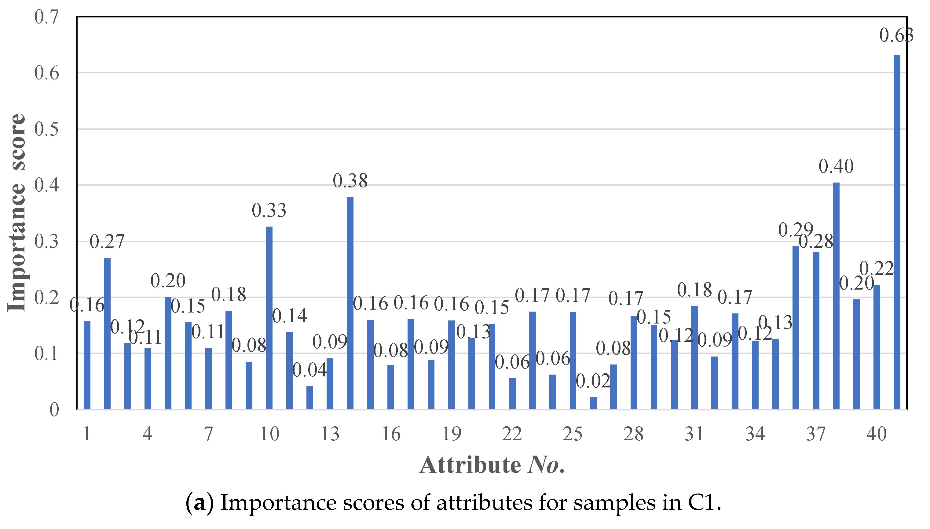
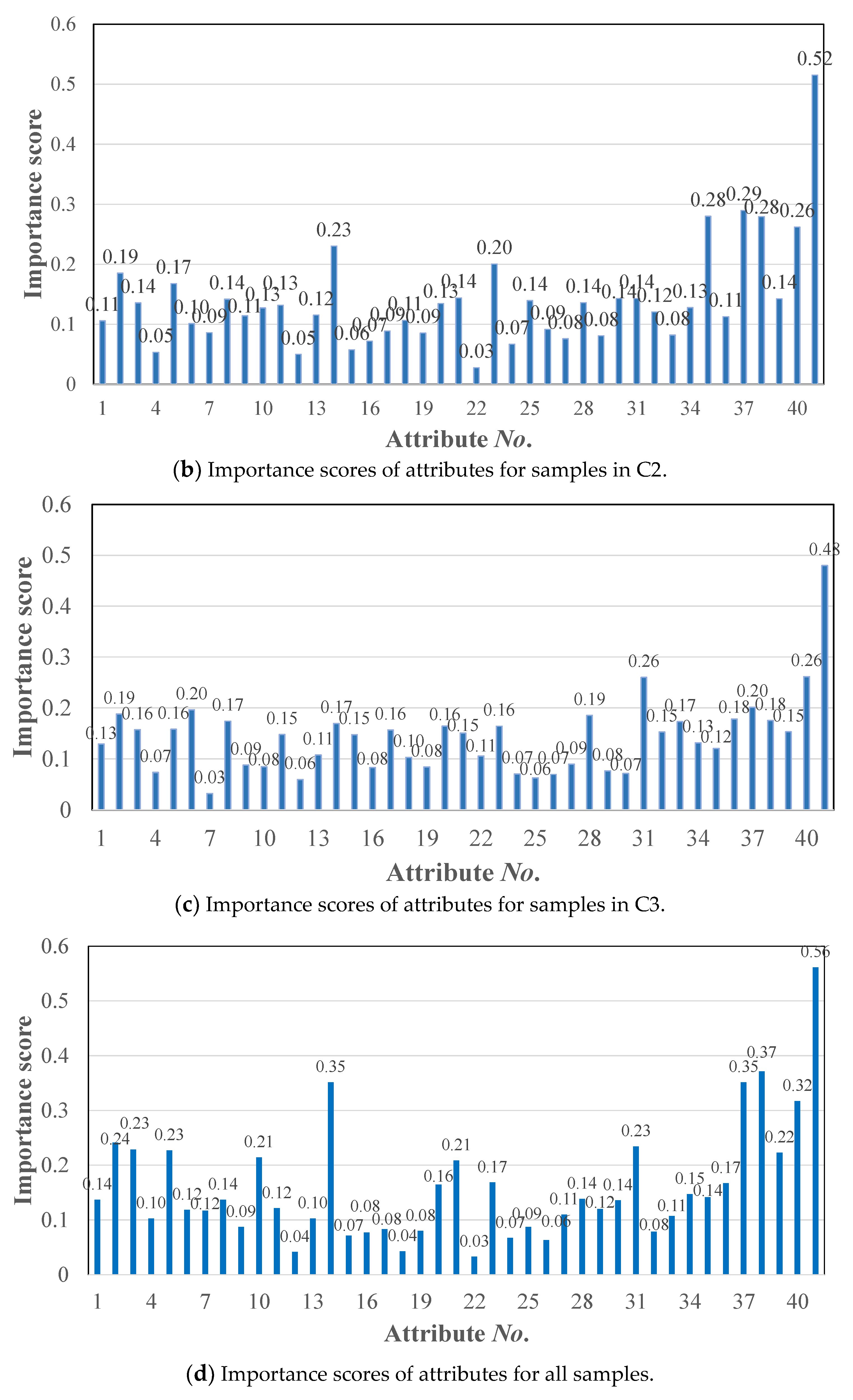
3.2. Attributes Selection for Each BPN Prediction Model

It is necessary to remove irrelevant and redundant attributes to reduce the complexity of analysis and the generated models, and also improve the efficiency of the whole modelling processes [2,32]. In this study, LC [20], MIC [21], RFE [22], LR [23], lasso regression [24], ridge regression [23], and RFR [24] seven feature selection approaches were employed to select critical attributes related to the scrap rate for each category of samples. The scarp rate can be taken as the dependent variable, and the independent variables are the attributes with No. 1–36, 38, 39, 46, and 47, given in Table 1. The score of independent variables obtained by each feature selection method were calculated and whose average score is greater than a certain threshold (e.g., 0.15) were taken as the input attribute of the prediction model.

The LC uses the linear correlation coefficient $lcc(x,y)=\mathrm{cov}(x,y)/\sqrt{\mathrm{var}(x)\mathrm{var}(y)}$ to measure the relationship between the (independent) variable x and variable y, where var is the variance of a variable and cov(x, y) denotes the covariance between x and y (namely scrap rate here) [20]. MIC is based on the idea that if a relationship exists between two variables, then a grid can be drawn on the scatterplot of the two variables that partition the data to encapsulate the relationship. To calculate the MIC of a set of two-variable data, all grids up to a maximal grid resolution are explored by computing for every pair of integers (x, y) the largest possible mutual information achievable by any x-by-y grid applied to the data. Then these mutual information (MI) values are normalized to ensure a fair comparison between grids of different dimensions and to obtain modified values between 0 and 1. Finally, the highest normalized MI achieved by any x-by-y grid as the value of MIC [21]. The main idea of RFE is to train an estimator based on the initial set of variables and weights are assigned to each one of them at first. Then, variables whose absolute weights are the smallest are pruned from the current set of variables. That procedure is recursively repeated on the pruned set until the desired number of variables to select is eventually reached [22].

The LR is to establish the regression equation of the dependent variable based on the independent variables, in which the importance of independent variables will be determined according to F-test. The smaller the value of F-test, the more important the variable is to the regression equation [21]. The lasso regression is a regularized LR by putting a L1 norm penalty on the regression coefficients. Lasso regression will drive more coefficients of weak correlated independent variables to zero, and then facilitate the selection of variables with strong correlation [24]. The ridge regression is similar to lasso regression by putting a L2 norm penalty on the regression to penalize the weak correlated variables for the regression model establishment [25]. RFR is an ensemble of unpruned classification or regression trees, in which each branch of the trees will calculate the importance of each unused attribute in previous steps and then facilitate important-attribute selection simultaneously [26]. The above seven approaches were realized by the encapsulated functions in the machine learning library “sklearn” in this study.

3.3. GABPN-Based Scrap Rate Prediction for Each Category

The configuration of the BPN is established as follows:

(1)

Input: the 0–1 normalized data of the selected attributes for each category.

(2)

Architecture: Single hidden layer (number of nodes in the input layer + number of nodes in the output layer)/2 is one of the commonly used ways to determine the suitable number of neurons in the hidden layer. Therefore, the number of nodes in hidden layer is depended on the number of selected attributes in this study. In order to achieve better prediction accuracy (a large number of the hidden-layer nodes are theoretically conducive to improve the predicting accuracy) and to keep the consistency, the number of neurons in the hidden layer of each BPN was set to 12 for each category in the proposed approach, considering the number of selected attributes (up to 23 selected attributes for the samples that will be discussed in Section 4).

(3)

Output: normalized scrap rate forecast of the template.

(4)

Learning rule: Delta rule (the adjustment of weight and bias is proportional to the negative gradient of the error during the backward-propagation procedure).

(5)

Propagation function: sigmoid activation function, $f(x_j)=1/(1+e^{-x_j})$.

(6)

Learning rate: 0.05.

(7)

Number of iterations: 25,000.

The performance of a BPN is sensitive to the initial condition. Therefore, the optimization of the initial weights and biases of BPN with GA was conducted. The design and configuration of GA is as follows:

(1)

Encoding and decoding: The individual chromosome in the population was encoded as $[W_1,{\Phi }_1,W_2,{\Phi }_2]$ in which $W_1=[w_{1,1},w_{1,2},\mathrm{..},w_{1,12},w_{2,1},w_{2,2},\mathrm{..},w_{2,12},w_{i,1},w_{i,2},\mathrm{..},\mathrm{..},w_{i,12}]$ (selected i attributes as input and the number of neurons in the hidden layer is 12) represents the weights between nodes in input layer and hidden layer; $W_1=[w_{1,1},w_{2,1},\mathrm{...},w_{12,1}]$ represents the weights between the nodes in hidden layer and output layer; ${\Phi }_1=[{\theta }_1,{\theta }_2,\mathrm{...},{\theta }_{12}]$ is the bias vector of nodes in the hidden layer; and ${\Phi }_2$ is the bias of output node. The decoding is to assign corresponding weights and bias to each node based on the BPN structure, and then conduct the forward propagation to compute the output of each BPN.

(2)

Population initialization: Each individual chromosome in the population was initialized randomly with its elements between −3 and 3, based on the encoding principle.

(3)

Fitness evaluation: The sum of absolute error between reversely normalized scrap rate forecast ${\widehat{o}}_k$ and actual scrap rate $o_k$ was taken as the fitness $F={\displaystyle \sum \left|{\widehat{o}}_k-o_k\right|}$ for each individual. The smaller the fitness is, the more accurate prediction result it can obtain. Thereafter, the minimization objective function, which the problem seeks to optimize, is the same as the fitness function.

(4)

Reproduction, crossover and mutation operation:

Reproduction: The roulette wheel selection was taken to select individuals for reproduction in which the fittest individuals have a greater chance of survival than weaker ones. The probability of each individual being selected is $p_i=(1/F_i)/{\displaystyle {\sum }_{j=1}^N(1/F_j})$, where $F_i$ is the fitness of the ith individual and N is the number of individuals.

Crossover: Two empty offspring chromosomes, O1 and O2, were initialized first, and two chromosomes, P1 and P2, were randomly selected from the reproduced population. The crossover location was randomly selected, and then the offspring O1 consisted of the genes of P1 before the crossover location and genes of P2 after the crossover location; while offspring O2 consisted of the genes of P2 before the crossover location and genes of P1 after the crossover location.

Mutation: One-point mutation was utilized as the mutation operator. The chromosome in the population was randomly selected, and one gene was chosen randomly from the selected chromosome. Then, a random r with the value in (0, 1) was generated to mutate the value. If $r>0.5$, then $a_j=a_j+(a_j-a_{\max })\times r$, otherwise $a_j=a_j+(a_{\min }-a_j)\times r$, where $a_j$ is value of the j^th position in the chromosome selected for mutation, and $a_{\max }$ and $a_{\min }$ are the maximum and minimum of the j^th position of all chromosomes in current generation, respectively.

(5)

Number of iterations: 100.

After the templates were clustered, a portion of the templates in each category were taken as “training samples” into the GABPN to determine the weights and bias values for the category. Three phases were involved at the training stage. First, the initial weight and bias were optimized according the GA. Second, the forward propagation is conducted, in which the inputs (selected attributes with bias) were multiplied with weights (weights of bias are 1), summated, and transferred to the hidden layer. The results of nodes in the hidden layer were further processed by sigmoid function and also transferred to the output layer with the same procedure. Finally, the output of GABPN was compared with the accurate scrap rate, and the accuracy of the GABPN, represented with mean squared error (MSE), was evaluated.

Subsequently, the backward pass which propagates derivatives (error between prediction and the actual value) from the output layer to hidden layers was conducted. The backward pass for a 3-layer BPN starts by computing the partial derivative for the output node (only one node here), and the error terms ${\delta }_j$ of nodes j in the hidden layers can be calculated according to ${\delta }_j=e{W}_j{f}^{\prime }(x_j)$, in which $e$ is error of the output node, $W_j$ is the weight connecting node j to the output node, and $f^{\prime }(x_j)$ is the derivative of the sigmoid activation function with the input $x_j$. On this basis, adjustments were made to the connection weights and bias to reduce the MSE. Network-learning stops when the iteration is greater than a given number in this study.

The trained GABPN was tested by the remaining portion of the templates in each category with the same performance indicator, MSE. Finally, the GABPN was used to predict the scrap rate of new templates that “completely” belonged to the clustered category. However, complete assignment of template to only a category is usually impossible. When a new template order is coming, the selected attributes associated with the new template are recorded, and the membership belonging to each category is calculated. Then, an ensemble predictor formed with all GABPNs can be taken to predict the scrap rate for the new template.

3.4. Nonlinear Aggregation with Another BPN and Transformation

For aggregating the predicted results from the component GABPNs into a single value representing the predicted scrap rate of the template, another BPN was employed in this study to conduct nonlinear aggregation, and the configuration is set as follows:

(1)

Input: 2K parameters consisted of the predicted results of each component GABPNs for the template and the membership values of the template belonging to each category.

(2)

Architecture: Single hidden layer and the number of nodes in the hidden layer were set to the same as that in the input layer, 2K.

(3)

Output: normalized scrap rate forecast of the template.

(4)

Learning rule: Delta rule.

(5)

Propagation function: sigmoid activation function.

(6)

Learning rate: 0.05.

(7)

Number of iterations: 10000.

The BPN also underwent training and testing. Then, the network output (i.e., the aggregation result) determined the normalized scrap-rate prediction of the template. Finally, the transformation of scrap rate to surplus rate and supplemental feeding rate were carried out. The reverse normalization was conducted for the output of the aggregation BPN and taking it as the predicted scrap rate ($Scrar\_Pd$). Thereafter, the transformation for predicted feeding panel (Fedp_Pd) was conducted by $Fedq\_Pd=100\times \mathrm{Re}qq/(100-Scrar\_Pd)$ and $Fedp\_Pd=\lceil Fedq\_Pd/Duap\rceil$, where Reqq is the required quantity, Duap is the delivery unit in a panel, and Fedp_Pd is the predicted panel.

3.5. Performance Indicators

In order to evaluate the effectiveness of the model, the MSE, mean absolute error (MAE), and mean absolute percentage error (MAPE) were adopted as the indicators to evaluate the performance of the approaches, in which the predicted data ${\widehat{o}}_i$ are the predicted least feeding panel and the original data $o_i$ are the least feeding panel. The MSE, MAE, and MAPE can be described as $MSE={\displaystyle \sum _{i=1}^N{({\widehat{o}}_i-o_i)}^2}/N$, $MAE={\displaystyle \sum _{i=1}^N|{\widehat{o}}_i-o_i|}/N$, and $MAPE=\frac{1}{N}{\displaystyle \sum _{i=1}^N\left|\frac{{\widehat{o}}_i-o_i}{o_i}\right|}\times 100$, respectively, where $N$ is the number of samples.

The indicators surplus rate (Surpr) and supplemental feeding rate (Supfr) in the PCB template workshop were also considered. The predicted surplus rate (Surpr_Pd) and predicted supplemental feeding rate Supfr_Pd can be computed with Equations (10) and (11) in [2], respectively. The final performance is evaluated by the MSE, MAE, MAPE, Supfr_Pd, and Surpr_Pd.

4. Experimental Results and Discussions

The proposed FCM–GABPN was implemented by Python 3.6. The number of clusters was set to three while conducting FCM for the purpose of reducing the number of training, testing, and model maintenance in the workshop, but also to achieve good enough prediction accuracy based on some initial test. The hyper-parameter m that controls how fuzzy the cluster was commonly set to 2 [31], and it was adopted here. The maximum number of iterations of FCM was set to 800.

If FCM cluster samples fall into the category with the highest membership value, the templates will be cluster into C1, C2, and C3, with 20,773, 1354, and 7030 samples, respectively. The membership value giving the membership degree of each sample (samples were clustered into C1, C2, and C3 here for visualization) being in the three categories is illustrated in Figure 3. The membership degree of each sample will be taken as part of the input of the aggregator BPN to perform nonlinear aggregation, as shown in Figure 1.

The mean values of input attributes in the three categories are given in Figure 4. The mean values of Reqq, Reqp, and Reqa are comparatively different in the three categories; and they are the main attributes to distinguish and identify samples within each category, which is consistent with practice in which the workshop also regards order scale (Reqq, Reqp, and Reqa) as important variables to classify orders. Meanwhile, the mean values of Mwil, Mlsil, and Mwol in C2 is lower than the corresponding values in C1 and C3, but the Ln is higher, which indicates that, the higher Ln is, the denser the lines that coincide with the actual situation are.

The membership threshold ${\mu }_L$ should be specified for adopting samples in network learning. The numbers of samples within the three categories with different ${\mu }_L$ are given in

Table 2. Numbers of samples within the three categories with different ${\mu }_L$ .

${\mathit{\mu }}_{\mathit{L}}$	C1	C2	C3	Unclassified
0	29,157	29,157	29,157	0
0.1	29,156	27,608	29,157	0
0.2	28,922	3434	28,815	0
0.3	29,157	2193	15,529	0
0.4	21,230	973	7037	1355
0.5	17,717	393	3097	7951
0.6	8455	184	446	20,072
0.7	408	18	8	28,723
0.8	0	0	0	29,157
0.9	0	0	0	29,157
1	0	0	0	29,157

. The 0.4 was selected as the threshold to generate training and testing samples, not only to make sure there were enough training and testing samples for each category, but also in case a template was clustered into multiple categories with different membership degrees. Then 2/3 and 1/3 of mutually exclusive samples were randomly selected as training and testing data for each category at each run. The unclassified samples were not taken as the input to train each GABPN; however, they will be taken as the samples for final test. The numbers of training and testing samples for each category are given in

Table 3. Number of samples selected for training and testing.

	Training Samples	Testing Samples
C1	14,153	8432
C2	649	1679
C3	4691	3701
All	19,448	9709

.

On the basis of the selected training samples and the 41 (variables No. 1–35, 36, 38, 39, 47, and 46 in Table 1) input attributes, the aforementioned seven feature selection mechanisms were employed to calculate the importance of each attribute on scrap rate. The importance (mean) score of each attribute for the three categories and all samples are given in Figure 5, and the corresponding No. is given in

Table 4. Selected attributes for each category/all samples.

No.	Attributes	C1	C2	C3	All	No.	Attributes	C1	C2	C3	All
1	Pt	▲				22	Secd
2	Ln	▲	▲	▲	▲	23	Bcdr	▲	▲	▲	▲
3	Ro			▲	▲	24	Chaprt
4	Plfr					25	White	▲
5	Noo	▲	▲	▲	▲	26	Blue
6	NPP	▲		▲		27	Black
7	Sus					28	Hasl	▲		▲
8	Photb	▲		▲		29	Lfhasl	▲
9	Highfb					30	Osp
10	Semictb	▲			▲	31	Cnapp	▲		▲	▲
11	Nflp					32	Gfig			▲
12	Tinc					33	Godp	▲		▲
13	IPCIII					34	Snap
14	Huawei	▲	▲	▲	▲	35	Iasa		▲
15	Mwil	▲				36	Duap	▲		▲	▲
16	Mlsil					37	Reqa	▲	▲	▲	▲
17	Mwol	▲		▲		38	Reqq	▲	▲	▲	▲
18	Mlsol					39	Reqp	▲		▲	▲
19	Arcr	▲				40	Hquar	▲	▲	▲	▲
20	Srph			▲	▲	41	Dunita	▲	▲	▲	▲
21	Phwr	▲		▲	▲

. The importance scores of attributes greater than 0.15 were chosen as the input of GABPN considering the number of selected attributes and confirmed by experts from the factory, and 23, 9, 20, and 16 attributes were selected for C1, C2, C3, and all data, respectively, that were marked with “▲” in Table 4. It can be seen that the critical attributes for different categories of samples are different, and one of the reasons is that the samples may have multiple complex distributions.

Each GABPN model was trained by the training samples and the selected attributes given in Table 4. All samples belonging to a category compete in the same way in training the GABPN geared to the category. Prediction models of GABPN were trained and tested for each category separately, while the aggregator BPN was trained with all the training samples and tested by all the testing samples.

The GA parameters of population size, crossover probability, mutational probability, and the number of iterations of the three GABPNs were set to 100, 0.8, 0.05, and 100, according to some initial test. The convergences of GA for the initial parameter optimization of the three BPNs are illustrated in Figure 6. On the basis of the optimized parameters, the three BPNs were trained in parallel, and the output of the three prediction models was set into the aggregator BPN, with the membership degree of each sample obtained by FCM given in Figure 3. The predicted feeding panel of each sample can be determined according to the transformation described in Section 3.4, based on the reversely normalized output of the aggregator BPN.

The regression of the predicted feeding panel versus the least feeding panel is given in Figure 7. Results indicated that the predicted feeding panel coincides well with the least feeding panel, and, therefore, the waste of surplus quantity and area can be reduced.

The FCM–BPBPN was compared to manual feeding, BPN, MSC–ANN, FCM–GABPN without aggregation (indicated with FCM–GABPN w/o aggregation), and FCM–BPN five approaches to quantify its performance. Manual feeding is to determine the feeding panel for each template based on worker in PCB factory. BPN is to establish a single BPN prediction model without pre-classification and takes the selected 16 attributes marked with “▲” in the column “All” of Table 4 as inputs. MSC–ANN [2] considered only required panel to classify the records and divide the samples into six groups. The FCM–GABPN w/o aggregation only applies the BPN to which the membership belonging is the highest and no BPN aggregation will be conducted. FCM–BPN has no GA to optimize the initial parameters of each BPN.

The testing samples were taken to evaluate the performance of the approaches, and the average MSE, MAE, MAPE, Surpr_Pd, and Supfr Pd of five runs for BPN, MSC–ANN, FCM–GABPN-w/o aggregation, FCM–BPN, and FCM–GABPN is given in

Table 5. Improvement of different approaches comparing to comparison basis—manual feeding.

Approaches	MSE	MAE	MAPE	Surpr_Pd(%)	Supfr Pd(%)
Manual feeding	22.862	1.467	29.161	28.49	18.53
BPN	2.143 (−90.63%)	0.759 (−48.26%)	17.962 (−38.40%)	16.85 (−40.86%)	13.02 (−29.74%)
MSC–ANN	1.272 (−94.44%)	0.396 (−73.01%)	5.542 (−81.00%)	12.25 (−57.00%)	12.78 (−31.03%)
FCM–-GABPN-w/o aggregation	1.031 (−95.49%)	0.364 (−75.19%)	4.537 (−84.44%)	11.88 (−58.30%)	11.34 (−38.81%)
FCM–BPN	0.984 (−95.70%)	0.305 (−79.21%)	3.423 (−88.26%)	9.05 (−68.23%)	13.86 (−25.20%)
FCM–GABPN	0.935 (−95.91%)	0.249 (−83.03%)	3.041 (−89.57%)	8.50 (−70.16%)	12.78 (−31.03%)

. The improvement of different approaches comparing to the manual feeding (actual results of the factory) according to the performance indicators are also given, and the following discussions are made:

(1) The prediction accuracy (measured with MSE, MAE, and MAPE) of the FCM–GABPN approach was significantly better than those of the other approaches, in most cases by achieving a 95.91%, 83.03%m and 89.57% reduction in MSE, MAE, and MAPE, respectively, over manual feeding. Meanwhile, the proposed FCM–GABPN exhibited superiority in the reduction of surplus and/or supplemental feeding in most of the case comparing to other methods by reducing 70.16% Surpr_Pd and 31.03% Supfr Pd over manual feeding.

(2) The advantages of FCM–GABPN over BPN without performing pre-classification were 5.28%, 34.77%, 51.17%, 29.30%, and 1.29% by reduction in MSE, MAE, MAPE, Surpr_Pd, and Supfr Pd, respectively, and the superiority of MSC–ANN over BPN was 3.79%, 24.75%, 42.60%, 16.14 %, and 1.29%. The advantages of FCM–GABPN-w/o aggregation over BPN were 4.86%, 26.93%, 46.04%, 17.44%, and 9.07%, and the FCM–BPN over BPN were 5.28%, 30.95%, 49.86%, and 27.37% by reduction in MSE, MAE, MAPE, and Surpr_Pd, but with only a 4.54% increase in Supfr. Pre-classification and critical attribute selection for each category before prediction model establishment seem to have significant effect on the performance of material feeding prediction.

(3) The superiority FCM–GABPN-w/o aggregation, FCM–BPN, and FCM–GABPN over MSC–ANN according to the MSE, MAE, MAPE, and Surpr_Pd with only 5.83% inferiority in Supfr Pd for FCM–BPN approach and the same value for FCM-GABPN indicates that the pre-classification by clustering, which considers many attributes, surpassed the MSC classification, which considers only one attribute. In addition, the FCM–GABPN-w/o aggregation, FCM–BPN and FCM–GABPN only established three BPNs for the three categories of samples, while MSC–ANN pre-classified the samples into six categories and trained a prediction model for each category.

(4) FCM–BPN and FCM–GABPN achieved lower MSE, MAE, MAPE, and Surpr_Pd in comparison to FCM–GABPN-w/o aggregation, which indicates that applying the aggregator BPN to derive the representative value by considering the membership degree of each sample facilitates the prediction improvement for the four performance indicators. The 13.61% and 7.78% increase in Surpr_Pd for FCM–BPN and FCM–GABPN may be brought by the 9.07% and 11.86% reduction in Supfr Pd, respectively. In practice, the reduction of surplus feeding and supplemental feeding is conflicted because it is difficult to obtain the minimum value for both of them in the factory. However, the reduction of the surplus rate is a goal with the greatest cost impact in the factory because the individualized surplus template products can only be placed in inventory or directly destroyed, and the reduction of the surplus production will reduce the comprehensive cost caused by the waste of material, production, inventory, and disposal/ recycling.

(5) The FCM–GABPN surpassed FCM–BPN according to the five indicators that verify the effectiveness of the initialization optimization based on GA. The reason is that BPN is sensitive to the initial condition [30], especially for the samples in the three categories that were learned with different BPNs that may be influenced greatly by the combination of the BPN’s initial parameters.

5. Conclusions

In order to enhance the accuracy of material feeding prediction of a PCB template, an ensemble predictor FCM–GABPN was proposed. In the proposed approach, the input templates were firstly clustered by FCM, and seven feature selection mechanisms were utilized to select critical attributes related to the scrap rate for each category of templates. Then, a GABPN was trained to predict the scrap rate for each category of templates, and the GABPNs for all the categories formed an ensemble predictor with a nonlinear aggregator BPN. Finally, the predicted feeding panel for each template was determined based on the predicted scrap rate with a transformation. The effectiveness and superiority were validated with many experiments based on the actual data. On the basis of the experimental results, conclusions and contributions are highlighted as follows:

(1)

The accuracy of the proposed approach was better than those of the other approaches by achieving a 95.91%, 83.03%, and 89.57% reduction in MSE, MAE, and MAPE, respectively, over the comparison basis—manual feeding. Meanwhile, the FCM–GABPN’s performance was superior to that of the other methods in the reduction of simulated surplus and/or supplemental feeding in most of the cases, by achieving a 70.16% reduction in Surpr_Pd and a 31.03% reduction in Supfr Pd over manual feeding.

(2)

The material feeding prediction of PCB template problem considering category fuzziness of samples and the diverse samples with different influence factors is different from the existing production quality prediction and optimization problem, to the best of our knowledge. The novelty of the proposed FCM–GABPN is that we fuzzily clustered samples into different categories with FCM and specified a membership threshold to adopt samples for each category. Meanwhile, component GABPN prediction model for each category was established with separately selected input attributes and GA optimized initial parameter. Furthermore, an aggregator BPN was employed to aggregate the predicted results of each GABPN by considering the membership values of each template.

Training an ensemble predictor with many sub-models that can extract shared attributes for similar templates automatically without explicit pre-classification needs to be studied, in which we do not have to divide samples, select critical attributes for each category, and build the prediction model separately. Meanwhile, the rapid development and evolution of PCB template should also be considered. The transfer and lifelong learning may be the mechanisms worthy of attempting, in order to handle the aforementioned problem.

References

1. Marque, A.C.; Cabrera, J.M.; Malfatti, C.F. Printed circuit boards: A review on the perspective of sustainability. J. Environ. Manag. 2013, 31, 298–306. [Google Scholar] [CrossRef] [PubMed]
2. Lv, S.P.; Zheng, B.B.; Kim, H.; Yue, Q.S. Data mining for material feeding optimization of printed circuit board template production. J. Electr. Comput. Eng. 2018, 2018, 1852938. [Google Scholar] [CrossRef]
3. Lv, S.P.; Kim, H.; Zheng, B.B.; Jin, H. A review of data mining with big data towards its applications in the electronics industry. Appl. Sci. 2018, 8, 582. [Google Scholar] [CrossRef]
4. Lee, H.; Kim, C.O.; Ko, H.H.; Kim, M.Y. Yield prediction through the event sequence analysis of the die attach process. IEEE Trans. Semicond. Manuf. 2015, 28, 563–570. [Google Scholar] [CrossRef]
5. Tsai, T. Development of a soldering quality classifier system using a hybrid data mining approach. Expert Syst. Appl. 2012, 39, 5727–5738. [Google Scholar] [CrossRef]
6. Stoyanov, S.; Bailey, C.; Tourloukis, G. Similarity approach for reducing qualification tests of electronic components. Microelectron. Reliab. 2016, 67, 111–119. [Google Scholar] [CrossRef]
7. Khader, N.; Yoon, S.W.; Li, D.B. Stencil printing optimization using a hybrid of support vector regression and mixed-integer linear programming. Procedia Manuf. 2017, 11, 1809–1817. [Google Scholar] [CrossRef]
8. Tsai, T.; Liukkonen, M. Robust parameter design for the micro-BGA stencil printing process using a fuzzy logic-based Taguchi method. Appl. Soft. Comput. 2016, 48, 124–136. [Google Scholar] [CrossRef]
9. Kwak, D.; Kim, K. A data mining approach considering missing values for the optimization of semiconductor-manufacturing processes. Expert Syst. Appl. 2012, 39, 2590–2596. [Google Scholar] [CrossRef]
10. Tsai, T. Thermal parameters optimization of a reflow soldering profile in printed circuit board assembly, A comparative study. Appl. Soft. Comput. 2012, 12, 2601–2613. [Google Scholar] [CrossRef]
11. Chan, K.Y.; Kwong, C.K.; Tsim, Y.C. Modelling and optimization of fluid dispensing for electronic packaging using neural fuzzy networks and genetic algorithms. Eng. Appl. Artif. Intell. 2010, 23, 18–26. [Google Scholar] [CrossRef] [Green Version]
12. Liukkonen, M.; Havia, E.; Leinonenb, H.; Hiltunena, Y. Quality-oriented optimization of wave soldering process by using self-organizing maps. Appl. Soft. Comput. 2011, 11, 214–220. [Google Scholar] [CrossRef]
13. Liukkonen, M.; Hiltunen, T.; Havia, E.; Leinonen, H.; Hiltunen, Y. Modeling of soldering quality by using artificial neural networks. IEEE Trans. Electron. Packag. Manuf. 2009, 32, 89–96. [Google Scholar] [CrossRef]
14. Srimani, P.K.; Prathiba, V. Adaptive data mining approach for PCB defect detection and classification. Indian J. Sci. Technol. 2016, 9, 1–9. [Google Scholar] [CrossRef]
15. Sim, H.; Choi, D.; Kim, C.C. A data mining approach to the causal analysis of product faults in multi-stage PCB manufacturing. Int. J. Precis. Eng. Manuf. 2014, 15, 1563–1573. [Google Scholar] [CrossRef]
16. Nagorny, K.; Lima-Monteiro, P.; Barata, J.; Colombo, A.W. Big data analysis in smart manufacturing: A Review. Int. J. Commun. Netw. Syst. Sci. 2017, 10, 31–58. [Google Scholar] [CrossRef]
17. Cheng, Y.; Chen, K.; Sun, H.M.; Zhang, Y.P.; Tao, F. Data and knowledge mining with big data towards smart production. J. Ind. Inform. Integr. 2018, 9, 1–13. [Google Scholar] [CrossRef]
18. Hashem, S.T.; Ebadati, E.O.M.; Kaur, H. A hybrid conceptual cost estimating model using ANN and GA for power plant projects. Neural Comput. Appl. 2017, 2017, 1–12. [Google Scholar] [CrossRef]
19. Tang, L.; Yuan, S.; Tang, Y.; Qiu, Z.P. Optimization of impulse water turbine based on GA-BP neural network arithmetic. J. Mech. Sci. Technol. 2019, 33, 241–253. [Google Scholar] [CrossRef]
20. Jiang, S.; Wang, L. Efficient feature selection based on correlation measure between continuous and discrete features. Inf. Proc. Lett. 2016, 116, 203–215. [Google Scholar] [CrossRef]
21. Reshef, D.N.; Reshef, Y.A.; Finucane, H.K.; Grossman, S.R.; McVean, V.; Turnbaugh, P.J.; Lander, E.S.; Mitzenmacher, M.; Sabeti, P.C. Detecting novel associations in large data sets. Science 2011, 334, 1518–1524. [Google Scholar] [CrossRef] [PubMed]
22. Gregorutti, B.; Michel, B.; Saint-Pierre, P. Correlation and variable importance in random forests. Stat. Comput. 2017, 27, 659–678. [Google Scholar] [CrossRef]
23. Hess, A.S.; Hess, J.R. Linear regression and correlation. Transfusion 2017, 57, 9–11. [Google Scholar] [CrossRef] [PubMed]
24. Zhang, Z.; Tian, Y.; Bai, L.; Xiahou, J.B.; Hancock, E. High-order covariate interacted lasso for feature selection. Pattern Recognit. Lett. 2017, 87, 139–146. [Google Scholar] [CrossRef]
25. Ohishi, M.; Yanagihara, H.; Fujikoshi, Y. A fast algorithm for optimizing ridge parameters in a generalized ridge regression by minimizing a model selection criterion. J. Stat. Plan. Inference 2019. [Google Scholar] [CrossRef]
26. Ao, Y.; Li, H.Q.; Zhu, L.P.; Ali, S.; Yang, Z.G. The linear random forest algorithm and its advantages in machine learning assisted logging regression modeling. J. Pet. Sci. Eng. 2019, 174, 776–789. [Google Scholar] [CrossRef]
27. Tang, J.; Yu, S.W.; Liu, F.; Chen, X.Q. A hierarchical prediction model for lane-changes based on combination of fuzzy C-means and adaptive neural network. Expert Syst. Appl. 2019, 130, 265–275. [Google Scholar] [CrossRef]
28. Rezaee, M.J.; Jozmaleki, M.; Valipour, M. Integrating dynamic fuzzy C-means, data envelopment analysis and artificial neural network to online prediction performance of companies in stock exchange. Phys. A Stat. Mech. Its Appl. 2018, 489, 78–93. [Google Scholar] [CrossRef]
29. Fathabadi, H. Power distribution network reconfiguration for power loss minimization using novel dynamic fuzzy c-means (dFCM) clustering based ANN approach. Int. J. Electr. Power 2016, 78, 96–107. [Google Scholar] [CrossRef]
30. Jia, W.; Zhao, D.; Zheng, Y.; Hou, S.J. A novel optimized GA–Elman neural network algorithm. Neural Comput. Appl. 2019, 31, 449–459. [Google Scholar] [CrossRef]
31. Chen, T. Incorporating fuzzy c-means and a back-propagation network ensemble to job completion time prediction in a semiconductor fabrication factory. Fuzzy Sets Syst. 2007, 158, 2153–2168. [Google Scholar] [CrossRef]
32. Bolón-Canedo, V.; Sánchez-Maroño, N.; Alonso-Betanzos, A. A review of feature selection methods on synthetic data. Knowl. Inf. Syst. 2013, 34, 483–519. [Google Scholar] [CrossRef]
Figure 1. The architecture of the proposed fuzzy c-means–genetic algorithm with back-propagation networks (FCM–GABPN).
Applsci 09 04455 g001
Figure 2. Procedure of the proposed FCM–GABPN.
Applsci 09 04455 g002
Figure 3. The membership value of each sample.
Applsci 09 04455 g003
Figure 4. Comparison of mean value of attributes in each category.
Applsci 09 04455 g004
Figure 5. Importance scores of attributes.
Applsci 09 04455 g005aApplsci 09 04455 g005b
Figure 6. Convergences of GA for the initial parameter optimization of the three BPNs.
Applsci 09 04455 g006
Figure 7. Regression of predicted feeding panel versus least feeding panel.
Applsci 09 04455 g007