Kirchhoff Migration for Identifying Unknown Targets Surrounded by Random Scatterers

Abstract

In this paper, we take into account a two-dimensional inverse scattering problem for localizing small electromagnetic anomalies when they are surrounded by small, randomly distributed electromagnetic scatterers. Generally, subspace migration is considered to be an improved version of Kirchhoff migration; however, for the problem considered here, simulation results have confirmed that Kirchhoff migration is better than subspace migration, though the reasons for this have not been investigated theoretically. In order to explain theoretical reason, we explored that the imaging function of Kirchhoff migration can be expressed by the size, permittivity, permeability of anomalies and random scatterers, and the Bessel function of the first kind of order zero and one. Considered approach is based on the fact that the far-field pattern can be represented using an asymptotic expansion formula in the presence of such anomalies and random scatterers. We also present results of numerical simulations to validate the discovered imaging function structures.

1. Introduction

Inverse scattering problems often involve identifying the specific characteristics (for example, location, geometry, or material properties) of an unknown target from scattered or far-field data. Such problems are of great practical importance in fields such as mathematics, physics, engineering, and biomedical science. However, due to their inherent nonlinearity and ill-posedness, they remain challenging. Related work can be found in [1,2,3,4,5,6,7,8,9,10] and references therein. Attempts to address these types of problems have led to a search for fast and effective identification techniques, and various approaches have been developed. Those include the MUltiple SIgnal Classification (MUSIC) algorithm [11,12,13,14,15], the linear [16,17,18,19,20,21] and direct [22,23,24,25,26] sampling methods, and topological derivatives [27,28,29,30,31]. We also refer to various non-iterative imaging techniques [32,33,34,35,36,37].

Kirchhoff and subspace migration are also well-known non-iterative techniques for finding location/shape of unknown inhomogeneities, and they have been applied to a variety of problems (see [38,39,40,41,42,43], for instance). Several studies have confirmed that they are fast, stable, and effective methods for finding various kinds of defects without a priori information of unknown targets. However, most of these researches was performed for homogeneous background media, and further research is still needed on the imaging performance of Kirchhoff and subspace migrations when the unknown targets are surrounded by random scatterers or embedded in an inhomogeneous medium. Notice  that for subspace migration, some studies have considered inverse scattering problems in random media [44,45,46,47], random scatterers [48,49], and mathematical theory for detecting point-like scatterers with random noise [50]. However, Kirchhoff migration-based imaging in random media and related mathematical theory has not been considered yet.

In this paper, we consider Kirchhoff migration for localizing small electromagnetic anomalies surrounded by small random scatterers. We carefully analyze its imaging functions by discovering a relationship with the Bessel function of the first kind of order zero and one. This enables us to discuss its various properties and compare the imaging performance with subspace migration. The analysis is based on the structure of the singular vectors associated with non-zero singular values of so-called multi-static response (MSR) matrix and asymptotic expansion formula in the presence of small electromagnetic defects [51].

This paper is organized as follows: In Section 2, we introduce the two-dimensional direct scattering problem and asymptotic expansion formula that holds in the presence of small inhomogeneities surrounded by random scatterers. In Section 3, we introduce the imaging function of Kirchhoff migration and its mathematical structure by establishing a relationship with Bessel function of order zero and one. On the basis of analyzed structure, we discuss its intrinsic properties for several cases of anomalies and random scatterers, and compare the imaging performance with subspace migration. In  Section 4, we present some numerical simulation results to support the analytical discussion. We  apply various non-iterative techniques for imaging of several extended targets completely hidden in an inhomogeneous medium and discuss their imaging performances in Section 5. Finally, we present our conclusion in Section 6.

2. Two-Dimensional Direct Scattering Problems

In this section, we briefly survey two-dimensional direct scattering problems and introduce an asymptotic expansion formula that holds true in the presence of small anomalies. For a more detailed discussion of this topic, we recommend [51]. Let ${\mathbf{A}}_m$ be anomalies with small diameters ${\alpha }_m$, $m=1,2,\cdots ,M$, expressed as

$${\mathbf{A}}_m={\mathbf{x}}_{\mathrm{ANO}}^{\left(m\right)}+{\alpha }_m{\mathbf{B}}_m,$$

where ${\mathbf{x}}_{\mathrm{ANO}}^{\left(m\right)}$ denotes the location of ${\mathbf{A}}_m$ and the ${\mathbf{B}}_m$ are simply connected smooth domains containing the origin. For simplicity, we let $\mathsf{\Lambda }$ be the set of all ${\mathbf{A}}_m$. Analogously, let ${\mathbf{R}}_s$ be random scatterers with small radii ${\sigma }_s$, $s=1,2,\cdots ,S$, which is given by

$${\mathbf{R}}_s={\mathbf{x}}_{\mathrm{RND}}^{\left(s\right)}+{\sigma }_s{\mathbf{B}}_s,$$

where ${\mathbf{x}}_{\mathrm{RND}}^{\left(s\right)}$ denotes the location of ${\mathbf{R}}_s$ and $\mathsf{{\rm Y}}$ is the set of all ${\mathbf{R}}_s$.

In this paper, we assume that the ${\mathbf{A}}_m$ and ${\mathbf{R}}_s$ are characterized by their dielectric permittivities and magnetic permeabilities at a given positive angular frequency $\omega =2\pi f$. For simplicity, we define the piecewise-constant electric permittivity $\epsilon \left(\mathbf{x}\right)$ and magnetic permeability $\mu \left(\mathbf{x}\right)$ such that

$$\epsilon \left(\mathbf{x}\right)=\left\{\begin{array}{ccc}{\epsilon }_{\mathbf{A}}^{\left(m\right)}& \mathrm{for}& \mathbf{x}\in {\mathbf{A}}_m\hfill \\ {\epsilon }_{\mathbf{R}}^{\left(s\right)}& \mathrm{for}& \mathbf{x}\in {\mathbf{R}}_s\hfill \\ {\epsilon }_0& \mathrm{for}& \mathbf{x}\in {\mathbb{R}}^2\backslash (\overline{\mathsf{\Lambda }}\cup \overline{\mathsf{{\rm Y}}})\hfill \end{array}\right.\mathrm{and}\mu \left(\mathbf{x}\right)=\left\{\begin{array}{ccc}{\mu }_{\mathbf{A}}^{\left(m\right)}& \mathrm{for}& \mathbf{x}\in {\mathbf{A}}_m\hfill \\ {\mu }_{\mathbf{R}}^{\left(s\right)}& \mathrm{for}& \mathbf{x}\in {\mathbf{R}}_s\hfill \\ {\mu }_0& \mathrm{for}& \mathbf{x}\in {\mathbb{R}}^2\backslash (\overline{\mathsf{\Lambda }}\cup \overline{\mathsf{{\rm Y}}}),\hfill \end{array}\right.$$

respectively. With this, we set the wavenumber $k=\omega \sqrt{{\epsilon }_0{\mu }_0}=2\pi /\lambda$, where $\lambda$ denotes the wavelength that satisfies $\lambda \gg {\alpha }_m$ and $\lambda \gg {\sigma }_s$ for all m and s.

Throughout this paper, we consider plane-wave illumination. For a given fixed wavenumber k, $u_{\mathrm{inc}}(\mathbf{x},\mathit{\theta })=e^{ik\mathit{\theta }·\mathbf{x}}$ denotes a plane-wave incident field with propagation direction $\mathit{\theta }\in {\mathbb{S}}^1$, where ${\mathbb{S}}^1$ denotes the two-dimensional unit circle. Let $u(\mathbf{x},\mathit{\theta })$ be the time-harmonic total field that satisfies the Helmholtz equation

$$\nabla ·\left(\frac{1}{\mu \left(\mathbf{x}\right)}\nabla u(\mathbf{x},\mathit{\theta })\right)+{\omega }^2\epsilon \left(\mathbf{x}\right)u(\mathbf{x},\mathit{\theta })=0$$

with transmission conditions on the boundaries of ${\mathbf{A}}_m$ and ${\mathbf{R}}_s$. With this, we let $u_{\mathrm{scat}}(\mathbf{x},\mathit{\theta })=u(\mathbf{x},\mathit{\theta })-u_{\mathrm{inc}}(\mathbf{x},\mathit{\theta })$ be the scattered field that satisfies the Sommerfeld radiation condition

$$\underset{|\mathbf{x}|\to \infty }{lim}\sqrt{|\mathbf{x}|}\left(\frac{\partial u_{\mathrm{scat}}(\mathbf{x},\mathit{\theta })}{\partial |\mathbf{x}|}-ik{u}_{\mathrm{scat}}(\mathbf{x},\mathit{\theta })\right)=0$$

uniformly in all directions $\mathit{\vartheta }=\mathbf{x}/|\mathbf{x}|\in {\mathbb{S}}^1$. The far-field pattern $u_{\infty }(\mathit{\vartheta },\mathit{\theta })$ of the scattered field $u_{\mathrm{scat}}(\mathbf{x},\mathit{\theta })$ is defined on ${\mathbb{S}}^1$:

$$u_{\mathrm{scat}}(\mathbf{x},\mathit{\theta })=\frac{e^{ik|\mathbf{x}|}}{\sqrt{|\mathbf{x}|}}{u}_{\infty }(\mathit{\vartheta },\mathit{\theta })+o\left(\frac{1}{\sqrt{|\mathbf{x}|}}\right),|\mathbf{x}|⟶+\infty .$$

Based on [51], an asymptotic expansion formula of far-field pattern $u_{\infty }(\mathit{\vartheta },\mathit{\theta })$ can be written as follows. This formula plays a key role of the analysis of mathematical structure in the next section.

Lemma 1.

For sufficiently large k, the far-field pattern $u_{\infty }(\mathit{\vartheta },\mathit{\theta })$ can be represented as follows.

$$\begin{array}{c}{u}_{\infty }(\mathit{\vartheta },\mathit{\theta })=\frac{k^2(1+i)}{4\sqrt{k\pi }}\left\{\sum _{m=1}^M{\alpha }_m^2|{\mathbf{B}}_m|\left(\frac{{\epsilon }_{\mathbf{A}}^{\left(m\right)}-{\epsilon }_0}{\sqrt{{\epsilon }_0{\mu }_0}}-\frac{2{\mu }_0}{{\mu }_{\mathbf{A}}^{\left(m\right)}+{\mu }_0}\mathit{\vartheta }·\mathit{\theta }\right)e^{ik(\mathit{\theta }-\mathit{\vartheta })·{\mathbf{x}}_{\mathrm{ANO}}^{\left(m\right)}}\right.\hfill \\ \hfill \left.+\sum _{s=1}^S{\sigma }_s^2|{\mathbf{B}}_s|\left(\frac{{\epsilon }_{\mathbf{R}}^{\left(s\right)}-{\epsilon }_0}{\sqrt{{\epsilon }_0{\mu }_0}}-\frac{2{\mu }_0}{{\mu }_{\mathbf{R}}^{\left(s\right)}+{\mu }_0}\mathit{\vartheta }·\mathit{\theta }\right)e^{ik(\mathit{\theta }-\mathit{\vartheta })·{\mathbf{x}}_{\mathrm{RND}}^{\left(s\right)}}\right\},\end{array}$$

(1)

where $|\mathbf{B}|$ denotes the area of $\mathbf{B}$.

3. Structure and Properties of Kirchhoff Migration

3.1. Introduction to Kirchhoff Migration and Its Mathematical Structure

The main purpose of this problem is to identify unknown locations ${\mathbf{x}}_{\mathrm{ANO}}^{\left(m\right)}$ from measured far-field pattern data without any a priori information of targets, e.g., permittivity, permeability, size, shape, etc. For this, we present the Kirchhoff migration technique for a real-time identification of the anomalies ${\mathbf{A}}_m$. For simplicity, we will ignore the term $k^2(1+i)/4\sqrt{k\pi }$ in (1). To introduce this topic, we first consider the MSR matrix $\mathbb{K}$:

$$\mathbb{K}=\left[\begin{array}{cccc}{u}_{\infty }({\mathit{\vartheta }}_1,{\mathit{\theta }}_1)& u_{\infty }({\mathit{\vartheta }}_1,{\mathit{\theta }}_2)& \cdots & u_{\infty }({\mathit{\vartheta }}_1,{\mathit{\theta }}_N)\\ u_{\infty }({\mathit{\vartheta }}_2,{\mathit{\theta }}_1)& u_{\infty }({\mathit{\vartheta }}_2,{\mathit{\theta }}_2)& \cdots & u_{\infty }({\mathit{\vartheta }}_2,{\mathit{\theta }}_N)\\ ⋮& ⋮& \ddots & ⋮\\ u_{\infty }({\mathit{\vartheta }}_N,{\mathit{\theta }}_1)& u_{\infty }({\mathit{\vartheta }}_N,{\mathit{\theta }}_2)& \cdots & u_{\infty }({\mathit{\vartheta }}_N,{\mathit{\theta }}_N)\end{array}\right],$$

where $\left\{{\mathit{\theta }}_n:n=1,2,\cdots ,N\right\}$ and $\left\{{\mathit{\vartheta }}_n:n=1,2,\cdots ,N\right\}$ denote the set of incident and observation directions, respectively. For the sake, we set ${\mathit{\vartheta }}_n=-{\mathit{\theta }}_n$ for all $n=1,2,\cdots ,N$, and

$${\mathit{\theta }}_n:={\left[cos\frac{2\pi n}{N},sin\frac{2\pi n}{N}\right]}^T\in {\mathbb{S}}^1.$$

Now, let us define a test vector

$$\mathbf{F}\left(\mathbf{x}\right)={\left[{\mathbf{c}}_1·[1,{\mathit{\theta }}_1^T]e^{ik{\mathit{\theta }}_1·\mathbf{x}},{\mathbf{c}}_2·[1,{\mathit{\theta }}_2^T]e^{ik{\mathit{\theta }}_2·\mathbf{x}},\cdots ,{\mathbf{c}}_N·[1,{\mathit{\theta }}_N^T]e^{ik{\mathit{\theta }}_N·\mathbf{x}}\right]}^T\in {\mathbb{C}}^{N\times 1}$$

(2)

and corresponding unit vector

$$\mathbf{W}\left(\mathbf{x}\right)=\frac{\mathbf{F}\left(\mathbf{x}\right)}{|\mathbf{F}(\mathbf{x})|},$$

(3)

where ${\mathbf{c}}_n\in {\mathbb{R}}^{1\times 3}\backslash \left\{\mathbf{0}\right\}$, $n=1,2,\cdots ,N$. With this, we can introduce the following imaging function adopted by the Kirchhoff migration:

$${\mathfrak{F}}_{\mathrm{KIR}}\left(\mathbf{x}\right):=|\mathbf{W}{\left(\mathbf{x}\right)}^{*}\mathbb{K}\overline{\mathbf{W}}\left(\mathbf{x}\right)|=|\sum _{n=1}^N{\tau }_n\langle \mathbf{W}\left(\mathbf{x}\right),{\mathbf{U}}_n\rangle \langle \mathbf{W}\left(\mathbf{x}\right),{\overline{\mathbf{V}}}_n\rangle |.$$

(4)

Then, the map of ${\mathfrak{F}}_{\mathrm{KIR}}\left(\mathbf{x}\right)$ will contain peak of large magnitude at the location $\mathbf{x}\in \mathsf{\Lambda }\cup \mathsf{{\rm Y}}$, so that it will be possible to identify unknown anomalies. A detailed description of Kirchhoff migration is discussed in Appendix A.

Remark 1

(Selection of test vector). It is worth mentioning that the selection of ${\mathbf{c}}_n$ of (2) is highly rely on the shape of ${\mathbf{A}}_m$ and ${\mathbf{R}}_s$. Unfortunately, we have no a priori information on targets ${\mathbf{A}}_m$ and ${\mathbf{R}}_s$ so that it is impossible to select optimal vectors ${\mathbf{c}}_n$. Thus, with motivation from several researches [14,15,41,42], we adopt following unit vector $\mathbf{W}\left(\mathbf{x}\right)$ instead of (3) such that

$$\mathbf{W}\left(\mathbf{x}\right)=\frac{1}{\sqrt{N}}{\left[e^{ik{\mathit{\theta }}_1·\mathbf{x}},e^{ik{\mathit{\theta }}_2·\mathbf{x}},\cdots ,e^{ik{\mathit{\theta }}_N·\mathbf{x}}\right]}^T\in {\mathbb{C}}^{N\times 1}.$$

(5)

The feasibility of the Kirchhoff migration can be explained based on the discussion in Appendix A. However, sometimes it is impossible to obtain good results via the Kirchhoff migration. Furthermore, appearance of various unexpected results via Kirchhoff migration cannot be explained. Hence, a careful investigation of the mathematical structure of the imaging function ${\mathfrak{F}}_{\mathrm{KIR}}\left(\mathbf{x}\right)$ must be considered. For this purpose, we establish the mathematical structure of imaging function. The result is following.

Theorem 1.

For sufficiently large N and k, ${\mathfrak{F}}_{\mathrm{KIR}}\left(\mathbf{x}\right)$ can then be represented as follows:

$$\begin{array}{c}\hfill \begin{array}{c}\hfill {\mathfrak{F}}_{\mathrm{KIR}}\left(\mathbf{x}\right)\approx N\left|\sum _{m=1}^M{\alpha }_m^2|{\mathbf{B}}_m|\left(\frac{{\epsilon }_{\mathbf{A}}^{\left(m\right)}-{\epsilon }_0}{\sqrt{{\epsilon }_0{\mu }_0}}\right)J_0(k|{\mathbf{x}}_{\mathrm{ANO}}^{\left(m\right)}-{\mathbf{x}|)}^2+\sum _{s=1}^S{\sigma }_s^2|{\mathbf{B}}_s|\left(\frac{{\epsilon }_{\mathbf{R}}^{\left(s\right)}-{\epsilon }_0}{\sqrt{{\epsilon }_0{\mu }_0}}\right)J_0(k|{\mathbf{x}}_{\mathrm{RND}}^{\left(s\right)}-\mathbf{x}{|)}^2\right.\\ \hfill -\sum _{m=1}^M{\alpha }_m^2|{\mathbf{B}}_m|\left(\frac{{\mu }_0}{{\mu }_{\mathbf{A}}^{\left(m\right)}+{\mu }_0}\right)\left\{{\left(\frac{{\mathbf{x}}_{\mathrm{ANO}}^{\left(m\right)}-\mathbf{x}}{|{\mathbf{x}}_{\mathrm{ANO}}^{\left(m\right)}-\mathbf{x}|}·{\mathbf{e}}_1\right)}^2+{\left(\frac{{\mathbf{x}}_{\mathrm{ANO}}^{\left(m\right)}-\mathbf{x}}{|{\mathbf{x}}_{\mathrm{ANO}}^{\left(m\right)}-\mathbf{x}|}·{\mathbf{e}}_2\right)}^2\right\}{J}_1(k|{\mathbf{x}}_{\mathrm{ANO}}^{\left(m\right)}-\mathbf{x}{|)}^2\\ \hfill -\left.\sum _{s=1}^S{\sigma }_s^2|{\mathbf{B}}_s|\left(\frac{{\mu }_0}{{\mu }_{\mathbf{R}}^{\left(s\right)}+{\mu }_0}\right)\left\{{\left(\frac{{\mathbf{x}}_{\mathrm{RND}}^{\left(s\right)}-\mathbf{x}}{|{\mathbf{x}}_{\mathrm{RND}}^{\left(s\right)}-\mathbf{x}|}·{\mathbf{e}}_1\right)}^2+{\left(\frac{{\mathbf{x}}_{\mathrm{RND}}^{\left(s\right)}-\mathbf{x}}{|{\mathbf{x}}_{\mathrm{RND}}^{\left(s\right)}-\mathbf{x}|}·{\mathbf{e}}_2\right)}^2\right\}{J}_1(k|{\mathbf{x}}_{\mathrm{RND}}^{\left(s\right)}-\mathbf{x}{|)}^2\right|,& \hfill \end{array}\end{array}$$

(6)

where $J_n$ denotes the Bessel function of order n of the first kind.

Proof. 

See Appendix B. □

3.2. Various Properties of Kirchhoff Migration

Identified structure (6) allows us to examine how the locations of the anomalies ${\mathbf{A}}_m$ are identified using Kirchhoff migration. It is worth mentioning that unlike to the several researches, the applied wave number k, i.e., angular frequency $\omega$ must be sufficiently large: for small values of k, the results in Theorem 1 no longer hold and cannot be used to identify ${\mathbf{A}}_m$, we refer to (Figure 7, [49]) for an example of low-frequency imaging. In the following discussion, we consider following three possible cases.

Case 1.

Assume that ${\alpha }_m\gg {\sigma }_s$, ${\epsilon }_{\mathbf{A}}^{\left(m\right)}\gg {\epsilon }_{\mathbf{R}}^{\left(s\right)}$, and ${\mu }_{\mathbf{A}}^{\left(m\right)}\ll {\mu }_{\mathbf{R}}^{\left(s\right)}$ for all m and s. Then, the terms associated with ${\mathbf{x}}_{\mathrm{RND}}^{\left(s\right)}$ are dominated by the ones associated with ${\mathbf{x}}_{\mathrm{ANO}}^{\left(m\right)}$. Thus, ${\mathfrak{F}}_{\mathrm{KIR}}\left(\mathbf{x}\right)$ will become

$$\begin{array}{c}{\mathfrak{F}}_{\mathrm{KIR}}\left(\mathbf{x}\right)\approx N\left|\sum _{m=1}^M{\alpha }_m^2|{\mathbf{B}}_m|\left(\frac{{\epsilon }_{\mathbf{A}}^{\left(m\right)}-{\epsilon }_0}{\sqrt{{\epsilon }_0{\mu }_0}}\right)J_0(k|{\mathbf{x}}_{\mathrm{ANO}}^{\left(m\right)}-\mathbf{x}{|)}^2\right.\hfill \\ \hfill -\left.\sum _{m=1}^M{\alpha }_m^2|{\mathbf{B}}_m|\left(\frac{{\mu }_0}{{\mu }_{\mathbf{A}}^{\left(m\right)}+{\mu }_0}\right)\left\{{\left(\frac{{\mathbf{x}}_{\mathrm{ANO}}^{\left(m\right)}-\mathbf{x}}{|{\mathbf{x}}_{\mathrm{ANO}}^{\left(m\right)}-\mathbf{x}|}·{\mathbf{e}}_1\right)}^2+{\left(\frac{{\mathbf{x}}_{\mathrm{ANO}}^{\left(m\right)}-\mathbf{x}}{|{\mathbf{x}}_{\mathrm{ANO}}^{\left(m\right)}-\mathbf{x}|}·{\mathbf{e}}_2\right)}^2\right\}{J}_1(k|{\mathbf{x}}_{\mathrm{ANO}}^{\left(m\right)}-\mathbf{x}{|)}^2\right|.\end{array}$$

On the basis of [49], the first M singular vectors, ${\mathbf{U}}_1,{\mathbf{U}}_2,\cdots ,{\mathbf{U}}_M$, will be associated with the vectors $\mathbf{W}\left({\mathbf{x}}_{\mathrm{ANO}}^{\left(m\right)}\right)$, $m=1,2,\cdots ,M$, and remaining singular vectors will be associated with the vectors $\mathbf{W}\left({\mathbf{x}}_{\mathrm{RND}}^{\left(s\right)}\right)$, $s=1,2,\cdots ,S$. Thus, the singular vectors will satisfy

$${\tau }_1\ge {\tau }_2\ge \cdots \ge {\tau }_M\gg {\tau }_{M+1}\ge {\tau }_{M+2}\ge \cdots \ge {\tau }_{M+S}\ge \cdots \ge {\tau }_N$$

so that it will be possible to discriminate the first M singular values. In this case, the imaging function of subspace migration ${\mathfrak{F}}_{\mathrm{SUB}}\left(\mathbf{x}\right)$ becomes (see [52] for instance)

$$\begin{array}{c}\hfill \begin{array}{cc}\hfill {\mathfrak{F}}_{\mathrm{SUB}}\left(\mathbf{x}\right)& =|\sum _{n=1}^{3M}\langle \mathbf{W}\left(\mathbf{x}\right),{\mathbf{U}}_n\rangle \langle \mathbf{W}\left(\mathbf{x}\right),{\overline{\mathbf{V}}}_n\rangle |\hfill \\ \hfill & \approx \left|\sum _{m=1}^M\left\{J_0(k|{\mathbf{x}}_{\mathrm{ANO}}^{\left(m\right)}-{\mathbf{x}|)}^2-\left[{\left(\frac{{\mathbf{x}}_{\mathrm{ANO}}^{\left(m\right)}-\mathbf{x}}{|{\mathbf{x}}_{\mathrm{ANO}}^{\left(m\right)}-\mathbf{x}|}·{\mathbf{e}}_1\right)}^2+{\left(\frac{{\mathbf{x}}_{\mathrm{ANO}}^{\left(m\right)}-\mathbf{x}}{|{\mathbf{x}}_{\mathrm{ANO}}^{\left(m\right)}-\mathbf{x}|}·{\mathbf{e}}_2\right)}^2\right]J_1(k|{\mathbf{x}}_{\mathrm{ANO}}^{\left(m\right)}-\mathbf{x}{|)}^2\right\}\right|.\hfill \end{array}\end{array}$$

(7)

Hence, subspace migration will provide better results to the Kirchhoff migration. However, if the wrong singular values are selected, the subspace migration results will actually be worse than those of the Kirchhoff migration.

Case 2.

Assume that ${\alpha }_m\ge {\sigma }_s$, ${\epsilon }_{\mathbf{A}}^{\left(m\right)}\ge {\epsilon }_{\mathbf{R}}^{\left(s\right)}$, and ${\mu }_{\mathbf{A}}^{\left(m\right)}\le {\mu }_{\mathbf{R}}^{\left(s\right)}$ for all m and s. Then, even though the first M singular vectors, ${\mathbf{U}}_1,{\mathbf{U}}_2,\cdots ,{\mathbf{U}}_M$ will be associated with the vectors $\mathbf{W}\left({\mathbf{x}}_{\mathrm{ANO}}^{\left(m\right)}\right)$, $m=1,2,\cdots ,M$, it will still be very hard to discriminate the first M singular values. In this case, if we select the first $N_0$ singular vectors, where $M<N_0<N$, then ${\mathfrak{F}}_{\mathrm{SUB}}\left(\mathbf{x}\right)$ becomes

$$\begin{array}{c}{\mathfrak{F}}_{\mathrm{SUB}}\left(\mathbf{x}\right)\approx \left|\sum _{m=1}^M\left\{J_0(k|{\mathbf{x}}_{\mathrm{ANO}}^{\left(m\right)}-{\mathbf{x}|)}^2-\left[{\left(\frac{{\mathbf{x}}_{\mathrm{ANO}}^{\left(m\right)}-\mathbf{x}}{|{\mathbf{x}}_{\mathrm{ANO}}^{\left(m\right)}-\mathbf{x}|}·{\mathbf{e}}_1\right)}^2+{\left(\frac{{\mathbf{x}}_{\mathrm{ANO}}^{\left(m\right)}-\mathbf{x}}{|{\mathbf{x}}_{\mathrm{ANO}}^{\left(m\right)}-\mathbf{x}|}·{\mathbf{e}}_2\right)}^2\right]J_1(k|{\mathbf{x}}_{\mathrm{ANO}}^{\left(m\right)}-\mathbf{x}{|)}^2\right\}\right.\hfill \\ \hfill +\left.\sum _{s=1}^{N_0-M}\left\{J_0(k|{\mathbf{x}}_{\mathrm{RND}}^{\left(s\right)}-{\mathbf{x}|)}^2-\left[{\left(\frac{{\mathbf{x}}_{\mathrm{RND}}^{\left(s\right)}-\mathbf{x}}{|{\mathbf{x}}_{\mathrm{RND}}^{\left(s\right)}-\mathbf{x}|}·{\mathbf{e}}_1\right)}^2+{\left(\frac{{\mathbf{x}}_{\mathrm{RND}}^{\left(s\right)}-\mathbf{x}}{|{\mathbf{x}}_{\mathrm{RND}}^{\left(s\right)}-\mathbf{x}|}·{\mathbf{e}}_2\right)}^2\right]J_1(k|{\mathbf{x}}_{\mathrm{RND}}^{\left(s\right)}-\mathbf{x}{|)}^2\right\}\right|.\end{array}$$

This means that a map of ${\mathfrak{F}}_{\mathrm{SUB}}\left(\mathbf{x}\right)$ will identify not just the anomalies ${\mathbf{A}}_m$ but also some random scatterers ${\mathbf{R}}_s$. Note that a map of ${\mathfrak{F}}_{\mathrm{KIR}}\left(\mathbf{x}\right)$ will identify almost all the anomalies ${\mathbf{A}}_m$ and random scatterers ${\mathbf{R}}_s$, but the anomaly locations will show peaks of magnitude ${\tau }_m$, $m=1,2,\cdots ,M$, while the scatterer locations will only show relatively small peaks ${\tau }_s$, $s=1,2,\cdots ,N_0-M$. Otherwise, if $N_0<M$, location of some anomalies ${\mathbf{A}}_m$, $m=N_0+1,N_0+2,\cdots ,M$, cannot be identified via subspace migration. Therefore, in this case, Kirchhoff migration will provide better results than subspace migration.

Case 3.

If there are no relationships between ${\alpha }_m$ and ${\sigma }_s$, ${\epsilon }_{\mathbf{A}}^{\left(m\right)}$ and ${\epsilon }_{\mathbf{R}}^{\left(s\right)}$, or ${\mu }_{\mathbf{A}}^{\left(m\right)}$ and ${\mu }_{\mathbf{R}}^{\left(s\right)}$ for any m and s, both Kirchhoff and subspace migrations will identify a mix of anomalies and random scatterers. Hence, the detection performance of both subspace and Kirchhoff migration will be poor, even if we apply a sufficiently large k.

Based on the discussion, we can conclude that the imaging performance of the subspace migration is better than the one of the Kirchhoff migration if the background is homogeneous and discrimination of nonzero singular values of MSR matrix is clear, i.e., for the imaging of small inhomogeneities (see Figure 2, [14]) for the distribution of singular values corresponding to the target shape). In contrast, the imaging performance of the Kirchhoff migration will be better than the one of the subspace migration if the background is inhomogeneous and discrimination of nonzero singular values of MSR matrix is vague.

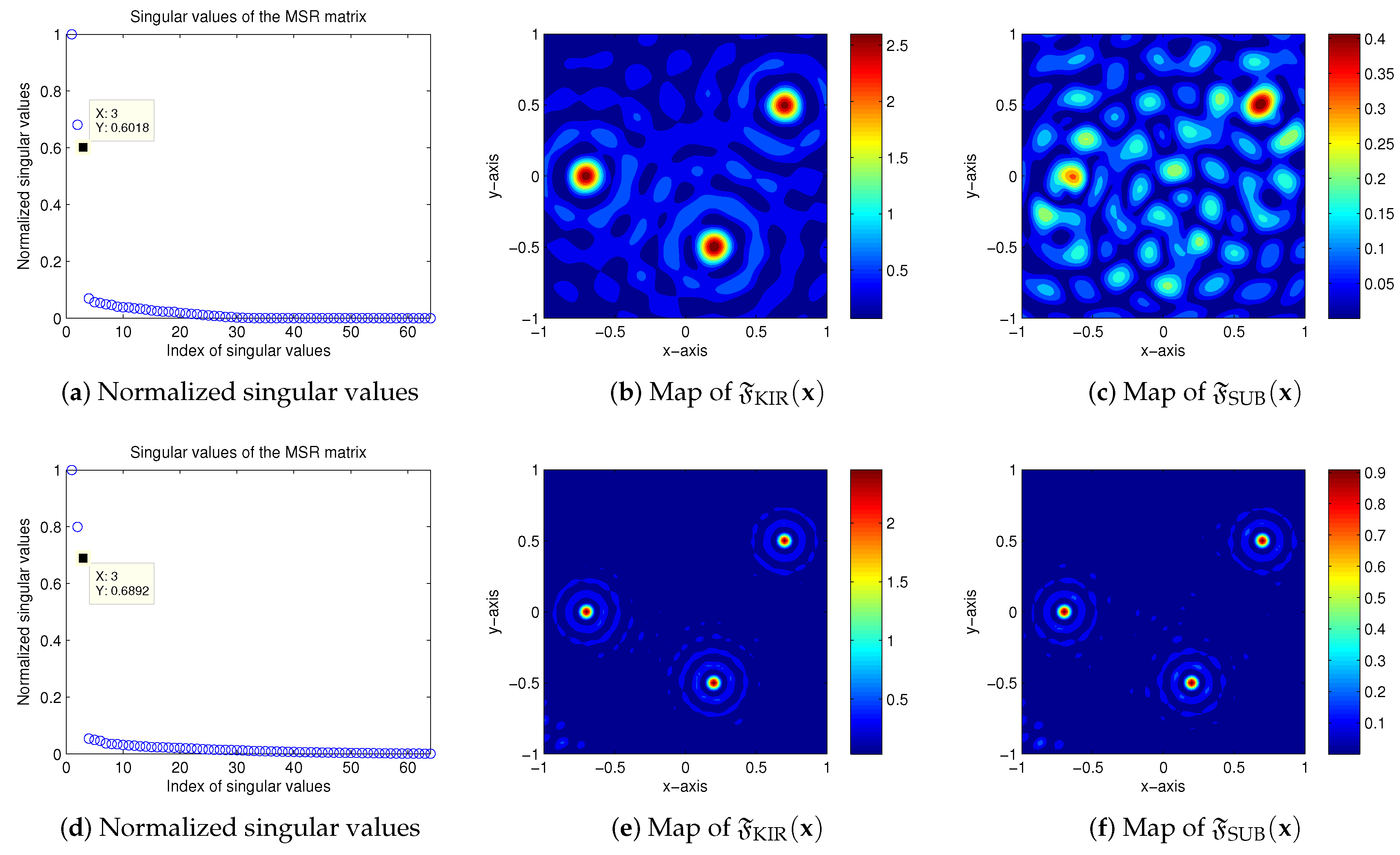
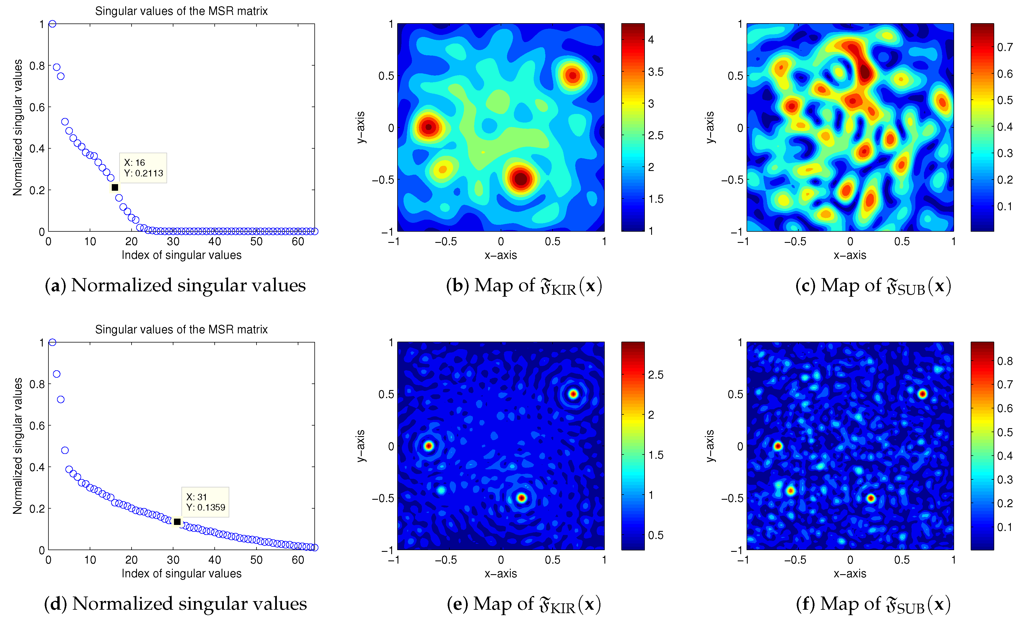
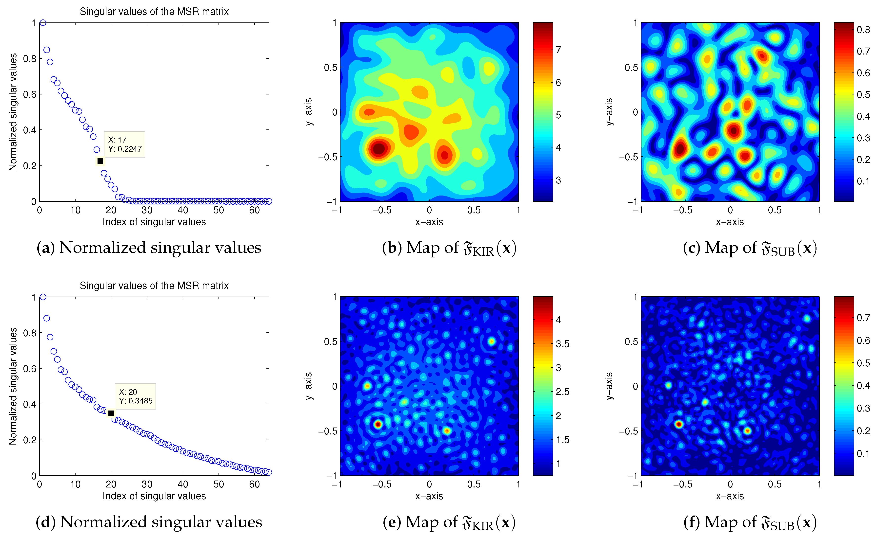
4. Simulation Results

In order to validate the results derived from Theorem 1, we now present a set of simulation results. In this section, we only consider the dielectric permittivity contrast case. For the simulation, $M=3$ small anomalies, all with the same permittivity ${\epsilon }_{\mathbf{A}}^{\left(m\right)}\equiv 5$, permeability ${\mu }_{\mathbf{A}}^{\left(m\right)}={\mu }_{\mathbf{R}}^{\left(s\right)}=1$, and radius ${\alpha }_m\equiv 0.1$ were placed at the following locations: ${\mathbf{x}}_{\mathrm{ANO}}^{\left(1\right)}={[0.25,0]}^T$, ${\mathbf{x}}_{\mathrm{ANO}}^{\left(2\right)}={[-0.4,0.5]}^T$, and ${\mathbf{x}}_{\mathrm{ANO}}^{\left(3\right)}={[-0.3,-0.7]}^T$. In addition, $S=100$ small scatterers were randomly distributed over $\mathsf{\Omega }=[-1,1]\times [-1,1]\subset {\mathbb{R}}^2$ such that

$${\mathbf{x}}_{\mathrm{RND}}^{\left(s\right)}={[{\eta }_1(-1,1),{\eta }_2(-1,1)]}^T,$$

where the ${\eta }_p(a,b)$, $p=1,2$, are arbitrary real values between a and b. Figure 1 shows the distribution of the three anomalies ${\mathbf{A}}_m$ and random scatterers ${\mathbf{R}}_s$. The data $u_{\infty }({\mathit{\vartheta }}_j,{\mathit{\theta }}_l)$ for the MSR matrix $\mathbb{K}$ was generated by solving the Foldy-Lax formulation to avoid an inverse crime (see [53] for instance). We used a total of $N=64$ incident and observation directions and wavelengths of $\lambda =0.7$ and $\lambda =0.2$ as low and high frequencies, respectively. After obtaining the far-field data, 20 dB Gaussian random noise is added to the unperturbed data through the MATLAB command awgn included in the signal processing package.

Example 1

(Case 1). In this Example, we consider the imaging results for examining Case 1. For this, we set the permittivities and radii of the random scatterers as ${\epsilon }_{\mathbf{R}}^{\left(s\right)}={\eta }_3(2,3)$ and ${\sigma }_s={\eta }_5(0.03,0.06)$. Figure 2 shows the distribution of $\mathbb{K}$’s normalized singular values and maps of ${\mathfrak{F}}_{\mathrm{SUB}}\left(\mathbf{x}\right)$ and ${\mathfrak{F}}_{\mathrm{KIR}}\left(\mathbf{x}\right)$ for both wavelengths. Note that although the 3 singular values were successfully discriminated, it is very hard to identify the anomaly locations from the ${\mathfrak{F}}_{\mathrm{SUB}}\left(\mathbf{x}\right)$ map for the low applied frequency ($\lambda =0.7$) due to the presence of huge numbers of artifacts. Fortunately, the three anomalies could be extracted satisfactorily from the ${\mathfrak{F}}_{\mathrm{KIR}}\left(\mathbf{x}\right)$ map at this frequency. At the higher frequency ($\lambda =0.2$), selecting the first 3 singular values allows the anomaly locations to be identified more clearly from the ${\mathfrak{F}}_{\mathrm{SUB}}\left(\mathbf{x}\right)$ map, supporting the discussion of Case 1. That said, the anomaly locations can also be extracted via Kirchhoff migration at this frequency.

Example 2

(Case 2). In this Example, we consider the imaging results for Case 2. For this, we set the permittivities and radii of the random scatterers as ${\epsilon }_{\mathbf{R}}^{\left(s\right)}={\eta }_6(3.5,4.5)$ and ${\sigma }_s={\eta }_8(0.05,0.1)$. Based on the Figure 3, it is far from clear that the first 3 singular values can be identified as the non-zero values of $\mathbb{K}$ so the exact threshold of the non-zero singular values cannot be determined. Hence, the ${\mathfrak{F}}_{\mathrm{SUB}}\left(\mathbf{x}\right)$ imaging results are poor at the lower frequency. Although there are some artifacts in the ${\mathfrak{F}}_{\mathrm{KIR}}\left(\mathbf{x}\right)$ map, all the anomaly locations can be accurately identified. In contrast, at the higher frequency, the ${\mathfrak{F}}_{\mathrm{SUB}}\left(\mathbf{x}\right)$ map allows all the anomaly locations to be retrieved very accurately although one random scatterer, located at ${[-0.58,-0.42]}^T$, is also identified. The permittivity and radius of this random scatterer were $2.5596$ and $0.0998$, respectively. This scatterer’s location was also identified by the ${\mathfrak{F}}_{\mathrm{KIR}}\left(\mathbf{x}\right)$ map, but its magnitude was small enough that the anomaly locations could still be accurately identified via Kirchhoff migration.

Example 3

(Selection of nonzero singular values: Cases 1 and 2). Figure 4 exhibits maps of ${\mathfrak{F}}_{\mathrm{SUB}}\left(\mathbf{x}\right)$ with various selection of nonzero singular values $N_0$. By regarding the distribution of normalized singular values of $\mathbb{K}$ in Figure 3d, the number $N_0$ are chosen as 3, 4, and 15 for evaluating ${\mathfrak{F}}_{\mathrm{SUB}}\left(\mathbf{x}\right)$. Notice that if one selects $N_0=3$, which is the same number of anomalies ${\mathbf{A}}_m$, it is possible to obtain a good result. Furthermore, by comparing with the Figure 3e, this result is better than the one via the map of ${\mathfrak{F}}_{\mathrm{KIR}}\left(\mathbf{x}\right)$ so that subspace migration will provide better results to the Kirchhoff migration when appropriate number of singular values are chosen. In contrast, if $N_0=4$ is chosen, Kirchhoff migration provides better results than subspace migration because the location of one random scatterer, located at ${[-0.58,-0.42]}^T$, is retrieved clearly in the map of ${\mathfrak{F}}_{\mathrm{SUB}}\left(\mathbf{x}\right)$. If one selects $N_0=15$, similar to the Figure 3e, the map of ${\mathfrak{F}}_{\mathrm{SUB}}\left(\mathbf{x}\right)$ provides locations of anomalies, single random scatterer, and unexpected artifacts. This result supports the discussions in Cases 1 and 2.

Example 4

(Case 3). In this Example, we consider the imaging results for Case 3. For this, we set the permittivities and radii of the random scatterers as ${\epsilon }_{\mathbf{R}}^{\left(s\right)}={\eta }_9(4,5)$, ${\epsilon }_{\mathbf{R}}^{\left(s\right)}={\eta }_{10}(4,5)$, and ${\sigma }_s={\eta }_{11}(0.07,0.14)$, respectively. In this case, there was no relationship between ${\alpha }_m$ and ${\sigma }_s$, ${\epsilon }_{\mathbf{A}}^{\left(m\right)}$ and ${\epsilon }_{\mathbf{R}}^{\left(s\right)}$, or ${\mu }_{\mathbf{A}}^{\left(m\right)}$ and ${\mu }_{\mathbf{R}}^{\left(s\right)}$ for any m and s, so it was impossible to distinguish locations of the anomalies and random scatterers accurately via subspace or Kirchhoff migration at either the low or high frequency, as shown in the Figure 5.

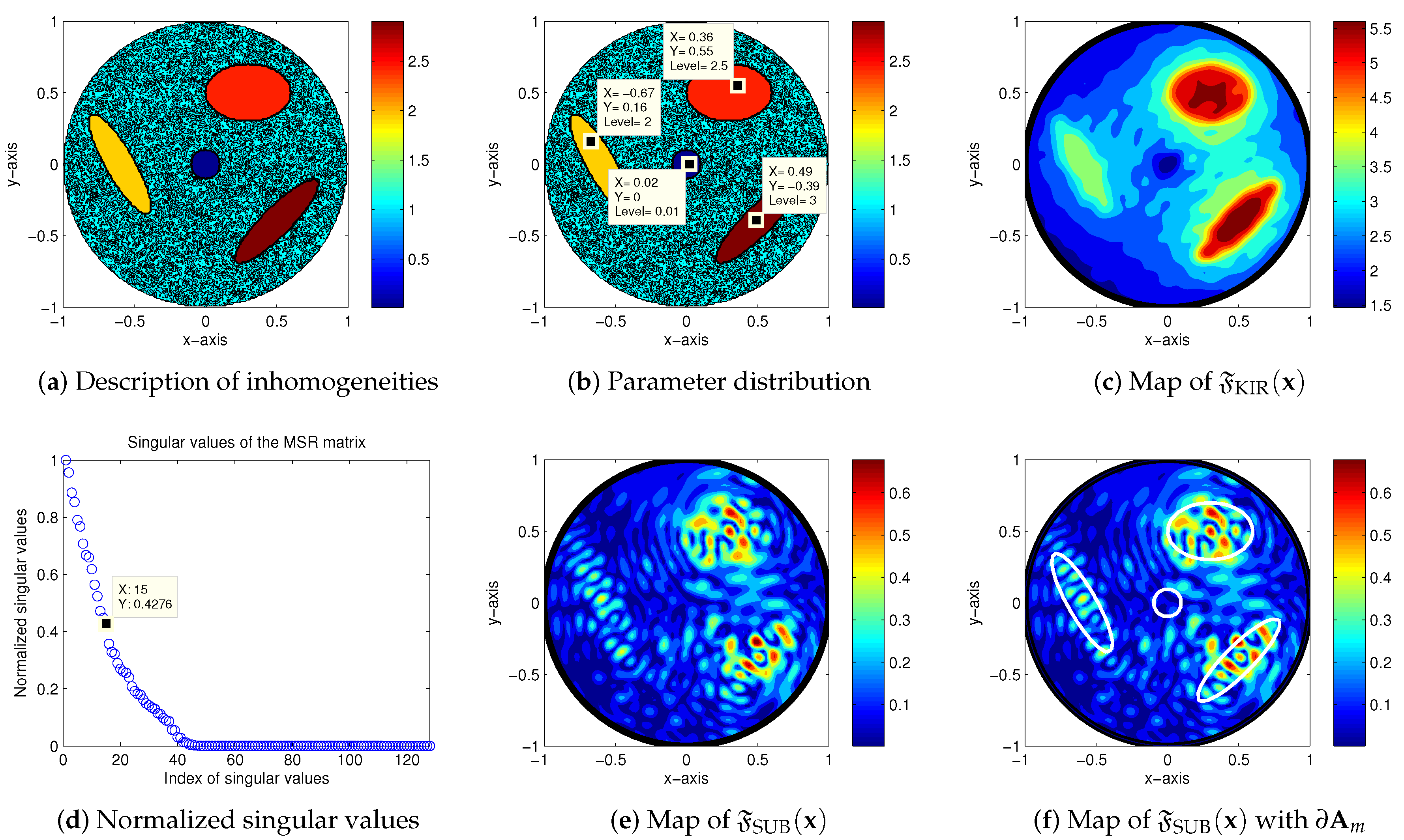
5. Further Result: Imaging of Extended Dielectric Targets in an Inhomogeneous Medium

To examine the effectiveness of Kirchhoff migration, additional numerical simulation about the imaging of extended targets completely embedded in an inhomogeneous medium were performed. Following the test configuration in [54], we consider only the permittivity contrast case and set the inhomogeneous domain $\mathsf{\Omega }$ to be a unit circle with a permittivity of ${\epsilon }_0=\eta (0.5,1.5)$. For the sake, we set the value of permeability $\mu \left(\mathbf{x}\right)={\mu }_0\equiv 1$ for $\mathbf{x}\in \mathsf{\Omega }$. We assumed the existence of four extended inhomogeneities ${\mathbf{A}}_m\subset \mathsf{\Omega }$ with smooth boundaries $\partial {\mathbf{A}}_m$ satisfying $\partial {\mathbf{A}}_m\cap \partial \mathsf{\Omega }=⌀$ and permittivities ${\epsilon }_m$, $m=1,2,3,4$. The shapes of ${\mathbf{A}}_m$ are shown in the Figure 6, and their boundaries are expressed as

$$\begin{array}{cc}\partial {\mathbf{A}}_1=\left\{[s,t]:11.11{(s-0.3)}^2+25{(t-0.5)}^2=1\right\},\hfill & {\epsilon }_1=2.5\hfill \\ \partial {\mathbf{A}}_2=\left\{[s,t]:53.1250{(s-0.5)}^2-93.75(s-0.5)(t+0.4)+53.1250{(t+0.4)}^2=1\right\},\hfill & {\epsilon }_2=3\hfill \\ \partial {\mathbf{A}}_3=\left\{[s,t]:76.5625{(s+0.6)}^2+81.1898(s+0.6)t+29.6875t^2=1\right\},\hfill & {\epsilon }_3=2\hfill \\ \partial {\mathbf{A}}_4=\left\{[s,t]:s^2+t^2=0.01\right\},\hfill & {\epsilon }_4=0.01.\hfill \end{array}$$

With this configuration, we denote the time-harmonic total field as $u^{\left(n\right)}\left(\mathbf{x}\right)$, which satisfies the following boundary value problem

$$\left\{\begin{array}{ccc}\hfill \Delta u^{\left(n\right)}\left(\mathbf{x}\right)+{\omega }^2\epsilon \left(\mathbf{x}\right)u^{\left(n\right)}\left(\mathbf{x}\right)=0& \mathrm{in}& \mathsf{\Omega }\hfill \\ \hfill {\displaystyle \frac{\partial u^{\left(n\right)}\left(\mathbf{x}\right)}{\partial \nu \left(\mathbf{x}\right)}=\frac{\partial e^{ik{\mathit{\theta }}_n·\mathbf{x}}}{\partial \nu \left(\mathbf{x}\right)}}& \mathrm{on}& \partial \mathsf{\Omega }\hfill \end{array}\right.$$

(8)

and with transmission condition on the boundary $\partial {\mathbf{A}}_m$, $m=1,2,3,4$. Here, $\nu \left(\mathbf{x}\right)$ is the unit normal to $\partial \mathsf{\Omega }$ at $\mathbf{x}$, and ${\mathit{\theta }}_n$, $n=1,2,\cdots ,N(=128)$ denotes a two-dimensional vector on the $\partial \mathsf{\Omega }$, such that

$${\mathit{\theta }}_n={\left[cos\frac{2\pi n}{N},sin\frac{2\pi n}{N}\right]}^T.$$

Similarly, $u_0^{\left(n\right)}\left(\mathbf{x}\right)=e^{ik{\mathit{\theta }}_n·\mathbf{x}}$ denotes the solution of (8) without anomalies and constant ${\epsilon }_0\equiv 1$.

Based on [12,51], $u^{\left(n\right)}\left(\mathbf{x}\right)-u_0^{\left(n\right)}\left(\mathbf{x}\right)$ can be represented as

$$u^{\left(n\right)}\left(\mathbf{x}\right)-u_0^{\left(n\right)}\left(\mathbf{x}\right)=\sum _{m=1}^4{\int }_{\partial {\mathbf{A}}_m}\mathcal{N}(\mathbf{x},\mathbf{y}){\varphi }^{\left(n\right)}\left(\mathbf{y}\right)d\mathbf{y}+\mathcal{E}\left({\epsilon }_0\right),$$

(9)

where ${\varphi }^{\left(n\right)}\left(\mathbf{y}\right)$ is an unknown density function, $\mathcal{E}\left({\epsilon }_0\right)$ denotes an error term that is highly depending on the value of ${\epsilon }_0$, and $\mathcal{N}(\mathbf{x},\mathbf{y})$ satisfies

$$\left\{\begin{array}{ccc}\hfill \Delta \mathcal{N}(\mathbf{x},\mathbf{y})+k^2\mathcal{N}(\mathbf{x},\mathbf{y})=-\delta (\mathbf{x},\mathbf{y})& \mathrm{in}& \mathsf{\Omega }\hfill \\ \hfill {\displaystyle \frac{\partial \mathcal{N}(\mathbf{x},\mathbf{y})}{\partial \nu \left(\mathbf{y}\right)}=0}& \mathrm{on}& \partial \mathsf{\Omega }.\hfill \end{array}\right.$$

Here, $\delta$ denotes the dirac delta function. On the basis of (9), we cannot use the boundary measurement data $u^{\left(n\right)}\left(\mathbf{x}\right)-u_0^{\left(n\right)}\left(\mathbf{x}\right)$ directly to design the Kirchhoff and subspace migrations. So, motivated by [12], we consider the following normalized boundary measurement data ${\mathrm{B}}_{\mathrm{meas}}(n,n^{\prime })$

$${\mathrm{B}}_{\mathrm{meas}}(n,n^{\prime }):={\int }_{\partial \mathsf{\Omega }}\left(u^{\left(n\right)}\left(\mathbf{x}\right)-u_0^{\left(n\right)}\left(\mathbf{x}\right)\right)\frac{\partial v^{\left(n^{\prime }\right)}\left(\mathbf{x}\right)}{\partial \nu \left(\mathbf{x}\right)}dS\left(\mathbf{x}\right)=\sum _{m=1}^4{\int }_{\partial {\mathbf{A}}_m}{e}^{-ik{\mathit{\theta }}_{n^{\prime }}·\mathbf{y}}{\varphi }^{\left(n\right)}\left(\mathbf{y}\right)d\mathbf{y}+\mathcal{E}\left({\epsilon }_0\right),$$

(10)

where $v^{\left(n^{\prime }\right)}\left(\mathbf{x}\right)=e^{-ik{\mathit{\theta }}_{n^{\prime }}·\mathbf{x}}$.

Now, let us consider the following MSR matrix

$$\mathbb{K}=\left[\begin{array}{cccc}{\mathrm{B}}_{\mathrm{meas}}(1,1)& {\mathrm{B}}_{\mathrm{meas}}(1,2)& \cdots & {\mathrm{B}}_{\mathrm{meas}}(1,N)\\ {\mathrm{B}}_{\mathrm{meas}}(2,1)& {\mathrm{B}}_{\mathrm{meas}}(2,2)& \cdots & {\mathrm{B}}_{\mathrm{meas}}(2,N)\\ ⋮& ⋮& \ddots & ⋮\\ {\mathrm{B}}_{\mathrm{meas}}(N,1)& {\mathrm{B}}_{\mathrm{meas}}(N,2)& \cdots & {\mathrm{B}}_{\mathrm{meas}}(N,N)\end{array}\right].$$

Then, $\mathbb{K}$ can be decomposed as (see [14] for instance)

$$\mathbb{K}\approx \sum _{m=1}^4{\int }_{\partial {\mathbf{A}}_m}\mathbb{E}\left(\mathbf{y}\right)\mathbb{D}\left(\mathbf{y}\right)d\mathbf{y},$$

where $\mathbb{E}\left(\mathbf{y}\right)$ and $\mathbb{D}\left(\mathbf{y}\right)$ denote the illumination and resulting density vectors

$$\mathbb{E}\left(\mathbf{y}\right)={\left[e^{-ik{\mathit{\theta }}_1·\mathbf{y}},e^{-ik{\mathit{\theta }}_2·\mathbf{y}},\cdots ,e^{-ik{\mathit{\theta }}_N·\mathbf{y}}\right]}^T\mathrm{and}\mathbb{D}\left(\mathbf{y}\right)=\left[{\varphi }^{\left(1\right)}\left(\mathbf{y}\right),{\varphi }^{\left(2\right)}\left(\mathbf{y}\right),\cdots ,{\varphi }^{\left(N\right)}\left(\mathbf{y}\right)\right],$$

(11)

respectively.

Based on [14], it should be noted that the range of $\mathbb{K}$ is determined by the span of the $\mathbb{E}\left(\mathbf{y}\right)$ corresponding to ${\mathbf{A}}_m$. This means that the signal subspace can be determined by selecting the singular vectors associated with the nonzero singular values of $\mathbb{K}$. Thus, by taking the test vector $\mathbf{W}\left(\mathbf{x}\right)$ of (5) as

$$\mathbf{W}\left(\mathbf{x}\right)=\frac{1}{\sqrt{N}}{\left[e^{-ik{\mathit{\theta }}_1·\mathbf{x}},e^{-ik{\mathit{\theta }}_2·\mathbf{x}},\cdots ,e^{-ik{\mathit{\theta }}_N·\mathbf{x}}\right]}^T,$$

imaging functions ${\mathfrak{F}}_{\mathrm{KIR}}\left(\mathbf{x}\right)$ and ${\mathfrak{F}}_{\mathrm{SUB}}\left(\mathbf{x}\right)$ can be defined similarly with (4) and (7), respectively.

Example 5

(Imaging performances of Kirchhoff and subspace migrations). Figure 6 shows the imaging results via ${\mathfrak{F}}_{\mathrm{KIR}}\left(\mathbf{x}\right)$ and ${\mathfrak{F}}_{\mathrm{SUB}}\left(\mathbf{x}\right)$ when $\lambda =0.3$. We also mention that 20dB Gaussian random noise is added to the unperturbed data ${\mathrm{B}}_{\mathrm{meas}}(n,n^{\prime })$, $n,n^{\prime }=1,2,\cdots ,N$. For performing subspace migration, first 15 singular values are selected. In contrast to the traditional results, it is very hard to identify the outline shapes of every inhomogeneity via ${\mathfrak{F}}_{\mathrm{SUB}}\left(\mathbf{x}\right)$ while it is possible to identify the outline shape of every inhomogeneity. Although the size and permittivity of ${\mathbf{A}}_4$ were both very small, the existence of ${\mathbf{A}}_4$ was successfully recognized. On the basis of simulation results, we conclude that the result via Kirchhoff migration is better than the one via subspace migration for addressing problems of this type.

Example 6

(Influence of total number of incident fields). Based on the condition in Theorem 1, let us examine the effect of total number N of incident fields. Figure 7 exhibits the maps of ${\mathfrak{F}}_{\mathrm{KIR}}\left(\mathbf{x}\right)$ and ${\mathfrak{F}}_{\mathrm{SUB}}\left(\mathbf{x}\right)$ for $N=32$ and 64. Similar to the traditional researches, it appears that small value of N might be a reason of poor result while large value of N will guarantee good imaging performance of Kirchhoff migration. Unfortunately, it is impossible to identify outline shape of all ${\mathbf{A}}_m$ through the subspace migration with small and large N.

Example 7

(Comparison of imaging performances). For the final example, let us apply various non-iterative techniques such as MUSIC, direct sampling method, and factorization method for imaging extended targets and compare the imaging performances. In Figure 8, imaging results via subspace migration (map of ${\mathfrak{F}}_{\mathrm{SUB}}\left(\mathbf{x}\right)$), MUSIC (map of ${\mathfrak{F}}_{\mathrm{MUSIC}}\left(\mathbf{x}\right)$), direct sampling method (map of ${\mathfrak{F}}_{\mathrm{DSM}}\left(\mathbf{x}\right)$), and factorization method (map of ${\mathfrak{F}}_{\mathrm{FM}}\left(\mathbf{x}\right)$) are exhibited with the same simulation configuration of Figure 6.

First, let us compare the imaging results via subspace migration and MUSIC algorithm with different selection of nonzero singular values. For this, different from the Figure 6e, $N_0=10$ and $N_0=37$ nonzero singular values are selected to define ${\mathfrak{F}}_{\mathrm{SUB}}\left(\mathbf{x}\right)$. However, for any selection of $N_0$, an outline shape of inhomogeneities ${\mathbf{A}}_m$ cannot be retrieved. Thus, we can examine that the result via Kirchhoff migration is better than the one via subspace migration and MUSIC for imaging of arbitrary shaped inhomogeneities embedded in a random medium.

Next, let us consider the imaging result via direct sampling method with a fixed incident direction ${\mathit{\theta }}_1$. Based on the Figure 8c, we can easily examine that the result via direct sampling method is poorer than the one via Kirchhoff migration. Notice that Kirchhoff migration and direct sampling method are identical when the number of incident fields becomes sufficiently large (see Section 5, [24]) so that total number of incident fields must be large enough to obtain a good result via direct sampling method.

Figure 8c shows the imaging result via factorization method. It is interesting to observe that similar to the imaging result via Kirchhoff migration, the outline shapes of inhomogeneities are also successfully retrieved. Hence, factorization method can be regarded as an appropriate imaging technique in random medium.

6. Conclusions

In this paper, we have considered Kirchhoff migration techniques for locating small anomalies when they are surrounded by small random scatterers. In order to investigate the mathematical structure of imaging function and examine the imaging performance, we carefully established a relationship with Bessel functions of the first kind of order zero and one based on the asymptotic expansion formula in the presence of anomalies and random scatterers. Based on the established relationship, we showed that Kirchhoff migration can be regarded as an effective non-iterative technique for identifying the locations of small anomalies when the sizes and permittivities of the random scatterers are smaller than those of the anomalies and the applied frequency is high enough. However, when one of these conditions is not satisfied, the imaging results are somehow poor but Kirchhoff migration yields better results than various non-iterative techniques such as subspace migration, MUSIC, direct sampling method, etc. We have also presented simulation results for several different cases to validate these relationships and observed properties. Although we have discovered various properties of Kirchhoff migration, some phenomenon cannot yet be explained. Further development of mathematical theory for explaining such phenomenon will be a remarkable research topic. Here, we considered the two-dimensional problem, the analysis could be extended to the three-dimensional problem.

References

1. Ammari, H. An Introduction to Mathematics of Emerging Biomedical Imaging; Mathematics and Applications Series; Springer: Berlin, Germany, 2008; Volume 62. [Google Scholar]
2. Arridge, S. Optical tomography in medical imaging. Inverse Probl. 1999, 15, R41–R93. [Google Scholar] [CrossRef] [Green Version]
3. Colton, D.; Piana, M.; Potthast, R. A simple method using Morozov’s discrepancy principle for solving inverse scattering problems. Inverse Probl. 2017, 13, 1477–1493. [Google Scholar] [CrossRef]
4. Haynes, M.; Stang, J.; Moghaddam, M. Real-time microwave imaging of differential temperature for thermal therapy monitoring. IEEE Trans. Biomed. Eng. 2014, 61, 1787–1797. [Google Scholar] [CrossRef] [PubMed]
5. Irishina, N.; Dorn, O.; Moscoso, M. A level set evolution strategy in microwave imaging for early breast cancer detection. Comput. Math. Appl. 2008, 56, 607–618. [Google Scholar] [CrossRef] [Green Version]
6. Kim, Y.J.; Jofre, L.; Flaviis, F.D.; Feng, M.Q. Microwave reflection tomographic array for damage detection of civil structures. IEEE Trans. Antennas Propag. 2003, 51, 3022–3032. [Google Scholar]
7. Kim, C.K.; Lee, J.S.; Chae, J.S.; Park, S.O. A modified stripmap SAR processing for vector velocity compensation using the cross-correlation estimation method. J. Electromagn. Eng. Sci. 2019, 19, 159–165. [Google Scholar] [CrossRef]
8. Meaney, P.M.; Fanning, M.W.; Li, D.; Poplack, S.P.; Paulsen, K.D. A clinical prototype for active microwave imaging of the breast. IEEE Trans. Microwave Theory Tech. 2000, 48, 1841–1853. [Google Scholar]
9. Shea, J.D.; Kosmas, P.; Veen, B.D.V.; Hagness, S.C. Contrast-enhanced microwave imaging of breast tumors: A computational study using 3-D realistic numerical phantoms. Inverse Probl. 2010, 26, 074009. [Google Scholar] [CrossRef]
10. Seo, T.; Oh, S.; Jung, D.; Huh, Y.; Cho, J.; Kwon, Y. Noninvasive brain stimulation using a modulated microwave signal. J. Electromagn. Eng. Sci. 2018, 18, 70–72. [Google Scholar] [CrossRef]
11. Ammari, H.; Iakovleva, E.; Lesselier, D. A MUSIC algorithm for locating small inclusions buried in a half-space from the scattering amplitude at a fixed frequency. Multiscale Model. Simul. 2005, 3, 597–628. [Google Scholar] [CrossRef]
12. Ammari, H.; Kang, H.; Lee, H.; Park, W.K. Asymptotic imaging of perfectly conducting cracks. SIAM J. Sci. Comput. 2010, 32, 894–922. [Google Scholar] [CrossRef]
13. Chen, X.; Zhong, Y. MUSIC electromagnetic imaging with enhanced resolution for small inclusions. Inverse Probl. 2009, 25, 015008. [Google Scholar] [CrossRef]
14. Hou, S.; Sølna, K.; Zhao, H. A direct imaging algorithm for extended targets. Inverse Probl. 2006, 22, 1151–1178. [Google Scholar] [CrossRef]
15. Park, W.K. Asymptotic properties of MUSIC-type imaging in two-dimensional inverse scattering from thin electromagnetic inclusions. SIAM J. Appl. Math. 2015, 75, 209–228. [Google Scholar] [CrossRef]
16. Cheney, M. The linear sampling method and the MUSIC algorithm. Inverse Probl. 2001, 17, 591–595. [Google Scholar] [CrossRef] [Green Version]
17. Cakoni, F.; Colton, D. The linear sampling method for cracks. Inverse Probl. 2003, 19, 279–295. [Google Scholar] [CrossRef]
18. Colton, D.; Haddar, H.; Monk, P. The linear sampling method for solving the electromagnetic inverse scattering problem. SIAM J. Sci. Comput. 2002, 24, 719–731. [Google Scholar] [CrossRef]
19. Colton, D.; Haddar, H.; Piana, M. The linear sampling method in inverse electromagnetic scattering theory. Inverse Probl. 2003, 19, S105–S137. [Google Scholar] [CrossRef]
20. Haddar, H.; Monk, P. The linear sampling method for solving the electromagnetic inverse medium problem. Inverse Probl. 2002, 18, 891–906. [Google Scholar] [CrossRef]
21. Kirsch, A.; Ritter, S. A linear sampling method for inverse scattering from an open arc. Inverse Probl. 2000, 16, 89–105. [Google Scholar] [CrossRef]
22. Ito, K.; Jin, B.; Zou, J. A direct sampling method to an inverse medium scattering problem. Inverse Probl. 2012, 28, 025003. [Google Scholar] [CrossRef]
23. Li, J.; Zou, J. A direct sampling method for inverse scattering using far-field data. Inverse Probl. Imag. 2013, 7, 757–775. [Google Scholar] [CrossRef]
24. Kang, S.; Lambert, M.; Park, W.K. Direct sampling method for imaging small dielectric inhomogeneities: Analysis and improvement. Inverse Probl. 2018, 34, 095005. [Google Scholar] [CrossRef]
25. Park, W.K. Detection of small inhomogeneities via direct sampling method in transverse electric polarization. Appl. Math. Lett. 2018, 79, 169–175. [Google Scholar] [CrossRef] [Green Version]
26. Park, W.K. Direct sampling method for retrieving small perfectly conducting cracks. J. Comput. Phys. 2018, 373, 648–661. [Google Scholar] [CrossRef] [Green Version]
27. Ammari, H.; Garnier, J.; Jugnon, V.; Kang, H. Stability and resolution analysis for a topological derivative based imaging functional. SIAM J. Control Optim. 2012, 50, 48–76. [Google Scholar] [CrossRef]
28. Guzina, B.; Pourahmadian, F. Why the high-frequency inverse scattering by topological sensitivity may work. Proc. R. Soc. A 2015, 471, 20150187. [Google Scholar] [CrossRef] [Green Version]
29. Park, W.K. Multi-frequency topological derivative for approximate shape acquisition of curve-like thin electromagnetic inhomogeneities. J. Math. Anal. Appl. 2013, 404, 501–518. [Google Scholar] [CrossRef] [Green Version]
30. Park, W.K. Topological derivative strategy for one-step iteration imaging of arbitrary shaped thin, curve-like electromagnetic inclusions. J. Comput. Phys. 2012, 231, 1426–1439. [Google Scholar] [CrossRef]
31. Park, W.K. Performance analysis of multi-frequency topological derivative for reconstructing perfectly conducting cracks. J. Comput. Phys. 2017, 335, 865–884. [Google Scholar] [CrossRef] [Green Version]
32. Ammari, H.; Iakovleva, E.; Moskow, S. Recovery of small inhomogeneities from the scattering amplitude at a fixed frequency. SIAM J. Math. Anal. 2003, 34, 882–900. [Google Scholar] [CrossRef]
33. Ammari, H.; Moskow, S.; Vogelius, M. Boundary integral formulas for the reconstruction of electromagnetic imperfections of small diameter. ESAIM Control Optim. Calc. Var. 2003, 9, 49–66. [Google Scholar] [CrossRef]
34. Chapko, R.; Kress, R. A hybrid method for inverse boundary values problems in potential theory. J. Inverse Ill Posed Probl. 2005, 13, 1–14. [Google Scholar] [CrossRef]
35. Colton, D.; Kirsch, A. A simple method for solving inverse scattering problems in the resonance region. Inverse Probl. 1996, 12, 383–393. [Google Scholar] [CrossRef]
36. Salucci, M.; Anselmi, N.; Oliveri, G.; Calmon, P.; Miorelli, R.; Reboud, C.; Massa, A. Real-time NDT-NDE through an innovative adaptive partial least squares SVR inversion approach. IEEE Trans. Geosci. Remote Sens. 2016, 54, 6818–6832. [Google Scholar] [CrossRef]
37. Salucci, M.; Vrba, J.; Merunka, I.; Massa, A. Real-time brain stroke detection through a learning-by-examples technique—An experimental assessment. Microw. Opt. Technol. Lett. 2017, 59, 2796–2799. [Google Scholar] [CrossRef]
38. Ammari, H.; Garnier, J.; Kang, H.; Park, W.K.; Sølna, K. Imaging schemes for perfectly conducting cracks. SIAM J. Appl. Math. 2011, 71, 68–91. [Google Scholar] [CrossRef]
39. Bleistein, N.; Cohen, J.; Stockwell, J.S., Jr. Mathematics of Multidimensional Seismic Imaging, Migration, and Inversion; Springer: New York, NY, USA, 2001. [Google Scholar]
40. Joh, Y.D.; Park, W.K. Analysis of multi-frequency subspace migration weighted by natural logarithmic function for fast imaging of two-dimensional thin, arc-like electromagnetic inhomogeneities. Comput. Math. Appl. 2014, 68, 1892–1904. [Google Scholar] [CrossRef] [Green Version]
41. Park, W.K. Multi-frequency subspace migration for imaging of perfectly conducting, arc-like cracks in full- and limited-view inverse scattering problems. J. Comput. Phys. 2015, 283, 52–80. [Google Scholar] [CrossRef] [Green Version]
42. Park, W.K. A novel study on subspace migration for imaging of a sound-hard arc. Comput. Math. Appl. 2017, 74, 3000–3007. [Google Scholar] [CrossRef]
43. Park, W.K. Real-time microwave imaging of unknown anomalies via scattering matrix. Mech. Syst. Signal Proc. 2019, 118, 658–674. [Google Scholar] [CrossRef]
44. Borcea, L.; Papanicolaou, G.; Tsogka, C.; Berryman, J. Imaging and time reversal in random media. Inverse Probl. 2002, 18, 1247–1279. [Google Scholar] [CrossRef] [Green Version]
45. Chen, B.; Stamnes, J.J.; Devaney, A.J.; Pedersen, H.M.; Stamnes, K. Two-dimensional optical diffraction tomography for objects embedded in a random medium. Pure Appl. Opt. J. Eur. Opt. Soc. Part A 1998, 7, 1181. [Google Scholar] [CrossRef]
46. Kirsch, A. The MUSIC algorithm and the factorization method in inverse scattering theory for inhomogeneous media. Inverse Probl. 2002, 18, 1025–1040. [Google Scholar] [CrossRef]
47. Shevtsov, B.M. Backscattering and inverse problem in random media. J. Math. Phys. 1999, 40, 4359–4373. [Google Scholar] [CrossRef]
48. Park, W.K. Interpretation of MUSIC for location detecting of small inhomogeneities surrounded by random scatterers. Math. Probl. Eng. 2016, 2016, 7872548. [Google Scholar] [CrossRef]
49. Park, W.K.; Lesselier, D. Fast electromagnetic imaging of thin inclusions in half-space affected by random scatterers. Waves Random Complex Media 2012, 22, 3–23. [Google Scholar] [CrossRef]
50. Ammari, H.; Garnier, J.; Sølna, K. A statistical approach to target detection and localization in the presence of noise. Waves Random Complex Media 2012, 22, 40–65. [Google Scholar] [CrossRef]
51. Ammari, H.; Kang, H. Reconstruction of Small Inhomogeneities from Boundary Measurements; Lecture Notes in Mathematics; Springer: Berlin, Germany, 2004; Volume 1846. [Google Scholar]
52. Park, W.K. Detection of small electromagnetic inhomogeneities with inaccurate frequency. J. Korean Phys. Soc. 2016, 68, 607–615. [Google Scholar] [CrossRef] [Green Version]
53. Huang, K.; Sølna, K.; Zhao, H. Generalized Foldy-Lax formulation. J. Comput. Phys. 2010, 229, 4544–4553. [Google Scholar] [CrossRef] [Green Version]
54. Ahn, C.Y.; Ha, T.; Jeon, K.; Park, W.K. Application of MUSIC for shape identification of dielectric extended targets in inhomogeneous medium. In Proceeding of Progress in Electromagnetics Research Symposium, Shanghai, China, 8–11 August 2016; pp. 3002–3006. [Google Scholar]
Figure 1. Distribution of anomalies A m (red dots) and random scatterers R s (blue ‘×’ symbols).
Applsci 09 04446 g001
Figure 2. (Example 1: Case 1) Distribution of normalized singular values, maps of F KIR ( x ) and F SUB ( x ) for λ = 0.7 (top line) and λ = 0.2 (bottom line).
Applsci 09 04446 g002
Figure 3. (Example 2: Case 2) Distribution of normalized singular values, maps of F KIR ( x ) and F SUB ( x ) for λ = 0.7 (top line) and λ = 0.2 (bottom line).
Applsci 09 04446 g003
Figure 4. (Example 3: Case 2) Maps of F SUB ( x ) for λ = 0.2 .
Applsci 09 04446 g004
Figure 5. (Example 4: Case 3) Distribution of normalized singular values, maps of F KIR ( x ) and F SUB ( x ) for λ = 0.7 (top line) and λ = 0.2 (bottom line).
Applsci 09 04446 g005
Figure 6. (Example 5) Imaging results for extended targets embedded in an inhomogeneous medium.
Applsci 09 04446 g006
Figure 7. (Example 6) Distribution of normalized singular values, maps of F KIR ( x ) and F SUB ( x ) for λ = 0.3 with N = 32 directions (top line) and N = 64 directions (bottom line).
Applsci 09 04446 g007
Figure 8. (Example 7) Imaging results via the subspace migration, MUSIC, direct sampling method, and factorization method for λ = 0.3 with N = 128 .
Applsci 09 04446 g008