Deep Neural Network for Ore Production and Crusher Utilization Prediction of Truck Haulage System in Underground Mine

Abstract

A new method using a deep neural network (DNN) model is proposed to predict the ore production and crusher utilization of a truck haulage system in an underground mine. An underground limestone mine was selected as the study area, and the DNN model input/output nodes were designed to reflect the truck haulage system characteristics. Big data collected on-site for 1 month were processed to create learning datasets. To select the optimal DNN learning model, the numbers of hidden layers and hidden layer nodes were set to various values for analyzing the training and test data. The optimal DNN model structure for ore production prediction was set to five hidden layers and 40 hidden layer nodes. The test data exhibited a coefficient of determination of 0.99 and mean absolute percentage error (MAPE) of 2.80%. The optimal configuration for the crusher utilization prediction was set to four hidden layers and 40 hidden layer nodes, and the test data exhibited a coefficient of determination of 0.99 and MAPE of 2.49%. The trained DNN model was used to predict the ore production and crusher utilization, which were similar to the actual observed values.

1. Introduction

The design and operation of haulage systems are very important in mining sites. This is because mining costs may vary significantly according to the design and operation methods [1]. Various simulation techniques have been used for haulage systems in mines [2,3,4,5,6,7,8]. In the case of a mine truck haulage system, simulations may be used to predict productivity indices, such as the mine production and equipment utilization, according to system operating conditions, including the task time, amount of equipment, dispatch interval, and time consumed per unit task [9,10]. In this manner, it is possible to select optimal equipment combinations [11,12,13,14], establish equipment dispatch plans [10,15,16,17,18], and identify optimal haulage routes [19,20,21,22].

The numerous simulation techniques that have been developed thus far are based on algorithms that consider the sequential tasks performed by trucks. However, algorithm-based simulation techniques have certain problems. Mines are dynamic systems and hence unexpected events often occur, such as failure of mining equipment and crusher capacity overflow. Accurate simulations require humans to design and develop haulage system logic, taking into account all events that may occur in a mining environment. In addition, it is necessary to modify existing algorithms to consider a new loading point or haulage road changes and several algorithms should be adapted to simulate real-time dispatching truck haulage systems.

To address these problems, technologies such as sensor networks, mobile devices, the Internet of things, and cloud computing have been introduced into mining sites, and researchers have been studying simulation techniques using big data collected on-site rather than algorithms based on prior knowledge [23]. Moreover, deep learning has been attracting attention as a technology that efficiently analyzes big data according to its purpose [24,25]. Deep learning is an artificial intelligence technology that learns object characteristics hierarchically, without human interference, and improves the prediction performance by means of error evaluation [26]. Deep learning was developed based on the deep neural network (DNN), which is a supervised machine-learning technique [27]. DNNs imitate the neurons (nodes) and synapses that connect the neurons within the human brain. They have a multilayer perceptron structure in which an input layer, output layer, and one or more hidden layers are connected hierarchically [28,29,30]. The nodes of each layer are connected to all nodes on the next layer, and the output values are determined through a feed-forward network [31].

Various deep learning models based on the DNN have been developed by numerous researchers [32]. Convolutional neural networks (CNNs) are used to learn two-dimensional pixel data, such as images and videos [33]. A CNN is composed of a convolutional layer, pooling layer, and fully connected layer. It calculates the sum of weights between the training data and filter (or kernel) to extract detailed characteristics from images [34]. A recurrent neural network (RNN) is a model suitable for learning time series data that change sequentially over time [35]. It is mainly used to save the input elements of the previous time stage in the neural network and to predict the value of the next time stage [36]. Furthermore, auto-encoders are models that continuously perform encoding and decoding tasks to analyze the characteristics of input values [37,38]. Deep belief networks are stochastic models that learn the stochastic distribution of input data in the form of stacks of restricted Boltzmann machines, in which the visible and hidden layers are connected bidirectionally [39,40].

In recent years, researchers have published reports on the use of deep learning in the mining industry. Deep learning technology has been applied in the exploration stage to detect anomalies [41,42,43], analyze deposit potential [44,45,46,47], and classify downhole exploration data [48]. Furthermore, Sayadi et al. [49] used deep learning to classify ore and waste in a three-dimensional ore body model and to analyze the optimal pit limit. Deep learning models have also been developed to detect micro-seismic events [50], evaluate the road roof status [51], and quickly recognize mine water inrush to prevent underground safety incidents in the production stage [52]. Moreover, deep learning has been used to develop a truck fuel consumption prediction system [53], coal cutting pattern recognition system [54], automatic iron ore quality control system [55], and zinc ore recovery prediction system [56]. However, at present, no studies exist on methods for using deep learning to predict major production index values by learning the characteristics of truck haulage systems from the big data of underground mining sites.

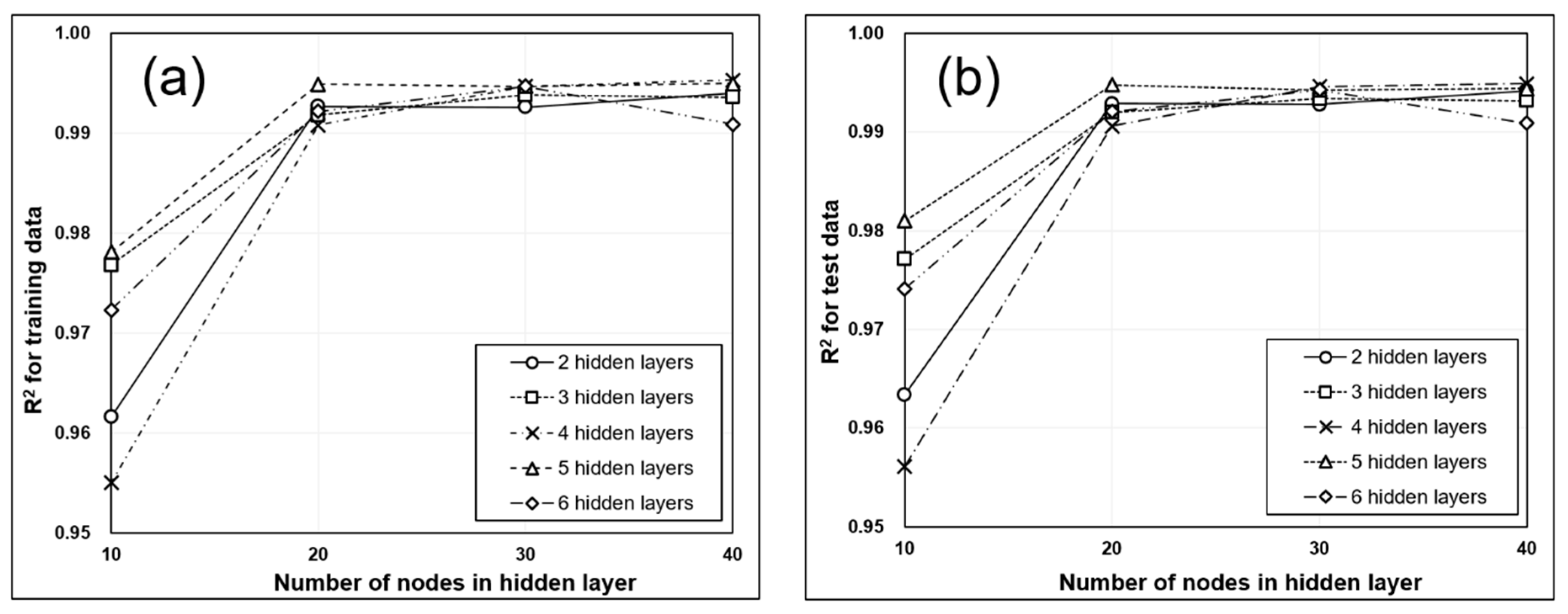
The aim of this study is to present a new method that uses a DNN model to predict the ore production and crusher utilization of an underground mine truck haulage system. An underground limestone mine equipped with an information & communications technology (ICT)-based mine safety management system was selected as the study area. Big data collected for 1 month in October 2018 were processed to create the DNN model training data. The numbers of hidden layers and hidden layer nodes of the DNN model were set to various values, and the coefficient of determination and mean absolute percentage error (MAPE) of the training and test data were analyzed to select the optimal DNN model. The completely trained DNN model was used to predict the ore production and crusher utilization for 10 days, starting on 1 November 2018, and the results were compared with the values observed on site.

2. Study Area

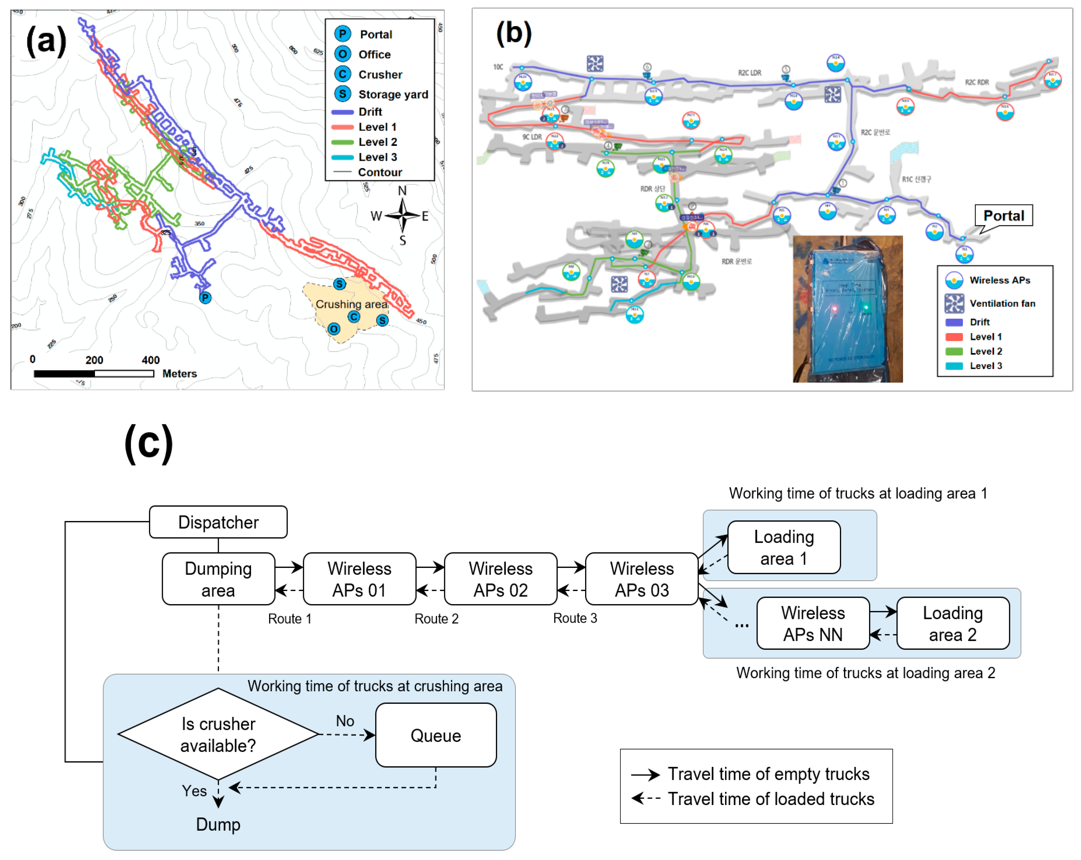
The Baekkwang Mineral Products Yeongcheon underground mine (37°4′14″, 128°18′48″), located in Danyang-gun, Chungcheongbuk-do, South Korea, was selected as the study area. This mine produces 1.2 million tons of limestone annually. The produced limestone is sorted according to its quality and shipped for use in steel, chemicals, and construction materials. The mine interior consists of drifts and three levels, while the exterior includes offices, a crusher, and two storage yards (see Figure 1a).

The study area is equipped with an ICT-based mine safety management system. In such a system, a wireless network environment is created within the underground mine to track the movement of the equipment and workers in real time and to monitor the work environment to prevent casualties. In the study area, 37 wireless access points (APs) were installed in the pit and 3 were installed in the exterior crushing area to create a wireless communication network (see Figure 1b). Wireless APs recognize the tags attached to the equipment and workers, and monitor the work environment in the pit, transmitting the collected information to a server in real time. The web server accumulates real-time data, including whether the equipment and workers have entered the pit, the work times, and data regarding the pit environment (for example, the temperature, humidity, and hazardous gas concentrations). Therefore, the mine safety management system creates big data, which records the mining work on a web server. Further details on the study area mine safety management system and big data can be found in Baek and Choi [23].

In the mine, 25-ton dump trucks travel back and forth between the interior and exterior, hauling ore and waste (see Figure 1c). The production manager considers the average quality of the ore that will be delivered that day, determines the positions and number of production work areas, and notifies the truck drivers of their destinations. The trucks that are provided with their destinations enter through the underground mine entrance and travel to the loading areas via Wireless APs 01, 02, and 03. After a loader has loaded a truck with ore, the truck exits the mine again, travels to the crushing area, and determines whether or not it can unload the ore in a hopper. If there are no trucks waiting to unload, the ore is immediately unloaded in the hopper. If there are trucks waiting, each truck waits for a fixed time. Trucks that have completed unloading enter the mine again to perform further haulage work.

3. Methods

3.1. Principle of DNN

A normal DNN structure consists of an input layer, one or more hidden layers, and an output layer, as illustrated in Figure 2a. Each layer consists of nodes, which are connected to the nodes of the next layer by means of connection links. Figure 2b presents the process of moving through the input layer and hidden layers to produce the target values at the output layer. Equations (1) and (2) present the formula that uses the input variables to calculate the target value, where $x_1$ and $x_2$ are the input variables, $n_1$ and $n_2$ are the hidden layer node values, $f$ is the activation function, $\widehat{y}$ is the target value, $w$ is the weight, and $b$ is the bias. The activation function uses the weighted sum of nodes as the input and converts it into a valid value. The Rectified Linear Unit (ReLU) is a typical nonlinear activation function used in regression analysis [57]. The ReLU outputs zero if the input value (z) is less than 0, and it outputs the same value as the input value if it is greater than 0 (see Equation (3)).

$$n_1=f\left(x_1{w}_{11}+x_2{w}_{21}+b_1\right),n_2=f\left(x_1{w}_{12}+x_2{w}_{22}+b_2\right)$$

(1)

$$\widehat{y}=f\left(n_1{w}_{31}+n_2{w}_{32}+b_3\right)$$

(2)

$$f=\{\begin{array}{cc}z<0& f\left(z\right)=0\\ z\ge 0& f\left(z\right)=z\end{array}$$

(3)

To minimize the error between the predicted and observed values, the weights assigned to the nodes of all layers are modified by a back-propagation method [58] every time the model is trained. This method measures the error function slope using the gradient descent method and updates the weights of all neurons to minimize the error. Typical gradient descent methods include stochastic gradient descent [59], RMSprop [60], and Adam [61]. Equation (4) presents the formula that updates the weights. The weights are adjusted until the partial derivative of the error function is 0. In the equation below, i is the node number of the previous layer, j is the node number of the next layer, $w_{ij}^t$ is the weight at time t, $w_{ij}^{t+1}$ is the updated weight at time t + 1, $\eta$ is the learning rate, and $E$ is the error function.

$$w_{ij}^{t+1}=w_{ij}^t-\eta \frac{\partial E}{\partial w_{ij}}$$

(4)

3.2. Design of DNN Model

Two DNN models were designed to predict the ore production and crusher utilization, as illustrated in Figure 3. The input layer node configurations of the two DNN models are the same. The input layer consists of 26 nodes, among which 8 nodes represent the truck haulage system operating conditions and 18 nodes represent the truck cycle times.

Table 1. Description of input nodes in DNN model.

Type	Node	Description	Unit
Truck haulage operation conditions	${\mathrm{X}}_1$	Total truck haulage operation time	Day
	${\mathrm{X}}_2$	Daily working time	Minutes
	${\mathrm{X}}_3$	Number of dispatched trucks	Minutes
	${\mathrm{X}}_4$	Initial truck dispatch time	Minutes
	${\mathrm{X}}_5$	Truck dispatch interval	Number
	${\mathrm{X}}_6$	Truck loading capacity	Tons
	${\mathrm{X}}_7$	Probability of occurring loading 1	Ratio
	${\mathrm{X}}_8$	Probability of occurring loading 2	Ratio
Truck cycle time	${\mathrm{X}}_9$	Average travel time of empty trucks at route 1	Minutes
	${\mathrm{X}}_{10}$	Standard deviation of travel time of empty trucks at route 1	Minutes
	${\mathrm{X}}_{11}$	Average travel time of empty trucks at route 2	Minutes
	${\mathrm{X}}_{12}$	Standard deviation of travel time of empty trucks at route 2	Minutes
	${\mathrm{X}}_{13}$	Average travel time of empty trucks at route 3	Minutes
	${\mathrm{X}}_{14}$	Standard deviation of travel time of empty trucks at route 3	Minutes
	${\mathrm{X}}_{15}$	Average working time of trucks at loading area 1	Minutes
	${\mathrm{X}}_{16}$	Standard deviation of working time of trucks at loading area 1	Minutes
	${\mathrm{X}}_{17}$	Average working time of trucks at loading area 2	Minutes
	${\mathrm{X}}_{18}$	Standard deviation of working time of trucks at loading area 2	Minutes
	${\mathrm{X}}_{19}$	Average travel time of loaded trucks at route 3	Minutes
	${\mathrm{X}}_{20}$	Standard deviation of travel time of loaded trucks at route 3	Minutes
	${\mathrm{X}}_{21}$	Average travel time of loaded trucks at route 2	Minutes
	${\mathrm{X}}_{22}$	Standard deviation of travel time of loaded trucks at route 2	Minutes
	${\mathrm{X}}_{23}$	Average travel time of loaded trucks at route 1	Minutes
	${\mathrm{X}}_{24}$	Standard deviation of travel time of loaded trucks at route 1	Minutes
	${\mathrm{X}}_{25}$	Average working time of trucks at crushing area	Minutes
	${\mathrm{X}}_{26}$	Standard deviation of Working times of trucks at crushing area	Minutes

displays the types and units of the input nodes. The operating conditions of the truck haulage system include the total truck haulage operation time, daily work time, initial truck dispatch time, truck dispatch interval, number of dispatched trucks, truck loading capacity, probability of Loading 1 occurring, and probability of Loading 2 occurring. Loading 1 occurs when the truck travels to a loading area 1 located near Wireless APs 03 and is loaded with ore. Loading 2 occurs when the truck passes Wireless APs 03 and travels to loading area 2 located farther away than loading area 1. The truck cycle time consists of the empty truck travel time, working time of the trucks at the loading area, loaded truck travel time, and working time of trucks at crushing area. The working time of trucks at the loading area consists of the time required to travel from Wireless APs 03 to the loading area, the time required to load the ore into the trucks, and the time required to return to Wireless APs 03. The output layers of the two DNN models are composed of single nodes, which represent the ore production and crusher utilization, respectively. To configure a hidden layer that can maximize the DNN prediction accuracy, the numbers of hidden layers and hidden layer nodes were set to different values and the models were trained.

3.3. Dataset Preparation for DNN Model

The big data collected by the mining safety management system installed in the study area were processed to create training data for the DNN model. The training data were created according to the following process. The big data (containing information such as the times at which the wireless APs recognized the truck tags during haulage work, the recognized truck tag IDs, and the distances between the wireless APs and tags) were collected on the web server. The big data were processed, and the information required for creating the training data (daily work time, number of dispatched trucks, production, and crusher utilization) was analyzed. The truck travel times for each interval were determined by calculating the time differences in the times at which the wireless APs recognized the truck tags. Finally, the processed data were saved in a suitable format for the training data.

The data that were collected in the study area for 1 month in October 2018 were processed and 9072 training data points were created.

Table 2. Example of training data of DNN model for predicting ore production.

1 420 3 0 6 20 0.8 0.2 3.23 0.83 0.44 0.05 0.37 0.06 5.97 0.81 19.84 3.39 0.46 0.06 0.54 0.06 5.4 0.5 0.11 1280
1 540 5 0 5 25 0.6 0.4 3.23 0.83 0.44 0.05 0.37 0.06 5.97 0.81 19.84 3.39 0.46 0.06 0.54 0.06 5.4 0.5 0.11 2925
1 360 6 0 1 25 1 0 3.23 0.83 0.44 0.05 0.37 0.06 5.97 0.81 19.84 3.39 0.46 0.06 0.54 0.06 5.4 0.5 0.11 2700
1 480 3 0 4 25 0 1 3.23 0.83 0.44 0.05 0.37 0.06 5.97 0.81 19.84 3.39 0.46 0.06 0.54 0.06 5.4 0.5 0.11 2000
1 420 2 0 4 30 0.8 0.2 3.23 0.83 0.44 0.05 0.37 0.06 5.97 0.81 19.84 3.39 0.46 0.06 0.54 0.06 5.4 0.5 0.11 1320
1 720 5 0 4 30 0.6 0.4 3.23 0.83 0.44 0.05 0.37 0.06 5.97 0.81 19.84 3.39 0.46 0.06 0.54 0.06 5.4 0.5 0.11 4860
1 240 6 0 2 20 0.8 0.2 3.23 0.83 0.44 0.05 0.37 0.06 5.97 0.81 19.84 3.39 0.46 0.06 0.54 0.06 5.4 0.5 0.11 1460
1 840 6 0 6 30 1 0 3.23 0.83 0.44 0.05 0.37 0.06 5.97 0.81 19.84 3.39 0.46 0.06 0.54 0.06 5.4 0.5 0.11 8970
$⋮$

presents part of the training data created for the production prediction. For example, in the first row of Table 2, it can be seen that the 3 trucks were dispatched to the haulage operation for 420 min in a day, the initial truck dispatch time was 0 min, and the truck dispatch interval was set to 6 min. Moreover, the truck loading capacity was set to 20 tons, the probability of loading 1 and loading 2 occurring was 0.8:0.2, and ore production was 1280 tons. The truck cycle time was calculated by considering the operational records of all trucks that performed haulage work in October, and it was set to the same value for all training data. It can be observed that the ore production varied according to the changes in the truck haulage work conditions, such as the daily work time, number of dispatched trucks, and truck dispatch interval.

To analyze the correlation between input variables and target values, the Pearson correlation coefficient (PCC) is calculated using training data. Equation (5) presents the formula for calculating the PCC ($r$), where n is the number of samples, $x_i$ and $y_i$ are ith samples, $\overline{x}$ is the mean of $x$ samples, and $\overline{y}$ is the mean of $\mathrm{y}$ samples.

Table 3. Results of correlation analysis between input variables, ore production, and crusher utilization.

Ore Production		Crusher Utilization
Input Variables	$\mathbf{PCC}{}^1\left(\mathit{r}\right)$	Input Variables	$\mathbf{PCC}{}^1\left(\mathit{r}\right)$
Daily working time	0.65	Number of dispatched trucks	0.88
Number of dispatched trucks	0.57	Probability of loading 1 occurring	0.39
Probability of loading 1 occurring	0.24	Daily working time	0.10
Truck loading capacity	0.19	Truck dispatch interval	−0.01
Probability of loading 2 occurring	−0.24	Probability of loading 2 occurring	−0.40

¹ Pearson correlation coefficient.

presents the results of calculating the PCC between input variables, ore production, and crusher utilization. Ore production has a high positive correlation with the daily working time and the number of dispatched trucks, and a low negative correlation with the probability of loading 2 occurring. Crusher utilization has a high positive correlation with the number of dispatched trucks and the probability of loading 1 occurring and a high negative correlation with the probability of loading 2 occurring. Figure 4 illustrates the distributions of the ore production and crusher utilization in the training data. The average ore production was 1708 tons, while the average crusher utilization was 8.74%. Moreover, 75% of the training data was used as the DNN model learning data, and 25% was used as the test data.

$$r=\frac{{{\displaystyle \sum }}_{i=1}^n\left(x_i-\overline{x}\right)\left(y_i-\overline{y}\right)}{\sqrt{{{\displaystyle \sum }}_{i=1}^n{\left(x_i-\overline{x}\right)}^2}\sqrt{{{\displaystyle \sum }}_{i=1}^n{\left(y_i-\overline{y}\right)}^2}}$$

(5)

3.4. Experimental Setup for DNN Model Training

To determine the optimal hidden layer structure for the DNN model, the number of hidden layers and hidden layer nodes were set to various values while the models were trained, and the prediction accuracy of the models was evaluated.

Table 4. Description of hidden layer setting of DNN model.

Configuration of the Hidden Layer						No. of Cases
No. of Hidden Layer			No. of Nodes in Hidden Layer
From	To	Interval	From	To	Interval
2	6	1	10	40	10	20

presents the numbers of hidden layers and hidden layer nodes used to train the DNN model. The total number of hidden layers in the DNN model was set to between two and six, while the number of hidden layer nodes was set to between 10 and 40.

The prediction accuracy of the DNN model was evaluated by means of the coefficient of determination and MAPE. Equations (6)–(8) present the formulae for calculating the coefficient of determination between the observed and predicted values, where ${\mathrm{R}}^2$ is the coefficient of determination, SSR is the sum of the squared residual, SSD is the sum of the squared variance, N is the number of training data points, $y_i$ is the observed value of the i-th training data point, ${\widehat{y}}_i$ is the predicted value of the i-th training data point, and $\overline{y}$ is the average of the observed values. Equation (9) presents the formula for calculating the MAPE.

$${\mathrm{R}}^2=1-\frac{\mathrm{SSR}}{\mathrm{SSD}}$$

(6)

$$\mathrm{SSR}={\displaystyle \sum }_{i=1}^N{\left(y_i-{\widehat{y}}_i\right)}^2$$

(7)

$$\mathrm{SSD}={\displaystyle \sum }_{i=1}^n{\left(y_i-\overline{y}\right)}^2$$

(8)

$$\mathrm{MAPE}=\frac{1}{\mathrm{N}}{\displaystyle \sum }_{i=1}^{\mathrm{N}}\frac{\left|y_i-{\widehat{y}}_i\right|}{y_i}\times 100(\%)$$

(9)

An algorithm was developed using the Python language to train the DNN models. Figure 5 illustrates the algorithm execution process of the DNN model training. Firstly, the Python modules required to train the DNN model (such as Keras [62], TensorFlow [63], and NumPy [64]) and the training data are entered as inputs, and the training data are divided at a fixed ratio to create the test data. Next, the structure of the DNN model input, hidden, and output layers is configured, and the activation function for each layer is defined. When the actual DNN model training begins, the epoch (number of training rounds) is incremented by 1. The trained DNN model is used to predict the test data and the prediction error is calculated. If the epoch is 1, the minimum error is defined as the prediction error, and the patience is defined as 0. In this case, the patience is the number of times that the prediction error is not reduced. If the patience exceeds a fixed number, the training is terminated early to prevent model over-fitting. If the number of training times is 2 or more and the prediction error is less than the minimum error, the minimum error is updated as the prediction error and the patience is updated as 0. At this point, the DNN model is saved as the optimal model. When the training is terminated once, the hidden and output layer weights are modified, and the model is trained again. If the number of training times reaches the maximum epoch limit (MAX_epoch) or the patience reaches the maximum patience limit (MAX_patience), the model training is terminated. In this study, the algorithm setting MAX_epoch was set to 1000, while MAX_patience was set to 200 for the DNN model training. All of the activation functions in the input layer and hidden layers were set to ReLU, and the Adam optimizer was used to update the weights.

3.5. Inference Using DNN Model

After comparing the prediction accuracy of the trained DNN models, that with the highest coefficient of determination and lowest MAPE for the test data was selected as the optimal model. To verify the optimal DNN model, the model was used to predict the ore production and crusher utilization occurring during truck haulage work over the course of 10 days, starting on 1 November 2018. Moreover, the values predicted by the DNN model were compared to those observed at the actual mining site. The ore production at the actual mining site was calculated based on the number of times that the trucks hauled ore and the truck loading capacity. The crusher utilization was calculated by Equation (10), where UR is the crusher utilization (%), NH is the number of times that ore is hauled, AWT is the average working time of trucks at crushing area (min), and DWT is the daily work time (min). AWT was set to 0.59 min for all work days.

$$\mathrm{UR}=\frac{\mathrm{NH}\times \mathrm{AWT}\times 100}{\mathrm{DWT}}(\%)$$

(10)

The DNN model input nodes were set to be the same as the operating schedule for the truck haulage work performed over the 10 days.

Table 5. Description of input node setting of optimal DNN model for predicting ore production and crusher utilization over 10 working days.

Input Parameters	Date
	11/1	11/2	11/5	11/6	11/7	11/8	11/9	11/15	11/16	11/17
Daily working time (min)	630	360	791	557	426	910	446	461	404	431
Probability of occurring loading 1	0	0	0.3	0	0	0	0	0	0	0.33
Probability of occurring loading 2	1	1	0.7	1	1	1	1	1	1	0.67

displays the DNN model input node values that were set to predict the ore production and crusher utilization. The number of trucks dispatched on all days was set to 1, the truck dispatch interval was set to 1 min, the truck loading capacity was set to 30 tons, the total truck haulage work days was set to 1, and the first truck dispatch time was set to 0 min.

The root mean square error (RMSE) between the observed and calculated values was calculated to determine the error for the ore production and crusher utilization predicted by the optimized DNN model (see Equation (11)).

$$\mathrm{RMSE}=\sqrt{\frac{{{\displaystyle \sum }}_{i=1}^n{\left(y_i-{\widehat{y}}_i\right)}^2}{n}}$$

(11)

4. Results

4.1. Experimental Evaluation of Trained DNN Models

The prediction accuracy of the DNN model training and test data was analyzed. Figure 6 illustrates the coefficient of determination and MAPE for the training and test data, according to the numbers of hidden layers and hidden layer nodes of the DNN model. As the number of hidden layer nodes increased, the coefficient of determination for the training and test data gradually increased, without regard to the number of hidden layers, while the MAPE gradually decreased.

When the number of hidden layer nodes was set to 20 or more, the coefficient of determination for all of the DNN model training and test data was found to be 0.99, while the MAPE was less than 5%.

When the number of hidden layers of the DNN model was set to five and the number of hidden layer nodes was set to 40; the coefficient of determination for the test data was the highest at approximately 0.99; and the MAPE was the lowest at approximately 2.80% (see

Table 6. Evaluation results of coefficient of determination and MAPE of DNN model with five hidden layers and 40 hidden layer nodes for ore production prediction.

Data Type	Statistics
	$\mathbf{Coefficient}\mathbf{of}\mathbf{Determination}\left({\mathbf{R}}^2\right)$	MAPE (%)
Training data	0.99	2.45
Test data	0.99	2.80

). Moreover, the coefficient of determination for the training data in this case was approximately 0.99, while the MAPE was approximately 2.45%. Therefore, the DNN model trained with five hidden layers and 40 hidden layer nodes was selected as the optimal model for the ore production prediction.

Figure 7 illustrates the results of using the optimal DNN model for predicting the ore production by predicting the training data and test data, and then analyzing the correlation between the observed and predicted values. The coefficient of determination for the training and test data was found to be greater than 0.99, and the optimal DNN model could accurately predict both the training and test data.

The coefficient of determination and MAPE for the training and test data of the DNN model trained to predict the crusher utilization were analyzed. Figure 8 illustrates the changes in the DNN model coefficient of determination and MAPE for the training and test data with various configurations of the hidden layer structure. As the number of hidden layer nodes increased, the prediction accuracy for the training and test data increased, and the error decreased, without regard to the number of hidden layers. However, when the number of hidden layers was set to 6, the coefficient of determination decreased, and the MAPE increased further when the number of hidden layer nodes increased to a maximum of 40 compared to when the number of hidden layer nodes was set to 30.

Among the 20 hidden layer structure conditions, that with the highest coefficient of determination and lowest MAPE for the test data was the structure with four hidden layers and 40 hidden layer nodes. Therefore, the DNN model trained under these conditions was selected as the optimal DNN model for predicting the crusher utilization.

Table 7. Results of evaluating coefficient of determination and MAPE of optimal DNN model, with four hidden layers and 40 hidden layer nodes, for predicting crusher utilization.

Data Type	Statistics
	$\mathbf{Coefficient}\mathbf{of}\mathbf{Determination}\left({\mathbf{R}}^2\right)$	MAPE (%)
Training data	0.99	2.30
Test data	0.99	2.49

displays the coefficient of determination and MAPE values for the training and test data of the optimal DNN model. The coefficient of determination for the training data was approximately 0.99, while the MAPE was approximately 2.30%. The coefficient of determination for the test data was approximately 0.99, while the MAPE was approximately 2.49%.

Figure 9 illustrates the results of using the optimal DNN model to predict the training and test data for the crusher utilization and analyzing the correlation between the predicted and observed values. In both cases, a high correlation was observed between the predicted and observed values.

4.2. Results of Inference with Optimal DNN Model

The optimal DNN model was used to predict the ore production and crusher utilization over 10 days, starting on 1 November 2018. Figure 10 presents a comparison of the ore production observed at the actual mining site and that predicted by the optimal DNN model. The ore production predicted by the DNN model matched the actual observed values for most days. However, in the case of 7 November, the observed values did not match those predicted by the DNN model. This is because the trucks repeatedly visited a path with a longer travel distance than the path normally visited throughout the overall haulage task. Therefore, the actual observed ore production was lower than the value predicted by the DNN model.

Table 8. RMSE of optimal DNN model for predicted ore production during 10 working days (case 1) and predicted values excluding 7 November (case 2).

Statistics	Case 1	Case 2
RMSE (tons)	10.16	6.92

displays the RMSE of 10 days of ore production, as predicted by the optimal DNN (case 1), and the RMSE of 9 days of ore production, excluding 7 November (case 2). The RMSE of the 10 days of ore production as predicted by the DNN model was approximately 10 tons. The RMSE of the 9 days of ore production was approximately 7 tons.

Figure 11 presents a graph comparing the crusher utilization observed over 10 days while the haulage work was performed at the mine site and the values predicted by the optimal DNN model. The values observed over the 10 days tended to match the crusher utilization predicted by the DNN model. However, as with the ore production, the crusher utilization observed on 7 November differed from the predicted value.

Table 9. RMSE of DNN model for predicted crusher utilization over 10 working days (case 1) and predicted value excluding 7 November (case 2).

Statistics	Case 1	Case 2
RMSE (%)	0.07	0.04

displays the RMSE of 10 days of crusher utilization as predicted by the DNN model (case 1) and the RMSE of 9 days of crusher utilization, excluding 7 November (case 2). The RMSE of the 10 days of crusher utilization was approximately 0.07%, while that of the 9 days of crusher utilization was comparatively low at approximately 0.04%.

5. Discussion

5.1. Correlation of Ore Production and Crusher Utilization

The PCC between ore production and crusher utilization was calculated using training data for the correlation analysis. The PCC between two target values was approximately 0.7, and it was confirmed that the two target values have a high positive correlation. Figure 12 illustrates the results of correlation analysis between two target values. Training data in zone A have a high positive correlation, and the data in zone B show a low positive correlation. The criteria for classifying zone A and zone B in the graph are daily working time and number of dispatched trucks based on the training data. It was found that the daily working time and number of dispatched trucks of training data in zone A, which individually have a significant impact on ore production and crusher utilization, were both simultaneously high. In contrast, in zone B, the number of dispatched trucks of training data was high, but the daily working time was low.

5.2. Application of DNN Models for Haulage Operation Planning

To design and plan the truck haulage work at a mining site, a production manager must first predict and analyze the short-term and long-term ore production and crusher utilization. The DNN model designed in this study can be used to predict the ore production and crusher utilization, as it changes according to the daily work time, number of trucks, and truck dispatch interval, among others, and can efficiently design haulage tasks.

In this study, an optimal DNN model was used to analyze the changes in ore production and crusher utilization according to the number of trucks and truck dispatch interval, while considering the operational conditions of the ore haulage work performed by the trucks on 5 November 2018. A daily working time of 13 h and 11 min (791 min), a truck load capacity of 30 tons, and a daily ore production target of 3000 tons were assumed. Moreover, it was assumed that the number of times the truck visits the loading area had already been determined according to the quality of the delivered ore. The probability of Loading 1 occurring was set to 0.27, while the probability of Loading 2 occurring was set to 0.73.

Figure 13a presents the results of using the optimal DNN model to analyze the ore production and crusher utilization, according to the number of trucks. As the number of trucks contributing to the ore haulage work increased, the ore production and crusher utilization exhibited an increasing trend. To satisfy the daily ore production targets, four or more trucks must be used in the haulage work, and the crusher utilization in this case is 9% or higher. Figure 13b illustrates the results of using the optimal DNN model to analyze the changes in the ore production and crusher utilization according to the truck dispatch interval, assuming that four trucks contributed to the haulage work. Even when the truck dispatch interval increased, the ore production was maintained at approximately 3500 tons and the crusher utilization was maintained at approximately 9%. To maximize the ore production, it is helpful to set the truck dispatch interval to approximately 1 to 2 min.

6. Conclusions

In this study, a DNN-based deep learning model was trained for predicting the ore production and crusher utilization of a truck haulage system in an underground mine. An underground limestone mine was selected as the study area, and the DNN model input nodes were configured to reflect the truck haulage system of the study area. The DNN model was trained by setting various hidden layer configurations, and the coefficient of determination and MAPE for the training and test data were calculated to evaluate the model prediction accuracy. The DNN model was trained considering the haulage work operating conditions in the study area, and it was used to predict the ore production and crusher utilization over 10 days, starting on 1 November 2018. The predicted results were compared with the actual observed results.

The prediction accuracy for the ore production was the highest when the number of hidden layers of the DNN model was set to four and the number of hidden layer nodes was set to 40. In this case, the coefficient of determination for the test data was approximately 0.99, while the MAPE was approximately 2.80%. The prediction accuracy for the crusher utilization was the highest when the number of hidden layers of the DNN model was set to four and the number of hidden layer nodes was set to 40. In this case, the coefficient of determination for the test data was approximately 0.99, while the MAPE was approximately 2.49%. The predicted ore production and crusher utilization for the 9 days of haulage work excluding 7 November tended to match the observed values. On 7 November, the trucks used a haulage path longer than that normally used to haul ore, and as a result, the predicted and observed values did not match. The RMSE of the ore prediction for the 9 days excluding 7 November was approximately 6.92 tons, while that for the crusher utilization was approximately 0.04%.

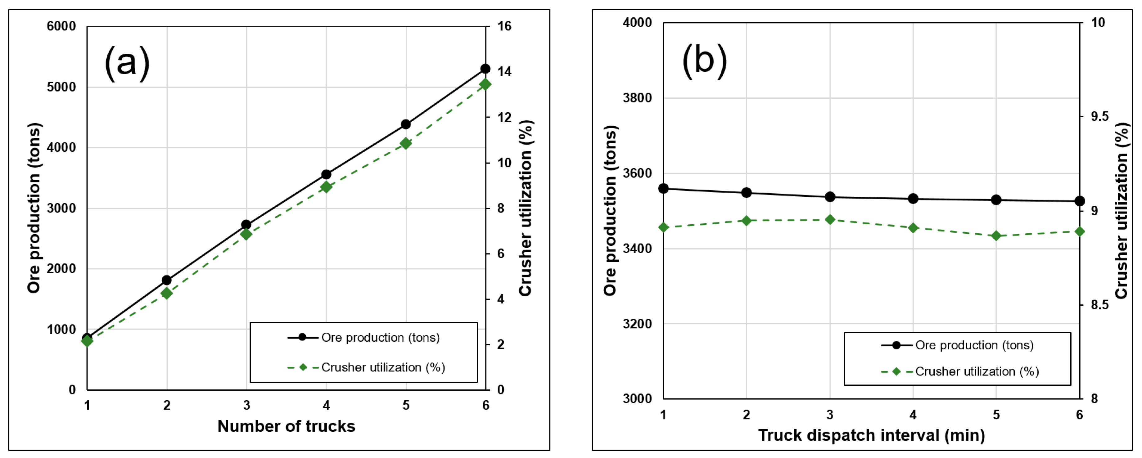
The DNN model input nodes were set considering the operating conditions of the ore haulage work performed on 5 November 2018. The number of trucks and truck dispatch interval were set to various values, and the changes in the ore production and crusher utilization were predicted. The results demonstrated that a daily ore production target of 3000 tons can be satisfied if the number of ore haulage trucks is set to four and the truck dispatch interval is set to 1 to 2 min. It was confirmed that the DNN model-based ore production and crusher utilization prediction methods presented in this study can be used for short-term or long-term mine haulage system design and prediction.

We trained the DNN models for ore production and crusher utilization prediction and tested them on the first 10 days of the following month. The DNN models predicted the target values accurately for 9 days; however, the models could not accurately predict the target value on the day the truck took a different path than usual. This may mean that the DNN models were successful because there was not a lot of variation between the routines of each day. The DNN models may only be memorizing the outputs given the inputs (over-fitting), which would make them very unreliable. To solve this problem, the models must be further trained such that the varying conditions of the mine can be taken into account. Alternatively, by training the model on a longer time span, all possible paths can be used as input parameters, and over-fitting can be avoided. Therefore, further studies are required in order to select a reasonable DNN model update cycle and determine the training data acquisition time span to consider various types of changing conditions in mines.

The results of the study confirmed that a DNN-based deep learning technique can learn sequential operations of a truck haulage system and analyze the correlation between truck haulage system operating conditions, ore production, and crusher utilization using big data acquired from the study area without human inference and algorithms based on prior knowledge. Moreover, it was found that trained DNN models can predict ore production and crusher utilization for 9 working days with low prediction errors. Thus, it would be possible to complement the limitations of existing algorithm-based simulation techniques.

In this study, a DNN model was selected from a variety of deep learning models and used to predict the ore production and crusher utilization. If time series data on ore production are collected to train an RNN model, the change patterns in the ore production over time can be analyzed, and the flow of future ore production changes can be predicted. Furthermore, if the costs of the ore production and haulage are considered and the mining rate of return is predicted, long-term operational mining plans can be established. Therefore, in the future, it will be necessary to perform additional studies on the use of various deep-learning models other than a DNN model to design and predict haulage systems.

References

1. Awuah-Offei, K. Energy efficiency in mining: A review with emphasis on the role of operators in loading and hauling operations. J. Clean. Prod. 2016, 117, 89–97. [Google Scholar] [CrossRef]
2. Subtil, R.F.; Silva, D.M.; Alves, J.C. A Practical Approach to Truck Dispatch for Open Pit Mines. In Proceedings of the 35th APCOM symposium, Wollongong, NSW, Australia, 24–30 September 2011; Baafi, E.Y., Kininmonth, R.J., Porter, I., Eds.; AusIMM: Carlton South, Victoria, Australia, 2011; pp. 765–777. [Google Scholar]
3. Salama, A.; Greberg, J. Optimization of Truck-Loader haulage system in an underground mine: A simulation approach using SimMine. In Proceedings of the MassMin 2012: 6th International Conference & Exhibition on Mass Mining, Sudbury, ON, Canada, 10–14 June 2012; Canadian Institute of Mining, Metallurgy and Petroleum: Sudbury, ON, Canada, 2012; pp. 1–10. [Google Scholar]
4. Mena, R.; Zio, E.; Kristjanpoller, F.; Arata, A. Availability-based simulation and optimization modeling framework for open-pit mine truck allocation under dynamic constraints. Int. J. Min. Sci. Technol. 2013, 23, 113–119. [Google Scholar] [CrossRef]
5. Salama, A.; Nehring, M.; Greberg, J. Operating value optimisation using simulation and mixed integer programming. Int. J. Min. Reclam. Environ. 2014, 28, 25–46. [Google Scholar] [CrossRef]
6. Tarshizi, E.; Sturgul, J.; Ibarra, V.; Taylor, D. Simulation and animation model to boost mining efficiency and enviro-friendly in multi-pit operations. Int. J. Min. Sci. Technol. 2015, 25, 671–674. [Google Scholar] [CrossRef]
7. Soofastaei, A.; Aminossadati, S.M.; Kizil, M.S.; Knights, P. A discrete-event model to simulate the effect of truck bunching due to payload variance on cycle time, hauled mine materials and fuel consumption. Int. J. Min. Sci. Technol. 2016, 26, 745–752. [Google Scholar] [CrossRef]
8. Afrapoli, A.M.; Askari-Nasab, H. Mining fleet management systems: A review of models and algorithms. Int. J. Min. Reclam. Environ. 2019, 33, 42–60. [Google Scholar] [CrossRef]
9. Park, S.; Choi, Y.; Park, H. Optimization of Truck-loader Haulage Systems in an Underground Mine Using Simulation Methods. Geosyst. Eng. 2016, 19, 222–231. [Google Scholar] [CrossRef]
10. Upadhyay, S.P.; Askari-nasab, H. Simulation and optimization approach for uncertainty-based short-term planning in open pit mines. Int. J. Min. Sci. Technol. 2018, 28, 153–166. [Google Scholar] [CrossRef]
11. Samanta, B.; Sarkar, B.; Mukherjee, S.K. Selection of opencast mining equipment by a multi-criteria decision-making process. Min. Technol. 2002, 111, 136–142. [Google Scholar] [CrossRef]
12. Ercelebi, S.G.; Bascetin, A. Optimization of shovel-truck system for surface mining. J. S. Afr. Inst. Min. Metall. 2009, 109, 433–439. [Google Scholar]
13. Salama, A.; Greberg, J.; Schunnesson, H. The use of discrete event simulation for underground haulage mining equipment selection. Int. J. Min. Miner. Eng. 2014, 5, 256–271. [Google Scholar] [CrossRef]
14. Dindarloo, S.R.; Osanloo, M.; Frimpong, S. A stochastic simulation framework for truck and shovel selection and sizing in open pit mines. J. S. Afr. Inst. Min. Metall. 2015, 115, 209–219. [Google Scholar] [CrossRef]
15. Ta, C.H.; Ingolfsson, A.; Doucette, J. A linear model for surface mining haul truck allocation incorporating shovel idle probabilities. Eur. J. Oper. Res. 2013, 231, 770–778. [Google Scholar] [CrossRef]
16. Chaowasakoo, P.; Seppälä, H.; Koivo, H.; Zhou, Q. Digitalization of mine operations: Scenarios to benefit in real-time truck dispatching. Int. J. Min. Sci. Technol. 2017, 27, 229–236. [Google Scholar] [CrossRef]
17. Fadin, A.Y.F.; Moeis, A.O. Simulation-optimization truck dispatch problem using look-ahead algorithm in open pit mines. Int. J. GEOMATE 2017, 13, 80–86. [Google Scholar] [CrossRef]
18. Sembakutti, D.; Kumral, M.; Sasmito, A.P. Analysing equipment allocation through queuing theory and Monte-Carlo simulations in surface mining operations. Int. J. Min. Miner. Eng. 2017, 8, 56–69. [Google Scholar] [CrossRef]
19. Temeng, V.A.; Otuonye, F.O.; Frendewey, J.O. A nonpreemptive goal programming approach to truck dispatching in open pit mines. Miner. Resour. Eng. 1998, 7, 59–67. [Google Scholar] [CrossRef]
20. Gamache, M.; Grimard, R.; Cohen, P. A Shortest-path Algorithm for Solving the Fleet Management Problem in Underground Mines. Eur. J. Oper. Res. 2005, 166, 497–506. [Google Scholar] [CrossRef]
21. Beaulieu, M.; Gamache, M. An Enumeration Algorithm for Solving the Fleet Management Problem in Underground Mines. Comput. Oper. Res. 2006, 33, 1606–1624. [Google Scholar] [CrossRef]
22. Choi, Y.; Park, H.D.; Sunwoo, C.; Clarke, K.C. Multi-criteria evaluation and least-cost path analysis for optimal haulage routing of dump trucks in large scale open-pit mines. Int. J. Geogr. Inf. Sci. 2009, 23, 1541–1567. [Google Scholar] [CrossRef]
23. Baek, J.; Choi, Y. Simulation of Truck Haulage Operations in an Underground Mine Using Big Data from an ICT-Based Mine Safety Management System. Appl. Sci. 2019, 9, 2639. [Google Scholar] [CrossRef]
24. Najafabadi, M.M.; Villanustre, F.; Khoshgoftaar, T.M.; Seliya, N.; Wald, R.; Muharemagic, E. Deep learning applications and challenges in big data analytics. J. Big Data 2015, 2, 1–21. [Google Scholar] [CrossRef]
25. Zhang, Q.; Yang, L.T.; Chen, Z.; Li, P. A survey on deep learning for big data. Inf. Fusion 2018, 42, 146–157. [Google Scholar] [CrossRef]
26. Sze, V.; Chen, Y.; Yang, T.; Emer, J.S. Efficient Processing of Deep Neural Networks: A Tutorial and Survey. Proc. IEEE 2017, 105, 2295–2329. [Google Scholar] [CrossRef] [Green Version]
27. Schmidhuber, J. Deep learning in neural networks: An overview. Neural Netw. 2015, 61, 85–117. [Google Scholar] [CrossRef] [PubMed] [Green Version]
28. Bourlard, H.; Kamp, Y. Auto-Association by Multilayer Perceptrons and Singular Value Decomposition. Biol. Cybern. 1988, 59, 291–294. [Google Scholar] [CrossRef]
29. Gardner, M.W.; Dorling, S. Artificial neural networks (the multilayer perceptron)-A review of applications in the atmospheric sciences. Atmos. Environ. 1998, 32, 2627–2636. [Google Scholar] [CrossRef]
30. Liu, W.; Wang, Z.; Liu, X.; Zeng, N.; Liu, Y.; Alsaadi, F.E. A survey of deep neural network architectures and their applications. Neurocomputing 2017, 234, 11–26. [Google Scholar] [CrossRef]
31. Goodfellow, I.; Bengio, Y.; Courville, A. Deep Learning (Adaptive Computation and Machine Learning Series); The MIT Press: Cambridge, MA, USA, 2019; pp. 1–800. ISBN 978-0262035613. [Google Scholar]
32. Deng, L. Three Classes of Deep Learning Architectures and Their Applications: A Tutorial Survey. APSIPA Trans. Signal Inf. Process. 2012, 3, 1–28. [Google Scholar]
33. Fukushima, K. Neocognitron: A Self-Organizing Neural Network Model for a Mechanism of Pattern Recognition Unaffected by Shift in Position. Biol. Cybern. 1980, 36, 193–202. [Google Scholar] [CrossRef]
34. Lecun, Y.; Bengio, Y.; Hinton, G. Deep learning. Nature 2015, 521, 436–444. [Google Scholar] [CrossRef] [PubMed]
35. Sutskever, I.; Martens, J.; Hinton, G. Generating Text with Recurrent Neural Networks. In Proceedings of the 28th International Conference on Machine Learning, Bellevue, WA, USA, 28 June–2 July 2011; Getoor, L., Scheffer, T., Eds.; Omnipress: Madison, WI, USA, 2011; pp. 1017–1024. [Google Scholar]
36. Graves, A.; Mohamed, A.; Hinton, G. Speech recognition with deep recurrent neural networks. In Proceedings of the 2013 IEEE International Conference on Acoustics, Speech and Signal Processing, Vancouver, BC, Canada, 26–31 May 2013; IEEE: New York, NY, USA, 2013; pp. 6645–6649. [Google Scholar] [Green Version]
37. Gehring, J.; Miao, Y.; Metze, F. Extracting Deep Bottleneck Features Using Stacked Auto-encoders. In Proceedings of the 2013 IEEE International Conference on Acoustics, Speech and Signal Processing, Vancouver, BC, Canada, 26–31 May 2013; IEEE: New York, NY, USA, 2013; pp. 3377–3381. [Google Scholar]
38. Weng, R.; Lu, J.; Member, S.; Tan, Y.; Member, S. Learning Cascaded Deep Auto-Encoder Networks for Face Alignment. IEEE Trans. Multimed. 2016, 18, 2066–2078. [Google Scholar] [CrossRef]
39. Hinton, G.E.; Osindero, S.; Teh, T.W. A fast learning algorithm for deep belief nets. Neural Comput. 2006, 18, 1527–1554. [Google Scholar] [CrossRef] [PubMed]
40. Hinton, G.E.; Salakhutdinov, R.R. Reducing the Dimensionality of Data with Neural Networks. Science 2006, 313, 504–508. [Google Scholar] [CrossRef] [PubMed]
41. Xiong, Y.; Zuo, R. Recognition of geochemical anomalies using a deep autoencoder network. Comput. Geosci. 2016, 86, 75–82. [Google Scholar] [CrossRef]
42. Li, W.; Wu, G.; Du, Q. Transferred Deep Learning for Anomaly Detection in Hyperspectral Imagery. IEEE Geosci. Remote Sens. Lett. 2017, 14, 597–601. [Google Scholar] [CrossRef]
43. Zhang, S.; Xiao, K.; Carranza, E.J.M.; Yang, F.; Zhao, Z. Computers and Geosciences Integration of auto-encoder network with density-based spatial clustering for geochemical anomaly detection for mineral exploration. Comput. Geosci. 2019, 130, 43–56. [Google Scholar] [CrossRef]
44. Brown, W.M.; Gedeon, T.D.; Groves, D.I.; Barnes, R.G. Artificial neural networks: A new method for mineral prospectivity mapping. Aust. J. Earth Sci. 2000, 47, 757–770. [Google Scholar] [CrossRef]
45. Leite, E.P.; de Souza Filho, C.R. Artificial neural networks applied to mineral potential mapping for copper-gold mineralizations in the Carajás Mineral Province, Brazil. Geophys. Prospect. 2009, 57, 1049–1065. [Google Scholar] [CrossRef]
46. Oh, H.; Lee, S. Application of Artificial Neural Network for Gold-Silver Deposits Potential Mapping: A Case Study of Korea. Nat. Resour. Res. 2010, 19, 103–124. [Google Scholar] [CrossRef]
47. Xiong, Y.; Zuo, R.; John, E.; Carranza, M. Mapping mineral prospectivity through big data analytics and a deep learning algorithm. Ore Geol. Rev. 2018, 102, 811–817. [Google Scholar] [CrossRef]
48. Huang, L.; Balamurali, M.; Silversides, K.L. Machine learning classification of geochemical and geophysical data. In Proceedings of the 39th International Symposium ‘Application of Computers and Operations Research in the MIneral Industry’(APCOM 2019), Wroclaw, Poland, 4–6 June 2019; Mueller, C., Assibey-Bonsu, W., Baafi, E., Dauber, C., Doran, C., Jaszczuk, M.J., Nagovitsyn, O., Eds.; CRC Press: London, UK, 2019; pp. 101–105. [Google Scholar]
49. Sayadi, A.R.; Fathianpour, N.; Mousavi, A. Open pit optimization in 3D using a new artificial neural network. Arch. Min. Sci. 2011, 56, 389–403. [Google Scholar]
50. Huang, L.; Li, J.; Hao, H.; Li, X. Micro-seismic event detection and location in underground mines by using Convolutional Neural Networks (CNN) and deep learning. Tunn. Undergr. Space Technol. 2018, 81, 265–276. [Google Scholar] [CrossRef]
51. Geise, S.; Emery, J.; Canbulat, I. Assessment of development roadway roof conditions at an operating underground coal mine using neural network analysis. In Proceedings of the 2019 Coal Operators Conference, Wollongong, NSW, Australia, 18–20 February 2019; Aziz, N., Kininmonth, B., Eds.; The University of Wollongong Printery: Wollongong, NSW, Australia, 2019; pp. 66–81. [Google Scholar]
52. Hu, F.; Zhou, M.; Yan, P.; Li, D.; Lai, W.; Bian, K.; Dai, R. Identification of mine water inrush using laser-induced fluorescence spectroscopy combined with one-dimensional convolutional neural network. RSC Adv. 2019, 9, 7673–7679. [Google Scholar] [CrossRef] [Green Version]
53. Soofastaei, A.; Aminossadati, S.M.; Kizil, M.S.; Knights, P. Reducing Fuel Consumption of Haul Trucks in Surface Mines Using Artificial Intelligence Models. In Proceedings of the 2016 Coal Operators’ Conference, Wollongong, NSW, Australia, 10–12 February 2016; Aziz, N., Kininmonth, B., Eds.; The University of Wollongong Printery: Wollongong, NSW, Australia, 2019; pp. 477–489. [Google Scholar]
54. Xu, J.; Wang, Z.; Tan, C.; Lu, D.; Wu, B.; Su, Z.; Tang, Y. Cutting Pattern Identification for Coal Mining Shearer through Sound Signals Based on a Convolutional Neural Network. Symmetry 2018, 10, 736. [Google Scholar] [CrossRef]
55. Gorai, A.K.; Balusa, B.C.; Sameer, U. A deep learning approach for automated quality control of iron ores. In Proceedings of the 39th International Symposium ‘Application of Computers and Operations Research in the MIneral Industry’(APCOM 2019), Wroclaw, Poland, 4–6 June 2019; Mueller, C., Assibey-Bonsu, W., Baafi, E., Dauber, C., Doran, C., Jaszczuk, M.J., Nagovitsyn, O., Eds.; CRC Press: London, UK, 2019; pp. 455–462. [Google Scholar]
56. Niquini, F.G.F.; Costa, J.F.C.L. Comparison between regression models and neural networks applied to forecast geometallurgical variables. In Proceedings of the 39th International Symposium ‘Application of Computers and Operations Research in the MIneral Industry’(APCOM 2019), Wroclaw, Poland, 4–6 June 2019; Mueller, C., Assibey-Bonsu, W., Baafi, E., Dauber, C., Doran, C., Jaszczuk, M.J., Nagovitsyn, O., Eds.; CRC Press: London, UK, 2019; pp. 463–472. [Google Scholar]
57. Glorot, X.; Bordes, A.; Bengio, Y. Deep Sparse Rectifier Neural Networks. In Proceedings of the 14th International Conference on Artificial Intelligence and Statistics, Ft. Lauderdale, FL, USA, 11–13 April 2011; Gordon, G., Dunson, D., Dudik, M., Eds.; JMLR W&CP: Brookline, MA, USA, 2011; pp. 315–323. [Google Scholar]
58. Rumelhart, D.E.; Hinton, G.E.; Williams, R.J. Learning Representations by Back-Propagating Errors. In Cognitive Modeling; Polk, T.A., Seifert, C.M., Eds.; The MIT Press: Cambridge, MA, USA, 2002; pp. 213–220. ISBN 0-262-66116-0. [Google Scholar]
59. Bottou, L. Large-Scale Machine Learning with Stochastic Gradient Descent. In Proceedings of the COMPSTAT’2010, Paris, France, 22–27 August 2010; Lechevallier, Y., Saporta, G., Eds.; Springer-Verlag: Berlin/Heidelberg, Germany, 2010; pp. 177–186. [Google Scholar] [Green Version]
60. Hinton, G.; Srivastava, N.; Swersky, K. Neural Networks for Machine Learning. Available online: http://www.cs.toronto.edu/~tijmen/csc321/slides/lecture_slides_lec6.pdf (accessed on 27 August 2019).
61. Kingma, D.P.; Ba, J.L. ADAM: A Method for Stochastic Optimization. In Proceedings of the ICLR 2015, Vancouver Convention Center, Vancouver, BC, Canada, 7–9 May 2015; pp. 1–15. [Google Scholar]
62. Keras Documentation. Available online: https://keras.io/ (accessed on 27 August 2019).
63. Tensorflow. Available online: https://www.tensorflow.org/ (accessed on 27 August 2019).
64. Numpy Documentation. Available online: https://www.numpy.org/ (accessed on 27 August 2019).
Figure 1. Schematics of study area: (a) mine map indicating underground drifts and outside crushing area; (b) location map of wireless APs along haulage road in underground mine; (c) process of haulage operation system.
Applsci 09 04180 g001
Figure 2. Description of DNN model: (a) structure of DNN model; (b) process for forecasting output through DNN model.
Applsci 09 04180 g002
Figure 3. Design of DNN model for predicting ore production and crusher utilization.
Applsci 09 04180 g003
Figure 4. Histogram of training data: (a) ore production; (b) crusher utilization.
Applsci 09 04180 g004
Figure 5. Flowchart illustrating procedures for DNN model training algorithm.
Applsci 09 04180 g005
Figure 6. Results of accuracy analysis of DNN models for predicting ore production with different numbers of hidden layers and hidden layer nodes: coefficient of determination for (a) training data and (b) test data, and MAPE for (c) training data and (d) test data.
Applsci 09 04180 g006aApplsci 09 04180 g006b
Figure 7. Results of correlation analysis between measured and predicted ore production (tons) using optimal DNN model with five hidden layers and 40 hidden layer nodes: (a) training data and (b) test data.
Applsci 09 04180 g007
Figure 8. Results of accuracy analysis of DNN models for predicting crusher utilization with different numbers of hidden layers and hidden layer nodes: coefficient of determination for (a) training data and (b) test data, and MAPE for (c) training data and (d) test data.
Applsci 09 04180 g008aApplsci 09 04180 g008b
Figure 9. Results of correlation analysis between measured and predicted crusher utilization (%) using DNN model with four hidden layers and 40 hidden layer nodes: (a) training data and (b) test data.
Applsci 09 04180 g009
Figure 10. Comparison of measured ore production and value predicted using optimal DNN model.
Applsci 09 04180 g010
Figure 11. Comparison of measured crusher utilization and value predicted using optimal DNN model.
Applsci 09 04180 g011
Figure 12. Results of correlation analysis between ore production and crusher utilization of training data.
Applsci 09 04180 g012
Figure 13. Results of analyzing variations in ore production and crusher utilization according to: (a) number of trucks and (b) truck dispatch interval (min).
Applsci 09 04180 g013