Article

Validation of Acoustic Emission Waveform Entropy as a Damage Identification Feature

by
Farhan Tanvir Santo
1,*,
Tariq Pervez Sattar
1,* and
Graham Edwards
2
1
School of Engineering, London South Bank University, London SEI 0AA, UK
2
Condition and Structural Monitoring, The Welding Institute, Cambridge CB21 6AL, UK
*
Authors to whom correspondence should be addressed.
Appl. Sci. 2019, 9(19), 4070; https://doi.org/10.3390/app9194070
Submission received: 3 September 2019 / Revised: 22 September 2019 / Accepted: 25 September 2019 / Published: 29 September 2019
(This article belongs to the Special Issue Structural Health Monitoring & Nondestructive Testing)

Abstract

:
The increase in the market for supersized LNG (liquefied natural gas) vessels, with double wall cargo tanks, has led to concerns regarding their safe operation. If both the primary and secondary wall of the cargo tank fail simultaneously, the hull of the vessel can be exposed to the LNG. This has the potential to cause brittle failure of the hull structure. This study presents a new acoustic emission (AE) technique approach that can be implemented for monitoring the structural condition of the cargo containment. The new technique approach is based on a feature of the AE waveform, calculated using quadratic Renyi’s entropy. The presented technique is capable of providing information regarding critical damage so that appropriate maintenance can be carried out to avoid failure. The new AE technique is based on an AE feature that is independent of acquisition settings (e.g., threshold and timing), unlike many traditional AE features. The effectiveness of the proposed feature was evaluated by comparison with traditional AE features under ideal conditions for a range of varying acquisition settings. Unlike the traditional feature, the new feature demonstrated no variance with variation of the acquisition settings and was effective in capturing the collective information in the waveform. The proposed AE feature was validated through tensile and fatigue testing on standard specimens of austenitic stainless steel (material of the primary wall). The results suggest that the proposed AE feature is sensitive in identifying the critical damages irrespective of some data acquisition settings.

1. Introduction

Liquefied natural gas (LNG) carriers are ships used for long distance transportation of LNG. With the increase in demand of natural gas, supersized LNG carriers are emerging as an economical way for long distance transportation of LNG. According to the figures presented in reference [1], 473 LNG carriers were in operation by 2017. The cargo containments in the LNG carriers are double-walled and are often integrated with the carriers. According to the World LNG report [1], the primary wall of 74% of LNG carriers is constructed from austenitic stainless steel because its construction is cheaper and requires less engineering maintenance work [2]. Despite their advantage, primary walls constructed from austenitic stainless steel are subjected to a tremendous amount of sloshing impact during voyages [3,4,5]. Yielding as a result of sloshing impact can cause crack initiation in the primary wall of the cargo containment [6,7]. If there is a leak of more than 5 mm in the secondary wall, the cryogenic fluid could potentially reach the hull of the ship, causing brittle failure [8,9]. Both leakage of LNG and failure of the hull can increase the risk to the safety of life and property. To avoid catastrophic failure (i.e., leakage above 5 mm and failure of the hull) of the containment, a set of regulations for inspection have been set by the International Maritime Organization (IMO). According to the regulations, the entire containment has to be inspected thoroughly every five years by a surveyor (e.g., Lloyds Register) [10]. Despite the regulations, there have been several damages in the primary wall during a voyage, as reported by a French LNG carrier manufacturer [11]. Therefore, to reduce the risk associated with failure of the LNG carriers, there is a need to replace traditional maintenance with a condition-based maintenance (CBM) strategy [12]. CBM is a strategy that continuously monitors the structural health condition to predict whether maintenance is required. In cargo containment, if the initial stages of damage (i.e., yielding of primary wall/austenitic stainless steel) can be monitored, appropriate maintenance can be carried out to avoid a catastrophic failure. In order to gather real time information regarding yielding, structural assessment of the wall of LNG containment with a suitable structural health monitoring (SHM) technique is a primary solution. Determining the severity of damage such as yielding in a material is a challenging task (because unlike the other damage mechanism, such as crack initiation, there is no separation of the material). To achieve this goal, the SHM technique must be sensitive to the damage mechanism over a long time (e.g., the entire operational life of the LNG carrier). Considering most of the widely used SHM techniques (e.g., modal analysis, long range guided waves, vibration, and acoustic emission), only acoustic emission (AE) is capable of identifying the onset of yielding because of its sensitivity to the microscopic changes in the material [13].
AE is commonly used in the industry as a passive SHM technique [13]. The studies presented in references [14,15,16,17,18,19,20,21,22,23,24] showed that it is sensitive in identifying the onset of yielding in austenitic stainless steel. For instance, it has been shown by Moorthy et al. [14] that the peak AE activity occurs before the onset of macro yielding. This phenomenon is attributed to the dislocation generated from the Frank Reed source. AE activity during and after yielding is well understood for both nuclear and commercial grade austenitic stainless steel [15,16,17]. These studies suggest that the significant increase in AE activity during yielding of nuclear grade austenitic stainless steel is due to dislocation activity. However, in commercial grade austenitic stainless steel, the major source of high AE activity during yielding is inclusion de-cohesion (i.e., damage initiation as a result of the separation of the matrix-inclusion interface). Higher AE activity is generated during yielding of notched specimens (when compared to un-notched specimens) made from nuclear grade austenitic stainless steel, due to the increase in dislocation movement from the plastic zone [15,16]. Exactly the opposite behaviour was observed in the specimen made from commercial grade austenitic stainless steel, due to reduction of the material in the notch [15]. An increase in AE activity was observed with notch depth during yielding of nuclear grade austenitic stainless steel. This observation was as a result of growth in the plastic zone size with notch depth [16,24]. With the increase in pre-strain, AE activity during yielding in austenitic stainless steel was shown to decrease [18]. The reduction in AE activity due to an increase in pre-strain was a result of reduced martensite transformation. AE activity during yielding of austenitic stainless steel depends on the level of work hardening [19]. A slight increase of the cold work increases the AE activity, whereas increasing the cold work beyond 20% decreases the AE activity significantly. AE activity during yielding of austenitic stainless steel increased with strain rate [20]. This observation was explained as a result of an increase in source activation. AE activity during yielding of austenitic stainless steel increased significantly at low temperatures (223 K) as a result of accelerated martensite formation [21]. AE has also been successful at determining the onset of yielding in austenitic stainless steel in the supercritical water environment (i.e., 550 °C and 250 bar) [23]. Apart from steel (e.g., austenitic stainless steel), AE has been used in a number of other heterogeneous materials such as concrete, rocks and masonry [25,26,27]. For instance, it has been shown by Carpinteri et al. [25] that the AE technique (i.e., Count) is effective in identifying damages in masonry buildings and concrete frames. An alternative and reliable onset time determination of an AE signal was presented by Carpinteri et al. [26], which was successfully validated in fibre-reinforced concrete beams. AE has also been successful in determining the severity of damage in repaired masonry samples [27].
Despite the reported successful research on AE with austenitic stainless steel, identifying the onset of yielding is challenging in an actual field trial, primarily because the traditional AE monitoring is influenced by a range of user defined settings (e.g., threshold and timings) on the AE data acquisition system. Inaccurate user defined settings can result in an inaccurately classified damage source and can bring difficulty in interpreting the results during yielding [28]. The AE results may also be affected by the noise (e.g., unwanted elastic wave generated due to sloshing in the LNG cargo tank). The latter can be avoided by understanding the nature of noise in a calibration test (i.e., by gathering AE data from the cargo tank during a voyage and analysing the noise content). Once the nature of noise is understood, relevant filtration techniques can be used to eliminate or reduce noise content in the data. In order to rule out the primary reason, the influence of user-defined settings on the AE monitoring has to be minimized.
This research presents a new AE feature that is independent of threshold and timing settings. The proposed feature is derived from the idea that each waveform will have a unique disorderness and the measure of this disorderness could be used as an AE feature. The disorderness of a waveform can be extracted from the probability distribution of a waveform, which depends on its discrete voltage values. The number of discrete voltage values in a waveform depends on its window length and the sampling frequency. The damages in LNG cargo containment are likely to occur during rise-time of a typical sloshing impact (i.e., the time taken for the impact to reach the maximum value) [29]. Therefore, to capture the entire waveform generated from damage, its window length should be set equal to the rise-time of a sloshing impact that has the potential to introduce damages. The sampling frequency of the waveform can be set larger than or equal to the ‘Nyquist frequency’ of the waveform generated during damages in austenitic stainless steel. According to the studies [14,22], an AE waveform from damages in austenitic stainless steel contains frequencies of 133 kHz to 270 kHz. Therefore, a default sampling frequency of 5 MHz (in the AMSY-6 AE data acquisition system) is sufficient to provide an actual representation of the waveform. Provided that a fixed window length setting and a sampling frequency is used, the discrete voltage values in a waveform will be independent of threshold and timing settings. Therefore, a burst waveform processed with two different thresholds and timings will have a similar probability distribution. The similar probability distributions will result in similar disorderness. In other words, the disorderness of the waveform will remain unaffected by the threshold and timing settings. Unlike the window length and sampling frequency, there is no rational means to predict an appropriate threshold and timing setting prior to the experiment. As a result, independence of the feature extraction process from the threshold and timing settings can be considered as a significant advantage to AE monitoring. The proposed idea was evaluated by analysing the transient waveform (recorded in an AE data acquisition system) generated from a simulated AE source on a metal plate. The idea was validated by conducting tensile and fatigue tests on austenitic stainless steel (316L) with simultaneous AE monitoring.
A background to AE monitoring is provided in Section 2. It is followed by the methodology of the experimental evaluation of the proposed idea in Section 3. After that, results and discussion are presented in Section 4 and Section 5, respectively. Section 6 concludes with key findings of the research.

2. Background

AE can be described as a phenomenon where a material emits elastic waves as a result of a source activation [13]. Source activation could be in the form of damages such as plastic deformation, crack initiation and crack propagation, etc. The elastic waves generated from the source propagate spherically outward in the material. When the elastic waves reach the surface, they are captured using piezoelectric sensors as an analogue signal. The analogue signal is amplified and passed on to the AE data acquisition system. The AE data acquisition system digitises the analogue signal and calculates some features (i.e., rise-time, duration, energy, peak amplitude, count, centroid frequency, etc.). The strength and magnitude of the features are representative of the source. The digital waveform and the features are stored in a computer for post-processing. Figure 1 and Figure 2 illustrate the working principle of AE and the definition of the widely used traditional AE features.

3. Materials and Methods

3.1. Disorderness as an AE Feature

The disorderness of a waveform is a measure of how randomly distributed its discrete voltage values are. There are several theorems in the literature to successfully measure the disorderness of a waveform. The initial theorem was proposed by Hartley in 1928 [30], which was later known as ‘max entropy’. Shannon in 1948 [31] used a linear weighing parameter in Hartley’s disorderness measure. Shannon’s theorem of disorderness measure was later known as ‘Shannon’s entropy’. Alfred Renyi in 1960 [32] proposed a more flexible form of disorderness measure by introducing an exponential weighing parameter in the computation. Renyi’s theorem was termed as ‘Renyi’s entropy’. Given a waveform with a discrete amplitude distribution {X1, X2, X3, …, Xn}, Renyi’s entropy H a ( x ) is calculated using Equation (1):
H a ( x ) = 1 1 a log ( k = 1 m ( P ( x k ) ) a )
The term P ( x k ) in Equation (1) is the probability of mass with the Kth number of bin. Figure 3 shows a typical probability distribution of the voltage values against the voltage distribution range (i.e., the range of voltage over which the probability distribution is calculated) of an AE waveform. The term ‘a’ in Equation (1) is called the order of the entropy. With a higher value of ‘a’, more weight is provided to the larger probability of mass [33,34]. When ‘a’ is 1, the weight provided to all the probabilities of mass are the same. Depending on the choice of ‘a’, Renyi’s entropy generalizes other notions of disorderness measures such as ‘Hartley’s entropy’, ‘Shannon’s Entropy’, ‘collision entropy’ (quadratic entropy) and the ‘min Entropy’.
Shannon’s entropy is a widely used measure of disorderness. However, in this study, ‘quadratic Renyi’s entropy’ was chosen as a measure of disorderness in the AE waveform by using the value of ‘a’ as 2. There are two reasons for choosing the ‘quadratic Renyi’s entropy’. Firstly, as it is evident from Figure 3 that the probability of mass for the voltage values close to zero are higher compared to the ones that are further away from zero. Therefore, it is reasonable to provide more weight to the dominant probability of mass for the voltage values, as they have occurred with higher frequency and can disclose the true nature of disorderness in the waveform. Choosing a very high ‘a’ would significantly reduce the contribution from a lower probability of mass. Therefore, a = 2 provides a trade-off such that the computation provides more weight to the larger probability of mass and also considers the lower probability of mass, as ‘a’ is close to 1 (i.e., close to Shannon’s entropy). The first advantage of quadratic Renyi’s entropy over Shannon’s entropy as a measure of disorderness is provided in Appendix A. Secondly, quadratic Renyi’s entropy is easy to calculate. In fact, it can be estimated directly from the discrete voltage distribution if ‘Prazen window’ [35] and Kernel is implemented in the AE data acquisition system. The bin width used for the probability distribution in this research is 0.00305 mV, which is equal to the resolution of the AE data acquisition system. The ‘quadratic Renyi’s entropy’ of a transient AE waveform will be referred to as AE entropy in this paper. In order to calculate AE entropy, the transient AE waveform was converted into a spreadsheet containing the discrete voltage values. A probability distribution of the discrete voltage values was then calculated. Using the probability distribution, the calculation of AE entropy was performed by using Equation (2).
H 2 ( x ) = log ( k = 1 n ( P ( x k ) ) 2 )

3.2. Experimental Evaluation Procedure

3.2.1. Performance Against Threshold

The performance of AE entropy against threshold was evaluated with a realistic waveform that resembles damage in metal. The realistic waveform was generated through the pencil lead break (PLB) test. In this test, a pencil lead of 0.5 mm diameter and 3 mm length was broken by pressing it on a metal plate (12 m in length, 12 m in width and 5 mm in thickness). The configuration of the pencil lead was chosen in accordance with ASTM standard E976 [36]. Fracture of the lead resulted in the generation of an elastic wave in the metal plate. The frequency response of this elastic wave was unknown prior to the test. Therefore, in order to successfully capture the true nature of this elastic wave, an AE sensor (VS-900 [37]) sensitive to a wide range of frequencies was chosen. The AE sensor and its frequency sensitivity spectrum are shown in Figure 4. A single AE sensor was placed approximately 400 mm away from the point where the pencil lead was broken. Figure 5 shows the experimental setup. The elastic wave captured by the AE sensor was passed to six different channels in ASMY-6 (commercial AE data acquisition system [38]). Each channel acquired the signal with a different acquisition threshold than the other channels. All the other acquisition settings, apart from the threshold, were identical among the six channels. The threshold used for each channel is tabulated in Table 1. The rest of the acquisition settings used for each channel are illustrated in Table 2. Traditional waveform features in each channel were calculated by the AE data acquisition system. AE entropy for the waveform in each channel was calculated from discrete voltage values using the MATLABTM script provided in Appendix B. Finally, the influence of threshold on the AE entropy was evaluated and compared with the traditional features.

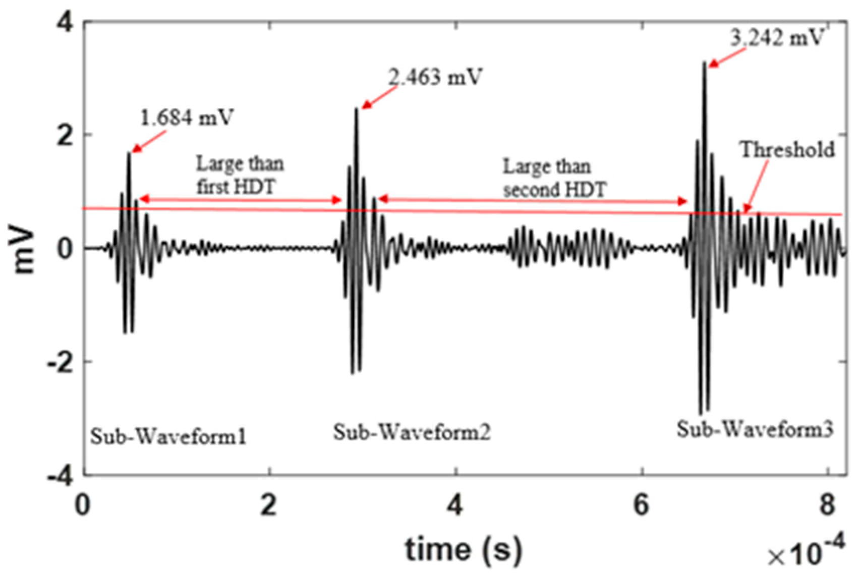
3.2.2. Performance Against Hit Definition Time

A realistic AE waveform generated in metal was used to evaluate the performance of AE entropy against the hit definition time (HDT) [39]. In this test, the same metal plate mentioned in the previous section was excited with a Vallen VS-900 AE transducer to generate elastic waves. The Vallen VS-900 transducer can be used both as an AE source and as a sensor. In this test, one AE transducer was used as a source to generate elastic waves and a second AE transducer was used as a sensor to measure the elastic waves.
Rectangular pulses with a very small width applied to the AE source transducer were used to generate the elastic waves. The rectangular pulsing pattern shown in Figure 6 was used to introduce a precise delay between each of rectangular pulses (i.e., 240 µs between the first and second pulses; 375 µs between the second and third pulses). The delay was used to separate the generation of an elastic wave in the plate, which supported the investigation into the influence of HDT in the recorded waveform. To vary the amplitude of the elastic wave in the plate, different heights of rectangular pulses were chosen (height of the first and second pulses were 0.5 and 0.75 times the third pulse). The elastic wave was captured as an analogue signal, with another AE sensor attached to the metal plate. The total distance between the transducer was 130 mm. Figure 7 illustrates the transducer arrangement used in the test. The narrow rectangular pulses act like PLB impulse excitation in the plate. Therefore, the frequency response of the elastic wave in the plate was not known prior to the experiment. The Vallen VS-900 was chosen as a transducer for both the pulsing and capturing of elastic wave as it was sensitive to a wide range of frequency and can successfully capture the true nature of the elastic wave. The transducers used in this experiment were the same as the one used as a sensor in the previous experiment (i.e., in Section 3.2.1). Figure 4 shows an image of the sensor and its frequency sensitivity spectrum.
The analogue signal captured by the sensor was passed on to three different channels in AMSY-6. Each channel acquired the signal with a different HDT than the other. Table 3 shows the range of HDTs used for this analysis. The rest of the acquisition settings were the same as the ones in Table 2. The traditional AE features for each channel were calculated by the AE data acquisition system, and AE entropy was calculated from the discrete voltage value using a MATL MATLABTM script written for this purpose. Finally, the influence of HDT on AE entropy was evaluated and compared with the traditional features.

3.2.3. Experimental Validation Procedure

In order to validate the proposed idea, AE entropy was calculated and explored from the waveforms recorded during tensile and fatigue loading of a standard 316L stainless steel sample. Table 4 shows the mechanical properties of the material used in this experiment. Flat tensile and fatigue specimens were designed according to ASTM standard E8/E8M–09 and E466-15, respectively [40,41]. Figure 8 shows the dimension of the specimens that were used in the experiment.
The tests were carried out on these specimens in an Instron servo hydraulic machine at room temperature (20 °C). The tensile sample was subjected to a displacement-controlled (1 mm/s) loading. The fatigue sample was subjected to sinusoidal loading of 5 Hz and maximum and minimum stress of 480 MPa and 48 MPa. For both the tests, the loading axis was parallel to the longitudinal direction of the material.
Elastic waves generated in the material were captured as analogue signals with two AE sensors (VS-160, manufactured by VallenTM [42]). This sensor was chosen because it has a higher peak sensitivity than the VS-900 at 160 kHz, which is close to the frequency of waveforms generated during yielding and crack initiation in austenitic stainless steel [14,22]. An illustration of this sensor and its frequency sensitivity spectrum is shown in Figure 9. The signals were amplified (using AEP4H amplifiers [43]). The amplified signals were fed to the AE data acquisition system (Vallen-AMSY-6). The analogue signals were sampled with a sampling frequency of 5 Mhz (larger than the ‘Nyquist frequency’ of waveform generated during damages in austenitic stainless steel [22]) in the AE data acquisition system. The window length of the recorded waveform was chosen to be 820 µs, which is comparable to the rise-time of typical sloshing impact on the primary wall [4]. The threshold chosen for these tests was 45 dB (i.e., above the background noise of the laboratory). The rest of the settings used in the AE data acquisition system were similar to the ones mentioned in Table 2. Due to the nature of fatigue loading, unwanted noise originating from the grips can mask the useful information in the dataset [44]. To avoid this, a 1D localization filtration technique was used, which considered signals generated within the gauge section of the specimen to be useful and avoided unwanted signals from the grips. All the recorded waveform features were calculated by the AE data acquisition system, and AE entropy was calculated by a MATLABTM coded algorithm (Appendix B) from the discrete values of the waveform.
To correlate the material behaviour with AE activity, the specimens were monitored simultaneously with a ARAMIS-5m digital image correlation (DIC) camera [45]. The material behaviour correlated for the tensile specimen was engineering stress and strain. The use of an extensometer is a traditional method to extract the strain in the material during tensile deformation. In this study, the deformation was expected to be quite large (since the material is very ductile), and there was a possibility of the extensometer scratching against the surface of the specimen during deformation. Scratching of the extensometer on the specimen surface was expected to generate unwanted elastic waves that can potentially corrupt the dataset. The DIC provided a noncontact strain measurement method and as a result the possibility of this noise in the specimen was avoided. For the fatigue specimen, the material behaviour such as the onset of plastic zone formation was correlated with AE activity. An image of the experimental setup for the tensile and fatigue test is shown in Figure 10 and Figure 11, respectively.

4. Experimental Results

4.1. Influence of Threshold on AE Entropy

The elastic wave in the metal plate as a result of PLB was acquired by six channels (refer to Figure 5 for the experimental setup). Each channel captured the elastic wave as a waveform with a different threshold than the others. The AE entropy and the traditional AE features for the same waveform acquired with different thresholds are shown in Figure 12. To understand the influence of threshold, a polynomial trend-line with an order of 4 has been added to all the graphs in Figure 12. It is evident from the graphs (Figure 12a,d) of this figure that as the acquisition threshold increases, traditional features (such as rise-time, duration, count and energy) extracted from the same waveform decrease. This is because the traditional feature extraction process is heavily dependent on the acquisition threshold. It is also obvious from Figure 12e,f that the peak amplitude and AE entropy do not show any variance with the acquisition threshold and are independent of it.
During AE monitoring, multiple elastic waves can be generated in a small timeframe from the activation of many damage sources. As a result, a waveform can contain information regarding many elastic waves (many damage sources) [20]. With a small threshold, traditional AE features are efficient in extracting the collective information in these waveforms. However, a higher threshold can compromise the feature extraction process and can bring difficulty in AE monitoring. Discrete voltage values collectively define the nature of the waveform; hence, its distribution is very crucial. Although the peak amplitude feature is independent of threshold, it does not take into account the collective information from the discrete voltage values. Therefore, it is not efficient in identifying the nature of the waveform. On the other hand, AE entropy is independent of acquisition threshold and its computation takes into account every discrete voltage value in a complete waveform, including the ones that are below the acquisition threshold. As a result, the collective information can be easily interpreted with AE entropy.

4.2. Influence of HDT on AE Entropy

The elastic wave in the metal plate (as a result of rectangular pulse excitation of an AE transducer) was captured with another AE sensor. The signal from the sensor was acquired by the AE data acquisition system three times with three different HDT settings. Figure 13 shows an acquired waveform for a HDT of 200 µs. In fixed window length settings, the distribution and the total number of the discrete voltage values in a waveform are not dependent on HDT. Hence, the three waveforms recorded with the three HDT’s are identical. It can be observed in Figure 13 that the entire waveform consists of three sub-waveforms. A waveform with multiple sub-waveforms was chosen for this analysis as it can appear when a material emits many elastic waves in a short interval. For instance, the cyclic plastic zone extension in austenitic stainless steel can generate a waveform containing two sub-waveforms [46]. It is also evident from Figure 13 that the peak of the first and second sub-waveform is 0.5 and 0.75 times the third waveform. This corresponds well with the amplitude of the excitation pattern used for this test.
The AE entropy and the traditional AE features for the waveform acquired with three HDT’s are shown in Figure 14. The Figure 14a–f represents the influence of HDT on rise-time, duration, count, energy, peak amplitude and AE entropy, respectively. Although the three waveforms are identical, as the HDT increases, the features extracted by the AE data acquisition also increases.
The first HDT setting has the lowest values of all the recorded feature. In this setting, AE features were only calculated from the first sub-waveform from the entire acquired waveform in Figure 13. This is because the duration from when the first sub-waveform dropped below 50 dB to the onset of the second sub-waveform was greater than the first HDT (200 µs). In AE, this phenomenon is termed as the expiration of HDT. Currently in AE monitoring, features are only extracted before the expiry of HDT, and the part of the waveform outside the HDT is discarded [39]. In the second HDT setting, AE features were calculated from the first and second sub-waveform. As a result, it had a higher value of duration, count and energy. It is also evident from Figure 14 that the rise-time and peak amplitude are also higher in the second HDT settings. This is because the peak voltage and its time of occurrence was calculated from within the first and second sub-waveform (the second sub-waveform had a higher peak voltage compared to the first one). The second HDT (300 µs) was greater than the duration from when the first sub-waveform dropped below 50 dB to the onset of the second sub-waveform. However, it was smaller than the duration from when the second sub-waveform dropped below 50 dB to the onset of the third sub-waveform. Therefore, the second HDT expired before the onset of the third sub-waveform. As a result, the feature was extracted over a larger duration compared to the first HDT setting. The third HDT (400 µs) was greater than the duration between each of the pairs of sub-waveforms in Figure 13 (first and second; second and third). Therefore, it did not expire between the sub-waveforms, and the AE features were calculated from the entire duration of the waveform. The AE feature for this HDT was the largest (including the peak amplitude and rise-time, since they were extracted from the third sub-waveform, which had the largest peak voltage).
It can be observed in Figure 14f that AE entropy shows no variance with HDT, unlike any other traditional AE feature. AE entropy is calculated from the distribution of the discrete voltage values. Since the distribution and total number of discrete voltage values remained identical between the three waveforms, they all yielded the same value of AE entropy. It is clear from this analysis that AE entropy is independent of HDT. As a result, the loss of information from the sub-waveforms occurring at different time intervals within the waveform can be avoided.

5. Validation and Discussion

5.1. Tensile Test

The material’s response during the test (such as stress and strain) was extracted from the sequence of DIC images taken for the entire length of the test (approximately 40 minutes). Figure 15 shows the reference DIC image and the strain evaluation points in the specimen. The correlation of traditional features and AE entropy of the AE events, captured with respect to the material response, from the tensile specimen is shown in Figure 16. Figure 16a–f represents the variance of rise-time, duration, count, energy, peak amplitude and AE entropy, respectively, for the entire range of deformation.
A number of researchers have concluded that during tensile deformation of austenitic stainless steel, there is remarkable AE activity in the initial stages of deformation [15,22]. This remarkable source of AE activity is attributed to the dislocation movement. It can be observed in all the graphs of Figure 16 that from the onset of loading up to about 0.044 strain, there is plenty of AE activity. Strain of 0.044 corresponds to an apparent plasticity in the specimen (as yielding is considered at 0.02 strain). Therefore, like the previously reported research, the initial increase in AE activity observed in all the graphs of Figure 16, can be attributed to the dislocation movement as a result of yielding. It can also be observed in all the graphs of Figure 16 that after the initial increase, there was no AE activity recorded until the fracture. It is mentioned in references [20,22] that as the austenitic stainless steel continues to deform after yielding, the glide distance of the dislocation movement decreases. Owing to this reason, the dislocation movement after significant yielding does not produce any detectable AE activity. A similar study in austenitic stainless steel concluded that failure in un-notched specimens of austenitic stainless steel occurs by extensive necking, which generates very little elastic wave [15,16,20]. It is evident from all the graphs in Figure 16 that at fracture, the AE activity was significantly lower as compared to the yielding. The occurrence of lower AE activity at fracture can therefore be attributed to the failure by extensive necking.
It can be noticed in Figure 16c–f that count, energy and peak amplitude exhibits the same trend as AE entropy. The fracture of metals is known to produce AE events with enhanced traditional AE features (e.g., count, energy and peak Amplitude) [44]. It is evident from these results that the fracture of the specimen had a dominant AE entropy like the traditional features. However, during yielding, there were no apparent distinguishable events. During yielding, AE entropy was distributed approximately between 0 and 8, whereas the fracture was accompanied by a value beyond 10. Count and peak amplitude has been widely used to study the failure mechanism in austenitic stainless steel during tensile deformation [14,15,17,20,22]. It is clear from these results that AE entropy exhibits the same trend as the count and peak amplitude. Therefore, it has the potential to replace them in a similar investigation. It can be observed in Figure 16a that during yielding, the rise-time of the AE events were distributed between 0 and 800 µs, whereas at fracture, it was noticeably lower. The rise-time feature does not provide much information of tensile deformation, and as a result, it has never been used to predict failure in these circumstances. It is also clear in Figure 16b that there was no distinguishable change in the duration of the events during fracture from yielding. A fixed window length setting (820 µs) limited the length of the waveform over which the duration was computed. As a result, there was no significant increase in duration of the events at fracture.

5.2. Fatigue Test

DIC enabled the correlation of the damage mechanism (i.e., the onset of plastic zone formation) with AE activity. The AE data and DIC images were synchronized by starting both measurements at the same time so that they capture data simultaneously. Figure 17 illustrates important DIC images of the strain map (εyy). Figure 17a represents the reference image. This image shows the state of the strain in the specimen before the onset of loading. Figure 17b shows that the strain maximizes in the middle of the specimen, and this image was taken after 1000 s from the start of loading. It is clear from Figure 17c, taken at 21556 s, and Figure 17b that there was no noticeable difference between them. This indicates that the surface strain from 1000 s to 21556 s remains stable. Figure 17d, taken at 22911s, shows the concentration of strain at the specimen edge, forming a plastic zone (indicated by an arrow). A significant formation and coalescence of a micro-crack may have resulted in this plastic zone. An explanation of this circumstances is provided in reference [47]. Figure 17e, taken at 23250 s, shows an enhancement of the plastic zone found in Figure 17d (indicated by an arrow). This plastic zone area becomes clearly highlighted in Figure 17f, taken at 23590 s (indicated by an arrow). Figure 17g, at 23928 s, shows a visible fatigue crack from the plastic zone seen in the earlier images. The time of occurrence of the plastic zone and fatigue crack is cross validated with AE activity.
The correlation of traditional features and AE entropy of the filtered events, captured from the fatigue specimen, is shown in Figure 18. Figure 18a–f represents the variance of rise-time, duration, count, energy, peak amplitude and AE entropy for the entire length of the test. It is evident from Figure 18c–f that at the initial and final stage (at the beginning and end of the test), there was a significant increase in count, energy, peak amplitude and AE entropy. The initial and final stage was accompanied with an AE entropy above 10.
The initial increase in these traditional features and AE entropy is due to the rapid yielding (i.e., caused by the onset of loading). The maximum engineering stress exerted on the specimen at each cycle of loading (including the first cycle) was 480 MPa. This is beyond the yield stress of the material. As a result, yielding was introduced in the specimen in the first cycle of loading. Yielding in austenitic stainless steel has been reported to be accompanied by the sharp increase in some traditional AE features (e.g., count and peak amplitude). The increase in the traditional features and AE entropy at the final stage is due to the fracture of the specimen. It is clear from these results that like the traditional features, AE entropy is also sensitive to the yielding and fracture of austenitic stainless steel.
It is a well-known fact that fatigue crack initiation leads to plastic zone formation in the specimen, and the crack propagates until the final fracture [48]. The DIC, as a secondary monitoring technique used in this test, was able to identify the onset of plastic zone formation. The onset of plastic zone formation in the specimen, identified by DIC, is marked with a red dashed line in each of the graphs of Figure 18. It can be observed in Figure 18c–f that there was no noticeable increase in count, energy, peak amplitude and AE entropy at the onset of plastic zone formation. In fact, apart from yielding and fracture, there was no noticeable increase in these traditional AE features and in AE entropy.
The plastic zone is known to produce continuous AE waveforms with higher rise-time [49]. Therefore, the noticeable increase in rise-time (Figure 18a) at around the red dashed line could be from the plastic zone. It can be observed Figure 18b that the duration of the events did not show any trend. The duration of events during the initial yielding and final fracture was expected to be higher (since these events had a higher peak amplitude). However, no distinct increase in duration could be observed during these stages. The fixed window length settings (820 µs) used for this test masked the performance of duration.
Research on fatigue damages using AE are mostly conducted by analysing the cumulative trend of count and energy [46,48,50,51]. Therefore, in order to further evaluate the performance of AE entropy, its cumulative trend was compared with the traditional features in Figure 19.
It can be observed in Figure 19 that in the beginning of the test, there was a small increase, and at the end, there was a significant increase in the cumulative energy. The increase in the cumulative energy in the beginning is attributed to the yielding as a result of the onset of loading, whereas the significant increase in the cumulative energy at the end is due to fracture of the specimen. The plastic zone identified by DIC for this test was at 22,911 seconds. However, there was no significant change observed in the cumulative energy at that time. In fact, in the period between the yielding and fracture of the specimen, there was no noticeable increase in the cumulative energy. Highly energetic AE events towards the end may have masked the cumulative trend in energy between yielding and fracture.
It is clear from Figure 19 that the cumulative entropy exhibits the same trend as the cumulative count for the entire duration of the test. At around 23,000 s, a significant jump could be noticed in both the cumulative features. This time corresponds to the plastic zone formation in Figure 17. Hence, it can be concluded that the noticeable jump in the cumulative AE entropy and count is an indication of the formation of the plastic zone. It is also evident from Figure 19 that there was a noticeable increase in the cumulative AE entropy and count after 20,000 s. However, DIC images in Figure 17 only shows a noticeable change in the strain map from 21,556 s onwards. Therefore, the noticeable increase in the cumulative AE entropy and count, from 20,000 s, could be a result of the growth and coalescence of micro-cracks, which is not reflected in DIC results.

5.3. Correlation Between the Coupon Specimen and Real Structures under Operation

In a LNG cargo tank, sloshing is the only unpredictive load that results in its structural degradation. Sloshing studies conducted in accordance with the American Bureau of Shipping and DVN.GL guidelines suggest that the maximum and mean duration of the sloshing impact were 200 ms and 11.7–27.4 ms, respectively [29,52]. It is also suggested in reference [52] that the sloshing impacts are separated by zero pressure intervals in the order of a few seconds, and the interval between the sloshing impacts are not consistent. Figure 20 shows the loading spectra adopted in fatigue testing of this research. The specimens were subjected to the same loading spectra from the start of the test until fracture. It is evident from this figure that the duration of the respective load (i.e., from one minimum load point to the next) was 200 ms, which is comparable to the maximum duration of the sloshing impact experienced by a LNG cargo tank during voyage. However, it can be observed from this figure that there was no delay between the subsequent load. In other words, there was no separation between the subsequent loads, as experienced by the real LNG cargo tank.
Despite the potential of cumulative AE entropy in providing valuable information of damage (i.e., plastic zone formation) discovered during fatigue tests of this study, it cannot be implemented as a condition-monitoring technique on the primary wall of the cargo tank. This is primarily because the loading condition of the coupon specimen adopted in this study was continuous in nature without any delay between the subsequent load. Hence, there may not be a noticeable increase in the cumulative AE entropy, during plastic zone formation especially, if the duration of zero pressure intervals between sloshing impact increases during plastic zone formation as compared to the other stages.
Considering that the cumulative AE analysis may not be a suitable condition monitoring technique for the primary wall, the only other technique that can be explored is the correlation analysis of AE features. It can be observed in Figure 18f that during the onset of plastic zone formation, there was no noticeable increase in AE entropy. In fact, it can be observed in Figure 18c–e that there was no noticeable increase in either count, energy or peak amplitude at the onset of plastic zone formation. It is mentioned in reference [53], that the rate of AE activity increases with the formation and growth of the plastic zone. However, the correlation AE analysis (e.g., count, energy, peak amplitude and AE entropy) did not provide any information regarding the formation of the plastic zone. This indicates that although the rate of AE event generation was higher, the individual strength of AE events did not change noticeably. In austenitic stainless steel, plastic zone formation is known to produce AE events with weaker features as compared to the ones at fracture [46]. This is because the amount of material yielding in and at the edge of plastic zone is not sufficient to produce AE events with high strength. Since the AE entropy during the formation of plastic zone is lower as compared to the ones at fracture and onset of yielding, it suggests that AE events during these periods are less disordered. It can also be suggested that the lower strength AE events during this period is responsible for its low disorderness. It is clear that the plastic zone formation due to repeated cyclic loading will not be identified by AE entropy and traditional features. The plastic zone precedes crack initiation in material subjected to fatigue loading. Since the AE entropy is not sensitive to plastic zone formation, a warning prior to the crack initiation in the primary wall of the cargo tank cannot be successfully achieved.
It is clear in Figure 18f that the initial yielding (at the onset of loading) was associated with a noticeable increase in AE entropy. Like the AE entropy, it can be observed in Figure 18c–e that during the initial yielding, there was also a noticeable increase in the traditional AE features (e.g., count, energy and peak amplitude). The yielding/deformation activities in the primary wall of the cargo tank, due to single sloshing impact are an important source of information as they are considered to be a dominant damage mechanism during voyages [54,55]. Since AE entropy is capable of providing a noticeable indication during yielding, it can be successfully applied to monitor the primary wall against this damage mechanism. The information of yielding/deformation in the primary wall can educate the ship operators regarding the structural condition of the cargo tank so that appropriate maintenance can be planned to avoid further failure and shut down costs.
It can be observed from Figure 16c–f that the yielding in tensile test was not accompanied by a noticeable increase in AE entropy and the traditional features (e.g., count, energy and peak amplitude), unlike in the fatigue test. This difference in AE behaviour between the tensile and fatigue specimen arises due to their respective loading conditions. The tensile specimen was subjected to a constant strain rate of 0.0040 or 1 mm/s from start of the test until fracture whereas the fatigue specimen was subjected to a strain rate of 0.157 during the initial yielding (due to the onset of loading). In comparison to the loading at a constant strain rate during tensile test, the strain rate at the onset of yielding in fatigue test was significantly higher.
Strain rate has been shown to enhance the AE events generation in a wide range of materials such as α brass [56], 7075-T6 aluminium [57], discontinuous yielding material [58], single crystal copper [59] and austenitic stainless steel [20,22]. For instance, in α brass, the count of AE events increases with the strain rate [56]. In 7075-T6 aluminium [57], the root mean square (RMS) voltage of AE events was proportional to the strain rate. The increase in strain rate on single crystal copper was accompanied by an increase in count and RMS voltage of AE events [59]. In austenitic stainless steel [20,22], with the increase in strain rate, the RMS voltage, count and frequency content of the AE events has been shown to increase. The increase in AE event generation, in all these studies, was attributed to the increase in rate of source activation instead of the formation of the new source. In austenitic stainless steel, this increased rate of source activation refers to the increase in velocity of the mobile dislocation [22]. In other words, with the strain rate, the velocity of the mobile dislocation also increases. It has been reported in references [20,60] that the strain rate in austenitic stainless steel is related to the mobile dislocation velocity according to Equation (3):
e = p m b v a v
where e is strain rate, pm is the dislocation density, b is the Burgers vector and vav is the average dislocation velocity. It has also been reported in reference [61] that the squared RMS voltage of the AE waveform recorded during deformation is directly proportional to the strain rate in many single and poly crystals. The relation between the strain rate and RMS voltage, according to this study is shown in Equation (4), where e is the strain rate, Vrms is the RMS voltage and t is the window length of the waveform.
t × V R M S 2 e
Thus, from Equations (3) and (4), it can also be deduced that the voltage RMS is related to the dislocation density pm, the Burgers vector b and the average dislocation velocity vav. The equation relating these quantities is shown in Equation (5). By considering this relation, it is suggested in reference [22] that in austenitic stainless steel, with the increase in average velocity of the dislocation (due to higher strain rate), the Vrms of the waveform also increases.
V r m s 2 = p m b v a v
Therefore, it can be suggested that the higher strain rate of the fatigue test during yielding resulted in the generation of waveform with larger Vrms, which in turn resulted in the noticeable increase in AE entropy. In the cargo tank, the maximum duration of sloshing impact is 200 ms, which is identical to the duration of respective load in fatigue test. Owing to this reason, a strong sloshing impact has the potential to cause deformation in the primary wall with a significantly higher strain rate (comparable to the one in the fatigue test) than the standard tensile test of this research. Therefore, the deformation in the primary wall due to sloshing can be associated with a noticeable increase in AE features. AE entropy in particular can be expected to be above 10 during the deformation caused by sloshing.

5.4. Effect of Noise on AE Eentropy

It is worth noting that the waveforms of each event may contain some noise. This noise is impossible to filter out with the traditional AE filtration techniques (e.g., 1D localization) [44,46,50,62,63,64,65], as they are embedded in the waveform. The presence of noise in the waveform can affect the disorderness of the discrete probability distribution. Therefore, it has the potential to influence the calculated value of AE entropy from a waveform. Like the AE entropy, noise in the waveform can also influence the traditional AE features.
In order to eliminate the noise embedded in the AE waveform, a few studies have proposed a signal processing approach [66,67,68]. These studies are based on de-noising (e.g., conditioning) the AE waveform with discrete wavelet transform (DWT) prior to extracting the features. These studies suggest that DWT is very effective in reducing the noise in a waveform. Hence, this technique was adopted in this study to investigate the effect of de-noising a waveform to calculate its AE entropy. De-noising using DWT is based on the wavelet theory. In this approach, a series of wavelet is used to obtain the wavelet coefficient of the signal to be de-noised. The series of wavelets is generated by scaling and translating a mother wavelet. The wavelet coefficients obtained are referred to as the DWT (a,b), which is a function of the translating b with a fixed scale factor a. The DWT helps analyse the waveform at a different level of frequencies by decomposing it to several level approximations and details.
The procedure for waveform de-noising using DWT is accomplished with three steps. Firstly, the waveform is decomposed into several levels using a series of wavelet from a mother wavelet. Each level contains approximation coefficients representing the low pass filter and a detail coefficient representing a high pass filter. Secondly, thresholding is carried out on every detail coefficient using a threshold rule (e.g., minimax, Heursure, sqtwolog, SURE), in conjunction with a hard or a soft thresholding. Finally, the signal is reconstructed by inverse DWT from the updated detail coefficient on every level and updated approximation coefficient on the final level. In this research, db8 was chosen as the mother wavelet [69], decomposition level was chosen to be 8 and a soft thresholding method was implemented. These parameters were chosen as they yielded the best de-noising performance of the AE waveform among many other set of de-noising parameters [67].
Figure 21a,b illustrates the original and de-noised waveform of two AE events. The AE entropy of the original waveform was 10.3 and 10.5, respectively, whereas that of the de-noised waveform was 8.7 and 8.4, respectively. It is clear from this analysis that de-noising the waveform reduces the AE entropy slightly. This is because de-noising procedure decreases the disorderness in the probability distribution of the waveform. It is also evident that despite the presence of noise, the majority of the disorderness in the original waveform arises form microstructural changes in the material (as de-noising only slightly reduces the AE entropy). As a result, there is no need to perform the de-noising when AE entropy is used for damage monitoring.

6. Conclusions

This research addresses one of the major drawbacks of the state-of-the-art AE monitoring technique and improves it so that the possibility of AE implementation for monitoring the primary wall is increased. The improved technique is based on an AE feature, which is a measure of randomness of the AE waveform, calculated using Renyi’s entropy. The new technique is referred to as AE entropy in this research. AE entropy reduces human involvement with the data acquisition system and has the potential to be implemented in the commercial AE data acquisition system. The following points summarise the key findings of this study:
  • The evaluation process adopted in this study suggests that AE entropy is independent of user-defined acquisition threshold and extracts the collective information from a waveform. This independency of AE entropy arises as it is directly calculated from the discrete voltage values, which are both in and outside the threshold.
  • The evaluation process also suggests that AE entropy is independent of the user defined HDT. This is mainly because the computation of AE entropy takes into account the discrete voltage values in a waveform even after the expiration of HDT. This independency of AE entropy is an important property, as the loss of information from sub-waveforms occurring at different time intervals within a waveform can be avoided.
  • In the tensile test, correlation AE entropy possessed the same trend as most of the widely used traditional AE features. From the onset of loading to just after yielding, there was plenty of AE activity due to dislocation movement; however, it did not have dominant AE entropy, whereas the fracture of the specimen was accompanied by a small number of AE activities, but it had dominant AE entropy.
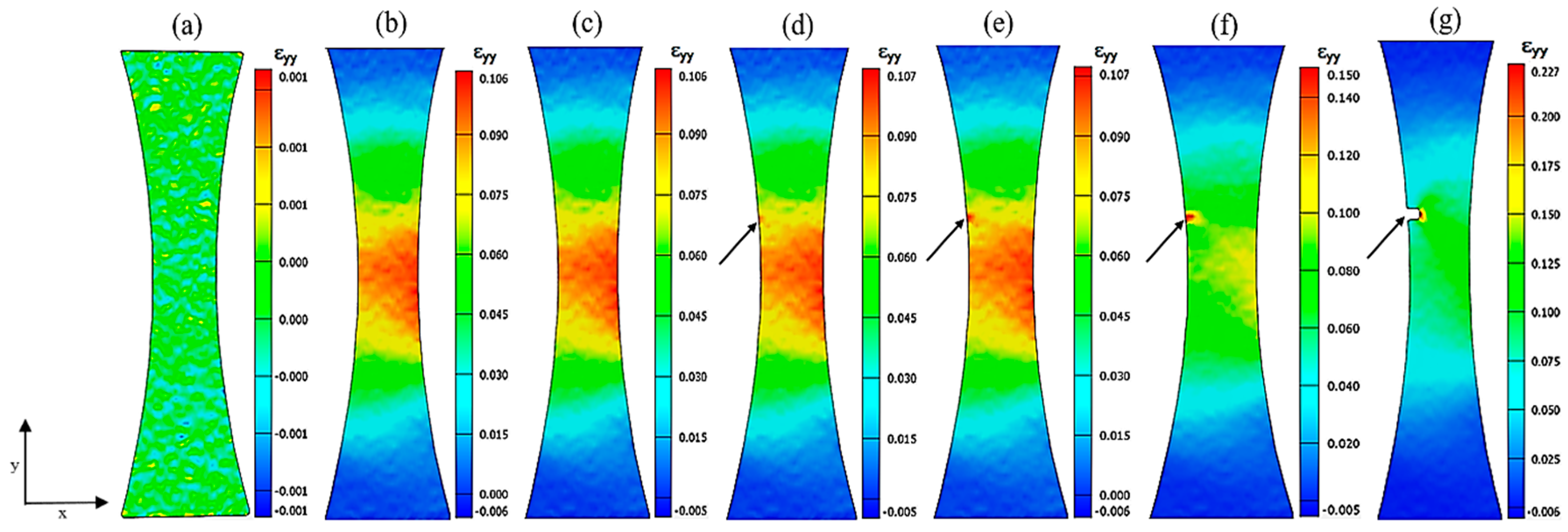
  • In the fatigue test, the yielding was accompanied by a dominant increase in correlation AE entropy. This suggests that AE entropy has the potential to provide indication regarding the yielding, which is considered to be a dominant damage mechanism in the primary wall. Since AE entropy is sensitive to yielding, it can be successfully implemented to monitor the primary wall against this damage mechanism. At the formation of plastic zone (identified by DIC), there is no noticeable increase in the AE entropy. This suggests that it may not be a suitable technique for the identification of plastic zones formed due to repeated cyclic loading.
  • Compared to the yielding of the tensile specimen, the yielding of fatigue specimen was accompanied by dominant correlation AE entropy. This was due to an enhanced average velocity of the moving dislocation (vav), as a result of the higher strain rate (e) of fatigue specimens. Duration of the cyclic loading adopted in this study was comparable to the duration of the sloshing impact. Therefore, a strong sloshing impact has the potential to cause deformation in the primary wall with a high strain rate (than that of the strain rate of tensile test), which can produce dominant AE entropy.
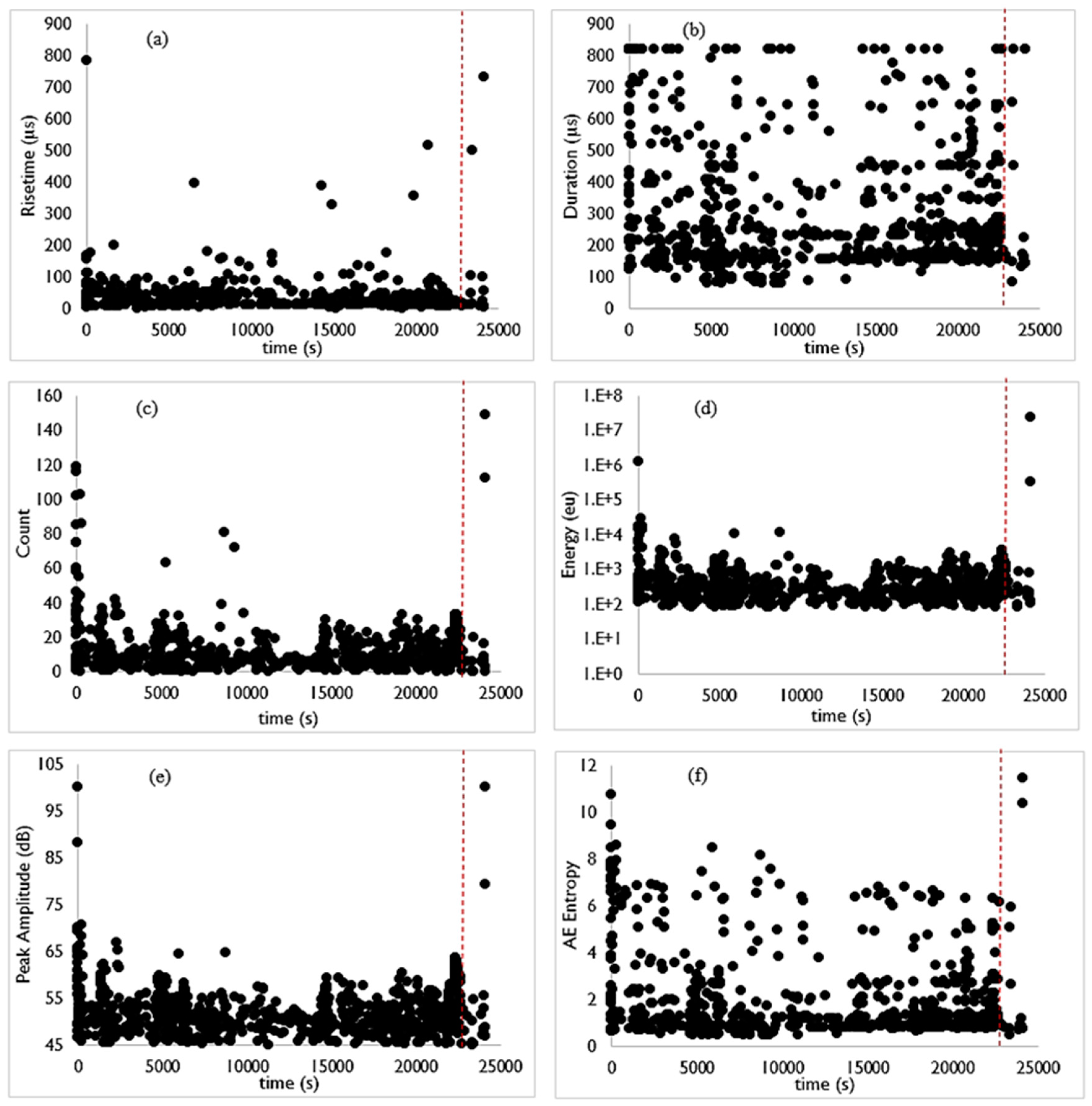
  • Both the cumulative count and AE entropy increased noticeably before the damage manifests into plastic zone formation. At the formation of a plastic zone (identified by DIC), there was a sharp increase in both of these cumulative features. A similar trend in these cumulative features suggest that the traditional analysis of cumulative count can be replaced with cumulative AE entropy in the experimental investigation of fatigue damage evaluation. Despite the potential of cumulative AE entropy to identify the fatigue damage evolution, it cannot be used to monitor the primary wall primarily because the sloshing impact on the primary wall is separated by zero pressure intervals. As a result, there might not be a noticeable change in the cumulative feature if the duration of zero pressure values increase during plastic zone formation.
  • The majority of the disorderness in a waveform arises from micro-structural damage. As a result, there is no need to perform the de-noising of the waveform prior to the calculation of AE entropy.
AE entropy provided the same information as the traditional AE features in our laboratory-based experiments. However, before it can be successfully implemented to monitor the primary wall of LNG tanks, further theoretical and experimental work is required. Firstly, the nature of noise in the primary wall during service operation needs to be understood so that an effective filtration of the AE data can be carried out. Secondly, the performance of AE entropy in a noisier environment needs to be assessed. Finally, to avoid the effect of attenuation on the AE entropy there has to be an optimum network of sensors deployed on the primary wall to effectively capture elastic waves from any part of the tank where damage is occurring. This can only be achieved by having a clear understanding of the attenuation of elastic waves in the primary wall.

Author Contributions

Conceptualization, F.T.S. and T.P.S.; methodology, F.T.S.; software, G.E.; validation, F.T.S. and G.E.; formal analysis, F.T.S.; investigation, F.T.S. and G.E.; resources, T.P.S.; data curation, F.T.S.; writing—original draft preparation, F.T.S.; writing—editing, T.P.S. and G.E.; visualization, T.P.S.; supervision, T.P.S. and G.E.; project administration, F.T.S.; funding acquisition, G.E.

Funding

This work was funded in part by Lloyds Register Foundation, in part by London South Bank University, in part by TWI Ltd, and in part by National Structural Integrity Research Centre.

Conflicts of Interest

The authors declare no conflict of interest.

Appendix A

Entropy of a variable is the average number of bits needed to represent the variable. According to Kolmogorov’s theory, the average of variable {x1, x2, x3, …, xn}, is represented using Equation (A1).
M e a n = g 1 i = 1 n [ w ( x i ) g ( x i ) ]
where:
  • w ( x i ) represent the weight of the variable, such that i = 1 n w ( x i ) = 1 ;
  • g ( x ) is a strictly continuous monotonic function and g 1 ( x ) is its inverse function. For arithmetic mean g ( x ) = x and g 1 ( x ) = x .
When Kolmogorov’s theory is used to determine the average or the arithmetic mean number of bit needed to represent a variable, Equation (A1) takes the form as shown in Equation (A2).
M e a n = g 1 k = 1 m [ P ( x k ) g ( log ( 1 P ( x k ) ) ]
where:
  • P ( x k ) represents the discrete probability distribution of the voltage values with the kth number of bin;
  • m represents the total number of bins;
  • log ( 1 P ( x k ) ) represents the number of bits need to represent the variable x k .
Since, g ( x ) (i.e., g ( log P ( x k ) ) in Equation (A2)) is a strictly continuous monotonic function, Renyi proved that it has two solutions. The first solution is g ( x ) = a x (i.e., g ( log P ( x k ) ) = a log P ( x k ) for Equation (A2)), with a 0 . Substituting the first solution in Equation (A2) yields Shannon’s entropy. Shannon’s entropy is the average number of bits required to represent a variable; in other words, it is the arithmetic mean of the total number of bits. The second solution is g a ( x ) = 2 ( a 1 ) x (or g a ( log P ( x k ) ) = 2 ( a 1 ) log P ( x k ) for Equation (A2). Substituting the second solution in Equation (4) results in Renyi’s entropy. Renyi’s entropy is considered to be an exponential mean of the total number of bits. Both Renyi’s and Shannon’s entropy can be defined with five sets of postulates. The first four postulates are common between both the entropy measures. However, they differ in their fifth postulates as a result of the choice of g ( x ) . In contrast to Shannon’s entropy, Renyi’s entropy has an additional term ‘a’ in the equation. The term ‘a’ in Renyi’s entropy appears as a power of the discrete probability distribution. As a result, the choice of ‘a’ makes Renyi’s entropy unique.
In order to investigate the performance of Shannon’s and quadratic Renyi’s entropy in terms of their sensitivity to disorderness, a decaying sinusoidal waveform (shown in Figure A1) and its corresponding signal-to-noise ratio (SNR) of 10, 20, 30 and 40 were analysed. The waveform in Figure A1 is considered to be highly ordered compared to its corresponding SNR. Therefore, the difference in the respective entropy measurement techniques (e.g., Shannon’s and quadratic Renyi’s) between the waveform in Figure A1 and its corresponding SNR should provide a true measure of performance against capturing the disorderness. Figure A2 shows the delta entropy against SNR for both Shannon’s and quadratic Renyi’s entropy. The delta entropy corresponds to the difference in the entropy between waveform A1 and its corresponding SNR.
It can be observed in this graph that for each of the SNR, the delta entropy for quadratic Renyi’s entropy is noticeably higher than that of Shannon’s entropy. In other words, the spread in data between the ordered and disordered waveform will be much higher for quadratic Renyi’s entropy compared to that of Shannon’s entropy. Therefore, it can be concluded that quadratic Renyi’s entropy is much more efficient in capturing the disorderness, which is an indication of disorderness.
Figure A1. Decaying sinusoidal waveform.
Applsci 09 04070 g0a1
Figure A2. Delta entropy against signal-to-noise ratio (SNR) for Shannon’s and Renyi’s entropy.
Applsci 09 04070 g0a2

Appendix B

Bins = −100:0.00305:100;
[h,bins] = hist(vecTR,bins);
H = h’;
A = bins’;
P = H./sum(H);
A = sum(p.^2);
H2(X) = −log2(A)

References

  1. International Gas Union. World LNG Report; International Gas Union: Barcelona, Spain, 2018. [Google Scholar]
  2. Ryu, M.C.; Jung, H.; Kim, Y.S.; Kim, Y. Sloshing design load prediction of a membrane type LNG cargo containment system with two-row tank arrangement in offshore applications. Int. J. Nav. Archit. Ocean Eng. 2016, 8, 537–553. [Google Scholar] [CrossRef] [Green Version]
  3. Oh, M.-C.; Seo, J.-K.; Kim, K.-J.; Lee, S.-M.; Kim, M.-H. In Situ Measurement of Sloshing Impact on LNG Insulation Panel by using High Speed Fiber Optics. J. Intell. Mater. Syst. Struct. 2010, 21, 787–796. [Google Scholar] [CrossRef]
  4. Graczyk, M.; Moan, T.; Wu, M. Extreme sloshing and whipping-induced pressures and structural response in membrane LNG tanks Extreme sloshing and whipping-induced pressures and structural response in membrane LNG tanks. Ships Offshore Struct. 2007, 2, 201–216. [Google Scholar] [CrossRef]
  5. Park, J.-J.; Kim, S.-Y.; Kim, Y.; Seo, J.-H.; Jin, C.-H.; Joh, K.-H.; Kim, B.-W.; Suh, Y.-S. Study on tank shape for sloshing assessment of LNG vessels under unrestricted filling operation. J. Mar. Sci. Technol. 2015, 20, 640–651. [Google Scholar] [CrossRef]
  6. Lee, H.B.; Park, B.J.; Rhee, S.H.; Bae, J.H.; Lee, K.W.; Jeong, W.J. Liquefied natural gas flow in the insulation wall of a cargo containment system and its evaporation. Appl. Therm. Eng. J. 2011, 31, 2605–2615. [Google Scholar] [CrossRef]
  7. Sohn, J.; Bae, D.; Bae, S.; Paik, J. Nonlinear structural behaviour of membrane-type LNG carrier cargo containment systems under impact pressure loads at −163 °C. Ships Offshore Struct. 2016, 12, 722–733. [Google Scholar] [CrossRef]
  8. Choi, S.W.; Kim, H.S.; Lee, W.I. Analysis of leaked LNG flow and consequent thermal effect for safety in LNG cargo containment system. Ocean Eng. 2016, 113, 276–294. [Google Scholar] [CrossRef]
  9. Han, S. Assessing Structural Safety of Inner Hull Structure Under Cryogenic Temperature. In Proceedings of the ASME 2011 30th International Conference on Ocean, Offshore and Arctic Engineering, Rotterdam, The Netherlands, 19–24 June 2011; pp. 1–7. [Google Scholar]
  10. International Maritime Organization. Resolution MSC.370(93) (Adopted on 22 May 2014); International Maritime Organization: London, UK, 2015.
  11. Gavory, T.; De Seze, P.E. Sloshing in membrane LNG carriers and its consequences from a designer’s perspective. In Proceedings of the Nineteenth International Offshore and Polar Engineering Conference, Osaka, Japan, 21–26 June 2009. [Google Scholar]
  12. Gowid, S.; Dixon, R.; Ghani, S. Profitability, reliability and condition based monitoring of LNG floating platforms: A review. J. Nat. Gas Sci. Eng. 2015, 27, 1495–1511. [Google Scholar] [CrossRef] [Green Version]
  13. Hellier, C. Handbook of Nondestructive Evaluation; McGraw-Hill: New York, NY, USA, 2013. [Google Scholar]
  14. Moorthy, V.; Jayakumar, T.; Raj, B. Acoustic emission technique for detecting micro- and macroyielding in solution-annealed AISI Type 316 austenitic stainless steel. Int. J. Press. Vessel. Pip. 1995, 64, 161–168. [Google Scholar] [CrossRef]
  15. Mukhopadhyay, C.K.; Ray, K.K.; Jayakumar, T.; Raj, B. Acoustic emission from tensile deformation of unnotched and notched specimens of AISI type 304 stainless steels. Mater. Sci. Eng. A 1998, 255, 98–106. [Google Scholar] [CrossRef]
  16. Mukhopadhyay, C.K.; Jayakumar, T.; Raj, B.; Ray, K.K. The influence of notch on the acoustic emission generated during tensile testing of nuclear grade AISI type 304 stainless steel. Mater. Sci. Eng. A 2000, 276, 83–90. [Google Scholar] [CrossRef]
  17. Mukhopadhyay, C.K.; Jayakumar, T.; Raj, B.; Ray, K.K. Acoustic emission-stress intensity factor relations for tensile deformation of notched specimens of AISI type 304 stainless steel. Mater. Sci. Eng. A 2000, 293, 137–145. [Google Scholar] [CrossRef]
  18. Mukhopadhyay, C.K.; Jayakumar, T.; Raj, B.; Ray, K.K. Acoustic emission during tensile deformation of pre-strained nuclear grade AISI type 304 stainless steel in the unnotched and notched conditions. J. Mater. Sci. 2007, 42, 5647–5656. [Google Scholar] [CrossRef]
  19. Mukhopadhyay, C.K.; Kasiviswanathan, K.V.; Jayakumar, T.; Raj, B. Acoustic emission during tensile deformation of annealed and cold-worked AISI type 304 austenitic stainless steel. J. Mater. Sci. 1993, 28, 145–154. [Google Scholar] [CrossRef]
  20. Venkataraman, B.; Mukhopadhyay, C.K.; Raj, B. Effect of variation of strain rate on thermal and acoustic emission during tensile deformation of nuclear grade AISI type 316 stainless steel. Mater. Sci. Technol. 2004, 20, 1310–1316. [Google Scholar] [CrossRef]
  21. Barat, K.; Bar, H.N.; Mandal, D.; Roy, H.; Sivaprasad, S.; Tarafder, S. Low temperature tensile deformation and acoustic emission signal characteristics of AISI 304LN stainless steel. Mater. Sci. Eng. A 2014, 597, 37–45. [Google Scholar] [CrossRef]
  22. Haneef, T.; Lahiri, B.B.; Bagavathiappan, S.; Mukhopadhyay, C.K.; Philip, J.; Rao, B.P.C.; Jayakumar, T. Study of the tensile behavior of AISI type 316 stainless steel using acoustic emission and infrared thermography techniques. Integr. Med. Res. 2015, 4, 241–253. [Google Scholar] [CrossRef] [Green Version]
  23. Máthis, K.; Prchal, D.; Novotny´b, R.; Novotny´b, N.; Hähner, P. Acoustic emission monitoring of slow strain rate tensile tests of 304L stainless steel in supercritical water environment. Corros. Sci. 2011, 53, 59–63. [Google Scholar] [CrossRef]
  24. Raj, B. Acoustic Emission Technique for Characterizing Deformation and Fatigue Crack Growth in Austenitic Stainless Steels. AIP Conf. Proc. 2003, 22, 1439–1446. [Google Scholar]
  25. Carpinteri, A.; Lacidogna, G.; Pugno, N. Structural damage diagnosis and life-time assessment by acoustic emission monitoring. Eng. Fract. Mech. 2007, 74, 273–289. [Google Scholar] [CrossRef]
  26. Carpinteri, A.; Xu, J.; Lacidogna, G.; Manuello, A. Reliable onset time determination and source location of acoustic emissions in concrete structures. Cem. Concr. Compos. 2012, 34, 529–537. [Google Scholar] [CrossRef]
  27. Anzani, A.; Binda, L.; Carpinteri, A.; Lacidogna, G.; Manuello, A. Evaluation of the repair on multiple leaf stone masonry by acoustic emission. Mater. Struct. Constr. 2008, 41, 1169–1189. [Google Scholar] [CrossRef]
  28. Kiesewetter, N.; Schiller, P. The acoustic emission from moving dislocations in aluminium. Phys. Status Solidi 1976, 38, 569–576. [Google Scholar] [CrossRef]
  29. Lee, S.E.; Kim, B.J.; Seo, J.K.; Ha, Y.C.; Matsumoto, T.; Byeon, S.H.; Paik, J.K. Toshiyuki Matsumoto. Nonlinear impact response analysis of LNG FPSO cargo tank structures under sloshing loads. Ships Offshore Struct. 2015, 10, 510–532. [Google Scholar]
  30. Hartley, R.V.L. Transmission Information. Bell Syst. Tech. J. 1928, 7, 535–563. [Google Scholar] [CrossRef]
  31. Shannon, C.E. A Mathematical Theory of Communication. Bell Syst. Tech. J. 1948, 27, 623–656. [Google Scholar] [CrossRef]
  32. Renyi, A. On measures of entropy and information. In Proceedings of the Fourth Berkeley Symposium on Mathematical Statistics and Probability, Berkeley, CA, USA, 20 June–30 July 1960; Volume 1, pp. 457–561. [Google Scholar]
  33. Cornforth, D.J.; Tarvainen, M.P.; Jelinek, H.F. How to Calculate Renyi Entropy from Heart Rate Variability, and Why it Matters for Detecting Cardiac Autonomic Neuropathy. Front. Bioeng. Biotechnol. 2014, 2, 34. [Google Scholar] [CrossRef]
  34. Coles, P.J.; Berta, M.; Tomamichel, M.; Wehner, S. Entropic uncertainty relations and their applications. Rev. Mod. Phys. 2017, 89, 015002. [Google Scholar] [CrossRef] [Green Version]
  35. Vinga, S.; Almeida, J.S. Rényi continuous entropy of DNA sequences. J. Theor. Biol. 2004, 231, 377–388. [Google Scholar] [CrossRef]
  36. ASTM. ASTM E976-15 Standard Guide for Determining the Reproducibility of Acoustic Emission Sensor Response; ASTM: West Conshohocken, PA, USA, 2015. [Google Scholar]
  37. AE-Sensor Data Sheet VS900-RIC. Available online: http://www.vallen.de/quote-ref (accessed on 11 July 2019).
  38. AMSY-6 System Description. 2015. Available online: http://www.vallen.de (accessed on 11 July 2019).
  39. Moradian, Z.; Li, B.Q. Hit-based acoustic emission monitoring of rock fractures: Challenges and solutions. Springer Proc. Phys. 2017, 179, 357–370. [Google Scholar]
  40. ASTM. ASTM E8M-13a-Standard Test Methods for Tension Testing of Metallic Materials; ASTM: West Conshohocken, PA, USA, 2009. [Google Scholar]
  41. ASTM. ASTM E466-15, Practice for Conducting Force Controlled Constant Amplitude Axial Fatigue Tests of Metallic Materials; ASTM: West Conshohocken, PA, USA, 2015. [Google Scholar]
  42. AE-Sensor Data Sheet VS160-NS. Available online: http://www.vallen.de/quote-ref (accessed on 11 July 2019).
  43. Acoustic Emission Preamplifiers Specification. 2017. Available online: http://www.vallen (accessed on 11 July 2019).
  44. Barsoum, F.F.; Suleman, J.; Korcak, A.; Hill, E.V.K. Acoustic emission monitoring and fatigue life prediction in axially loaded notched steel specimen. J. Acoust. Emiss. 2009, 27, 40–63. [Google Scholar]
  45. ARAMIS 3D Camera | GOM. Available online: https://www.gom.com/metrology-systems/aramis/aramis-3d-camera.html (accessed on 11 July 2019).
  46. Chai, M.; Zhang, J.; Zhang, Z.; Duan, Q.; Cheng, G. Acoustic emission studies for characterization of fatigue crack growth in 316LN stainless steel and welds. Appl. Acoust. 2017, 126, 101–113. [Google Scholar] [CrossRef]
  47. Sangid, M.D. The physics of fatigue crack initiation. Int. J. Fatigue 2013, 57, 58–72. [Google Scholar] [CrossRef]
  48. Fang, D.; Berkovits, A. Fatigue design model dased on damage mechanism revealed by acoustic emission measurement. ASME J. Eng. Mater. Technol. 1995, 117, 200–208. [Google Scholar] [CrossRef]
  49. Ono, K.; Cho, H.; Takuma, M. The origin of continuous emissions. J. Acoust. Emiss. 2005, 23, 206–214. [Google Scholar]
  50. Han, Z.; Luo, H.; Cao, J.; Wang, H. Acoustic emission during fatigue crack propagation in a micro-alloyed steel and welds. Mater. Sci. Eng. A 2011, 528, 7751–7756. [Google Scholar] [CrossRef]
  51. Amer, A.O.; Gloanec, A.L.; Courtin, S.; Touze, C. Characterization of fatigue damage in 304L steel by an acoustic emission method. Procedia Eng. 2013, 66, 651–660. [Google Scholar] [CrossRef]
  52. Graczyk, M.; Moan, T. A probabilistic assessment of design sloshing pressure time histories in LNG tanks. Ocean Eng. 2008, 35, 834–855. [Google Scholar] [CrossRef]
  53. Sinclair, A.C.E.; Connors, D.C. Acoustic Emission Analysis during Fatigue Crack Growth in Steel. Mater. Sci. Eng. 1977, 28, 263. [Google Scholar] [CrossRef]
  54. DNV GL. Class Guideline: Sloshing Analysis of LNG Membrane Tanks; DNV GL: Oslo, Norway, 2016. [Google Scholar]
  55. Paik, J.K.; Lee, J.M.; Shin, Y.S.; Wang, G. Design Principles and Criteria for Ship Structures under Impact Pressure Loads Arising from Sloshing, Slamming and Green Seas. Trans. SNAME 2004, 112, 292–313. [Google Scholar]
  56. Pattnaik, A.B.; Jha, B.B.; Sahoo, R. Effect of strain rate on acoustic emission during tensile deformation of α -brass. Mater. Sci. Technol. 2013, 29, 294–299. [Google Scholar] [CrossRef]
  57. Hamstad, M.A.; Mukherjee, A.K. The dependence of acoustic emission on strain rate in 7075-T6 aluminum. Exp. Mech. 1974, 14, 33–41. [Google Scholar] [CrossRef]
  58. Han, Z.; Luo, H.; Wang, H. Effects of strain rate and notch on acoustic emission during the tensile deformation of a discontinuous yielding material. Mater. Sci. Eng. A 2011, 528, 4372–4380. [Google Scholar] [CrossRef]
  59. Raj, B.; Jayakumar, T. Acoustic Emission During Tensile Deformation and Fracture in Austenitic Alloys. In Acoustic Emission: Current Practice and Future Directions; Sachse, W., Yamaguchi, K., Roget, J., Eds.; ASTM International: West Conshohocken, PA, USA, 1991; pp. 218–241. [Google Scholar]
  60. Raj, B.; Jha, B.B.; Rodriguez, P. Frequency spectrum analysis of acoustic emission signal obtained during tensile deformation and fracture of an AISI 316 type stainless steel. Acta Metall. 1989, 37, 2211–2215. [Google Scholar] [CrossRef]
  61. Heiple, C.R.; Carpenter, S.H. Acoustic emission produced by deformation of metals and alloys—A review. J. Acoust. Emiss. 1987, 6, 177–204. [Google Scholar]
  62. Roberts, T.M.; Talebzadeh, M. Fatigue life prediction based on crack propagation and acoustic emission count rates. J. Constr. Steel Res. 2003, 59, 679–694. [Google Scholar] [CrossRef]
  63. Roberts, T.M.; Talebzadeh, M. Acoustic emission monitoring of fatigue crack propagation. J. Constr. Steel Res. 2003, 59, 695–712. [Google Scholar] [CrossRef]
  64. Kohn, D.H.; Ducheyne, P.; Awerbuch, J. Acoustic emission during fatigue of Ti-6Al-4V: Incipient fatigue crack detection limits and generalized data analysis methodology. J. Mater. Sci. 1992, 27, 3133–3142. [Google Scholar] [CrossRef] [Green Version]
  65. Gagar, D.; Foote, P.; Irving, P.E. Effects of loading and sample geometry on acoustic emission generation during fatigue crack growth: Implications for structural health monitoring. Int. J. Fatigue 2015, 81, 117–127. [Google Scholar] [CrossRef]
  66. Chai, M.; Zhang, Z.; Duan, Q. A new qualitative acoustic emission parameter based on Shannon’s entropy for damage monitoring. Mech. Syst. Signal Process. 2018, 100, 617–629. [Google Scholar] [CrossRef]
  67. Kharrat, M.; Ramasso, E.; Placet, V.; Boubakar, M.L. A signal processing approach for enhanced Acoustic Emission data analysis in high activity systems: Application to organic matrix composites. Mech. Syst. Signal Process. 2016, 70–71, 1038–1055. [Google Scholar] [CrossRef]
  68. Grosse, C.U.; Reinhardt, H.W.; Motz, M.; Kroplin, B. Signal conditioning in acoustic emission analysis using wavelets. NDT.net 2002, 7, 1–9. [Google Scholar]
  69. Bruevich, E.A.; Bruevich, V.V.; Yakunina, G.V. The study of time series of monthly averaged values of F10.7 from 1950 to 2010. arXiv 2014, arXiv:1401.7033. [Google Scholar]
Figure 1. Working principle of the state-of-the-art acoustic emission (AE) monitoring technique.
Applsci 09 04070 g001
Figure 2. Traditional AE features.
Applsci 09 04070 g002
Figure 3. Probability distribution of a typical AE waveform.
Applsci 09 04070 g003
Figure 4. (a) VS-900 AE sensor; (b) frequency sensitivity spectrum of the VS-900 AE sensor.
Applsci 09 04070 g004
Figure 5. Experimental setup for evaluation of AE entropy against threshold.
Applsci 09 04070 g005
Figure 6. Rectangular pulsing pattern for exciting the source transducer.
Applsci 09 04070 g006
Figure 7. Transducer arrangement for evaluation of AE entropy against the hit definition time (HDT).
Applsci 09 04070 g007
Figure 8. Dimension of the specimen: (a) tensile and (b) fatigue.
Applsci 09 04070 g008
Figure 9. (a) VS-160 AE sensor. (b) Frequency sensitivity spectrum of the VS-160 AE sensor.
Applsci 09 04070 g009
Figure 10. Experimental setup for the tensile test.
Applsci 09 04070 g010
Figure 11. Experimental setup for the fatigue test.
Applsci 09 04070 g011
Figure 12. Influence of acquisition threshold on waveform generated from the pencil lead break (PLB) test: (a) rise-time, (b) duration, (c) count, (d) energy, (e) peak amplitude and (f) AE entropy.
Applsci 09 04070 g012
Figure 13. Waveform recorded by the first channel with a HDT of 200 µs.
Applsci 09 04070 g013
Figure 14. Influence of HDT on a realistic AE waveform. (a) Rise-time, (b) duration, (c) count, (d) energy, (e) peak amplitude, and (f) AE entropy.
Applsci 09 04070 g014
Figure 15. Reference digital image correlation (DIC) image of the tensile specimen.
Applsci 09 04070 g015
Figure 16. Validation of AE features with material response for the tensile specimen: (a) rise-time, (b) duration, (c) count, (d) energy, (e) peak amplitude and (f) AE entropy.
Applsci 09 04070 g016
Figure 17. DIC Images of specimen 3: (a) reference stage, (b) at 1000 s, (c) at 21556 s, (d) at 22911 s, (e) at 23250 s, (f) at 23590 s and (g) at 23928 s.
Applsci 09 04070 g017
Figure 18. Variation of AE features for the fatigue specimen: (a) rise-time, (b) duration, (c) count, (d) energy, (e) peak amplitude and (f) AE entropy.
Applsci 09 04070 g018
Figure 19. Comparison of the cumulative trend for the fatigue test.
Applsci 09 04070 g019
Figure 20. Fatigue loading for the coupon specimen.
Applsci 09 04070 g020
Figure 21. Original and de-noised waveforms.
Applsci 09 04070 g021
Table 1. Threshold for each channel.
ChannelThreshold (dB)
145
250
355
460
565
670
Table 2. Acquisition settings in all the channels.
Hit Definition Time (HDT)80 μs
Re-Arm Time1 ms
Sampling Frequency5 MHz
Max duration TR window length820 μs
Frequency Filter95k Hz–850 kHz
Threshold60 dB
Table 3. HDT for each channel.
Acquisition HDT
1200 µs
2300 µs
3400 µs
Table 4. Mechanical Properties.
PropertiesValues
Young’s Modulus193 GPa
Yield Strength
(Longitudinal) Rp 1%
347 MPa
Tensile Strength (Longitudinal)613 MPa

