Influence of Weld Parameters on the Fatigue Life of Deck-Rib Welding Details in Orthotropic Steel Decks Based on the Improved Stress Integration Approach

Abstract

Fatigue cracks in orthotropic steel decks (OSDs) have been a serious problem of steel bridges for a long time. The structural stress approach is an important approach for fatigue life evaluation of welded structures. Firstly, two parameters and the mesh sensitivity of the stress-based integration equivalent structural stress approach (stress integration approach for short) are analyzed in this paper. Then, the applicability of the master S-N curve is verified based on experimental data of the deck-rib welding details in OSDs. Finally, the multi-scale finite element model (FEM) of Jiangyin Bridge is established, and the bridge fatigue life calculation steps based on the stress integration approach are given. The influence of the slope of the master S-N curve at high cycles on the bridge fatigue life is discussed. Further, the weld parameter influences on the bridge fatigue life are analyzed, as including the following: (1) The determination of the influence of the weld size changes caused by weld manufacturing errors on the bridge fatigue life; (2) the proposal of a new grinding treatment type, and the analysis of influence of the grinding radius on fatigue life; and (3) a comparison of the fatigue life of the deck-rib welding details under 80% partial penetration and 100% full penetration. The results show that the structural stress calculated by the stress integration approach does not change significantly with the parameters of the isolation body width $w$ and the distance $\delta$ between the crack propagation surface and the reference surface. To simplify the calculation, $\delta$ is set as 0, and $w$ can be set as the mesh size along the weld length direction. The mesh size of the stress integration approach is recommended as 0.25 times the deck thickness. The slope of the master S-N curve at high cycles significantly affects the bridge fatigue life, and a slope of 5 is reasonable. The weld parameter studies for the deck-rib welding details in the OSD of Jiangyin Bridge show that the change of weld size caused by manufacturing errors can obviously affect the bridge fatigue life, and the fatigue life of five different weld types varies from 51 years to 113 years. The new grinding treatment type, without weakening the deck, is beneficial to improving the bridge fatigue life. The fatigue life increases by approximately 5% with an increase of the grinding radius of 2 mm. The fatigue life of 80% partial penetration is slightly higher than that of 100% full penetration.

1. Introduction

Due to their light weight, high bearing capacity and short installation time, orthotropic steel decks (OSDs) have been widely used in long-span steel bridges, suspension bridges, and cable-stayed bridges [1,2]. However, in some cases, some welded joints of OSDs have shown serious fatigue cracks shortly after the bridge was opened to traffic [3,4]. For example, after 1.5 to 2 years of the Bronx-Whitestone Bridge being in use, cracks were found in the welded joints of the deck ribs by visual inspection, and the cracks continued to expand [3]. Located in the Yangtze River Delta, an area with the heaviest traffic in China, the Jiangyin Yangtze River Bridge experienced fatigue cracks only nine years after its construction. Figure 1 reveals fatigue cracking in the Jiangyin Yangtze River Bridge. As presented in the figure, many cracks initiated from the weld toe between the deck and the U-rib, which caused serious orthotropic steel deck and pavement damage. Therefore, it is important to evaluate the fatigue life of deck-to-rib welded joints in orthotropic steel decks using appropriate approaches.

At present, the main approaches used for steel bridge fatigue life evaluation [5,6,7] include the nominal stress approach, the extrapolation hot spot stress approach, and equivalent structural stress approach. The nominal stress approach has been applied to some bridge design codes [8,9], but it adopts different S-N curves for different welded joint types, and it is difficult to determine the location of nominal stress points of complex structure joints accurately with this approach [10]. The extrapolated hot spot stress approach [11,12] only needs a unified S-N curve for different welded joints. However, it needs a fine mesh to achieve more accurate results due to its mesh sensitivity, and it is difficult to establish a uniform hot spot extrapolation formula for different weld toe types. The equivalent structural stress approach was proposed by Dong et al. [13,14], and is mesh insensitive. That is, accurate results can be obtained using a coarser mesh, and computational efficiency is improved. Moreover, for different weld joint types, a unified master S-N curve stress can be used for fatigue life evaluation [13]. To calculate the structural stresses, for the shell elements, Dong et al. provided an approach based on the nodal force [14]. That is, the structural stress is calculated using the nodal force and moment at the weld toe. For solid elements, the structural stress calculation based on stress integration is adopted. Dong et al. provided the stress integration formula of two-dimensional (2D) solid elements [15], and Feng et al. further provided the stress integration formula of three-dimensional (3D) solid elements [16,17]. That is, the stress on the reference surface, which is at a certain distance from the weld toe, is first extracted from FEM and integrated, and then the structural stress at the crack propagation surface is calculated through the equilibrium equation. There are three parameters in the formula of the stress integration approach: The plate thickness, the isolation body width, and the distance between the crack propagation surface and the reference surface. Understanding of the influence of the deck thickness on fatigue life was provided by Dong et al. [13]. However, the influences of the other two parameters have not been given in previous studies. Therefore, in the present study, the stress integration approach of 3D solid elements is further studied, and the influences of calculated parameters on the results are investigated. The master S-N curve given by Dong et al. is mainly used for low-cycle fatigue evaluation [18], and the slope of the curve remains unchanged. However, the bridge fatigue life evaluation under actual traffic load belongs to the high cycle fatigue problem, with low stress amplitude [19]. The slope of S-N curve changes from low to high cycles in the fatigue design codes, such as Eurocode3 [9] and the International Institute of Welding (IIW) [12]. Therefore, the slope of the master S-N curve at high cycles and its influence on the bridge fatigue life are also discussed in the present study.

The studies on the fatigue behaviors of rib-to-deck welded joints in orthotropic steel decks using equivalent structural stress have been given by Li et al. [20] and Wang et al. [21]. However, these research efforts on the fatigue performance of rib-to-deck welded joints in OSDs occurred under experimental conditions. In the present study, the research is oriented towards an actual bridge: Jiangyin Bridge. The actual bridge model and fatigue vehicle load model are given, and the vehicle daily traffic volume data were obtained through bridge structural health monitoring.

The change of the weld size affects the fatigue performance of welded joints. Zhang et al. [22] pointed out that one of the main methods to improve the weld joint fatigue properties is to change the weld size. The new improving deck-rib welding details in OSDs include increasing the size of the weld itself and increasing the thickness of the U-rib edge close to the weld seam, both of which increase the distance from the weld toe to the weld root. The parameters, including the relative weld height and deck toe flank angle, have an effect on the weld root notch stress intensity factors for rib-to-deck welded joints, as proposed by Luo et al. [23]. They also investigated the fatigue performance of an innovative rib-to-deck welded joint which has an increased weld depth due to the rolled U-rib with thickened edges [24]. The rolled U-ribs with thickened edges may significantly change the stress distribution around the rib-to-deck joint. Heng et al. [25] evaluated the fatigue performance of the rib-to-deck welded joints in OSDs with thickened edge U-ribs (TEUs) and investigated the effects of weld penetration and the open angle of the rib-to-deck joints. The findings showed that as the penetration depth in TEU specimens decreased from 12 to 4 mm, the maximum notch stress was only increased by 2.8%. The use of TEUs significantly improved the robustness of the welded joints in terms of sensitivity to variations in the weld penetration. The appropriate increases in the open angle of the rib-to-deck joints in OSDs with TEUs further improved fatigue performances. Wang et al. [26] pointed out that increasing the weld size is effective in improving the fatigue performance within a certain range. The transition angle and radius between the weld and the deck have an important impact on the fatigue strength of butt weld joints. When the transition angle is fixed (i.e., the weld shape remains the same), the weld fatigue strength does not change with the weld width and height. Cao et al. [27] highlighted that the open angle between the deck and weld seam had a significant effect on the effective notch stress at the weld toe. Therefore, in the present study, the weld geometry size was measured in the experiment, which was within the range of the weld manufacturing errors, without any treatment, such as thickening of the U-rib or enlarging of the weld seam. The influence of the weld size differences caused by weld manufacturing errors on the fatigue performance of the deck-rib welding details in the OSD of Jiangyin Bridge is discussed based on the stress integration approach.

In order to improve the fatigue performance of the weld seams, scholars have put forward different treatment methods, such as ultrasonic treatment, the crack stop hole treatment, the grinding treatment, and so on. The ultrasonic impact is an effective method to decrease welding residual stress and thereby improve the fatigue strength of welds for steel bridges [28,29,30]. The crack stop hole treatment could reduce stress concentration and prevent cracks from growing [31,32]. The grinding treatment effectively increases the transitional radius of the welds and reduces the stress concentration without changing the local microstructure, which improves the fatigue life of deck-rib welding details. Furthermore, the influence of the grinding radius and depth of the local stress field at the weld toe have been studied [33,34]. In the present study, a new grinding type is proposed, and the influence of the grinding radius on the fatigue life is discussed based on the stress integration approach.

Scholars have different opinions on the effect of the weld penetration rate on the fatigue life of weld joints. Plotting fatigue test results in an S-N diagram showed that specimens with weld melt-through (WMT) seem to have slightly lower fatigue strengths than 80% partial joint penetration (80% PJP) specimens, but the difference is more likely to be within the usual scatter of test data, which means that both details have comparable fatigue strength [2]. Sim and Uang [35] suggested that a shallower weld penetration (for example, an 80% PJP) appears to have a slightly higher fatigue resistance than a deeper one (for example, a 100% weld penetration). Fu et al. pointed out that an increased penetration rate can decrease the crack-propagation rate and enhance fatigue life [36]. Cao et al. showed that fatigue cracks initiate from the weld toe inside the rib in 100% penetration specimens, but from the weld root inside the rib in 75% penetration specimens [27]. Therefore, based on the stress integration approach, the fatigue life of the deck-rib weld details under 80% partial penetration and 100% full penetration were compared in the present study.

In this paper, two parameters and the mesh sensitivity of the stress integration approach for 3D solid elements were first analyzed. Then, the applicability of a master S-N curve of the equivalent structural stress approach was verified based on the experimental data of the deck-rib weld details in the OSD. Finally, the multi-scale finite element model (FEM) of Jiangyin Bridge was established, and the bridge fatigue life calculation steps based on the stress integration approach were given. The influence of the slope of the master S-N curve at high cycles on the bridge fatigue life is discussed. Further, the influence of the weld parameters on the fatigue life of deck-rib welding details in the OSD of Jiangyin Bridge was analyzed based on the stress integration approach, including: (1) The influence of the weld size change caused by weld manufacturing errors on the bridge fatigue life is analyzed based on the measured weld size in the experiment; (2) a new grinding treatment type is proposed, and the influence of the grinding radius on fatigue life is analyzed; and (3) the fatigue life of deck-rib welding details under 80% partial penetration and 100% full penetration are compared.

2. Equivalent Structural Stress Approach

2.1. Stress-Based Integration Equivalent Structural Stress Approach

Figure 2 shows the stress distribution and decomposition at the weld toe section [13]. The actual stress is composed of three parts: The membrane stress ${\sigma }_m$, bending stress ${\sigma }_b$, and nonlinear peak stress ${\sigma }_{nlp}$. Among them, the nonlinear peak stress ${\sigma }_{nlp}$ caused by the weld notch effect is a type of self-equilibrium stress. The structural stress ${\sigma }_s$ is the stress in equilibrium with external forces, resolved by taking into account the effects of a structural discontinuity, and consisting of membrane stress ${\sigma }_m$ and bending stress ${\sigma }_b$, as shown in Equation (1) [12]. The structural hot-spot stress ${\sigma }_{hs}$ is a value of structural stress on the surface at the hot spot. Therefore, ${\sigma }_{hs}$ equals to ${\sigma }_s$ at the weld toe.

$${\sigma }_s={\sigma }_m+{\sigma }_b$$

(1)

Figure 3 shows the stress distribution of the 3D solid element isolated body for the structural stress calculation, based on stress integration [16]. In Figure 3, AA’D’D is the crack propagation surface, BB’C’C is the reference surface, and AA’B’B and DD’C’C are side surfaces 1 and 2, respectively. Taking the shear stresses ${\tau }_{zx},{\tau }_{zy}$ on both side surfaces into consideration, the force equilibrium equation in the x-direction and the moment equilibrium equation with respect to the AD axis are listed, respectively, as shown in Equations (2) and (3).

$${\sigma }_m=\frac{1}{wt}\left({\displaystyle \underset{B{B}^{\prime }{C}^{\prime }C}{\iint }{\sigma }_x(y,z)dzdy+{\displaystyle \underset{A{A}^{\prime }{B}^{\prime }B}{\iint }{\tau }_{zx}(x,y)dxdy+{\displaystyle \underset{D{D}^{\prime }{C}^{\prime }C}{\iint }{\tau }_{zx}(x,y)dxdy}}}\right)$$

(2)

$$\begin{array}{l}{\sigma }_m\frac{t^2}{2}+{\sigma }_b\frac{t^2}{6}=\frac{1}{w}{\displaystyle \underset{B{B}^{\prime }{C}^{\prime }C}{\iint }{\sigma }_x(y,z)ydzdy}+\frac{\delta }{w}{\displaystyle \underset{B{B}^{\prime }{C}^{\prime }C}{\iint }{\tau }_{xy}(y,z)dzdy}\\ +\frac{t}{2w}{\displaystyle \underset{A{A}^{\prime }{B}^{\prime }B}{\iint }{\tau }_{zx}(x,y)dxdy}+\frac{t}{2w}{\displaystyle \underset{D{D}^{\prime }{C}^{\prime }C}{\iint }{\tau }_{zx}(x,y)dxdy}\\ +\frac{1}{w}{\displaystyle \underset{A{A}^{\prime }{B}^{\prime }B}{\iint }{\tau }_{zy}(x,y)xdxdy}+\frac{1}{w}{\displaystyle \underset{D{D}^{\prime }{C}^{\prime }C}{\iint }{\tau }_{zy}(x,y)xdxdy}\end{array}$$

(3)

where $w$ is the width of the isolated body along the weld length direction, t is the plate thickness, and $\delta$ is the distance between the crack propagation surface and the reference surface. If the shear stresses on both side surfaces are ignored, the simplified stress-based integration equivalent structural stress approach for 3D solid elements is obtained, as shown in Equations (4) and (5).

$${\sigma }_m=\frac{1}{wt}{\displaystyle \underset{BB\prime C\prime C}{\iint }{\sigma }_x\left(y,z\right)}dzdy$$

(4)

$${\sigma }_m\frac{t^2}{2}+{\sigma }_b\frac{t^2}{6}=\frac{1}{w}{\displaystyle \underset{BB\prime C\prime C}{\iint }{\sigma }_x\left(y,z\right)}ydzdy+\frac{\delta }{w}{\displaystyle \underset{BB\prime C\prime C}{\iint }{\tau }_{xy}\left(y,z\right)}dzdy$$

(5)

Simultaneously, solving Equations (1), (4) and (5) gives Equation (6) for calculating the structural stress:

$${\sigma }_s=\frac{6}{w{t}^2}\times \left({\displaystyle \underset{BB\prime C\prime C}{\iint }{\sigma }_x\left(y,z\right)}ydzdy+\delta {\displaystyle \underset{BB\prime C\prime C}{\iint }{\tau }_{xy}\left(y,z\right)}dzdy\right)-\frac{2}{wt}{\displaystyle \underset{BB\prime C\prime C}{\iint }{\sigma }_x\left(y,z\right)}dzdy$$

(6)

Equations (4) and (5) are similar to the equivalent structural stress equations of the 2D plane solid element [15], which takes into account the spatial effect of the BB’C’C reference surface. In this approach, the stress components are first extracted by using the commands of surface mapping and surface operation in the finite element software, and then the structural stress is calculated by Equation (6). For simplicity, this stress-based integration structural stress approach is called the stress integration approach in the present study. There are two uncertain parameters in Equation (6): The width $w$ of the isolated body, and the distance $\delta$ between the crack propagation surface and the reference surface. The influence of these two parameters on the calculation results will be discussed in the next section.

When $\delta =0$, surface BB’C’C overlaps with surface AA’D’D, and the stress integration calculation is only related to the normal stress of the crack propagation surface. Then, Equation (6) can be simplified to Equation (7).

$${\sigma }_s=\frac{6}{w{t}^2}{\displaystyle \underset{AA\prime D\prime D}{\iint }{\sigma }_x\left(y,z\right)}ydzdy-\frac{2}{wt}{\displaystyle \underset{AA\prime D\prime D}{\iint }{\sigma }_x\left(y,z\right)}dzdy$$

(7)

2.2. Master S-N Curve

The equivalent structural stress range $\Delta S_s$ is calculated by Equation (8) [13].

$$\Delta S_s=\frac{\Delta {\sigma }_s}{t^{*}{}^{\frac{2-n}{2n}}\cdot I{\left(r\right)}^{\frac{1}{n}}}$$

(8)

where the structural hot spot stress $\Delta {\sigma }_s$ is calculated by Equation (6) or Equation (7). $t^{*}$ is the relative thickness with respect to a unit thickness of, say, 1 mm (i.e., $t^{*}=t/1\mathrm{mm}$). n is the crack propagation exponent in the conventional Paris law, taking on a value of about 3.6. The parameter $r$ is the bending ratio, defined as. The $r=\left|{\sigma }_b\right|/\left(\left|{\sigma }_m\right|+\left|{\sigma }_b\right|\right)$ dimensionless function $I\left(r\right)$ can be expressed as a function of $r$, defined by Equation (9).

$$\begin{array}{c}I{\left(r\right)}^{\frac{1}{n}}=0.0011\cdot r^6+0.0767\cdot r^5-0.0988\cdot r^4+0.0946\cdot r^3\\ +0.0221\cdot r^2+0.014\cdot r+1.2223\end{array}$$

(9)

The master S-N curve is presented in the form of:

$$\Delta S_s=C_s\times N^h$$

(10)

The parameters $C_s$ and h in Equation (10) are given in

Table 1. Master S-N curve parameters.

Statistical Basis	${\mathit{C}}_{\mathit{s}}$	h
Mean	19,930.2	−0.32
$+2\sigma (\mathrm{Upper}95)$	28,626.5
$-2\sigma (\mathrm{Lower}95)$	13,875.8
$+3\sigma (\mathrm{Upper}99)$	31,796.1
$-3\sigma (\mathrm{Lower}99)$	12,492.6

, based on a large amount of well-documented fatigue test data [13]. The mean, upper95, lower95, upper99, and lower99 represent the master S-N curves with survival rates of 50%, upper 95%, lower 95%, upper 99%, and lower 99%, respectively [13]. -

3. Parameter Influence and Mesh Sensitivity of the Stress Integration Approach

Figure 4 shows the FEM of a three-rib (3U) deck-rib component. The length, width and height of the model are 1800 mm, 300 mm and 280 mm, respectively. The deck and rib thickness are 16 mm and 8 mm, respectively. The simple support constraints are applied to the left and right ends of the model. The material is steel Q345. In Figure 4, from left to right, the numbers of the deck-rib weld seams are WJ-1, WJ-2, WJ-3, WJ-4, WJ5, and WJ-6, successively. In order to improve the calculation efficiency, the mesh is only refined at the weld seam where the stress extraction is needed. The loading concentrated force F is 18 KN, and the coordinates of the loading points are (−600, −150, 0) and (600, −150, 0), respectively.

3.1. Influence of Parameters $\delta$ and $w$

In Figure 5, the mesh size of the refined weld is 2 mm, and the 20 node reduced integration element is adopted. Figure 5 shows the variation of the structural stress value based on the stress integration approach with two parameters: The distance $\delta$ between the crack propagation surface and the reference surface, and the width $w$ of the isolated body. In Figure 5a, $w$ remains at 2 mm and $\delta$ changes from 0 to 16 mm. When $\delta$ is 2 mm, the structural stress takes the minimum value of approximately 264.45 MPa. When $\delta$ is 16 mm, the structural stress reaches the maximum value of approximately 265.61 MPa. In Figure 5b, $\delta$ remains at 0, unchanged, and $w$ changes from 2 mm to 16 mm. The structural stress increases with the width $w$, with the minimum value of 264.55 MPa, and with the maximum value of 264.84 MPa. Figure 4 shows that the structural stress does not change significantly with the parameters $\delta$ and $w$. Therefore, in order to simplify the calculation, $\delta$ is set as 0 and $w$ is set as 2 mm, which equals the mesh size along the weld length direction. Then, the structural stress can be calculated by Equation (7).

3.2. Mesh Sensitivity

Figure 6 shows mesh sizes of deck-rib welding details with different fineness values. The mesh sizes are 1, 2, 4, 8, and 16 mm, respectively.

Figure 7 shows the variation of the structural stress at the weld toe with the mesh size, calculated by the extrapolated hot spot stress approach and the stress integration approach, respectively. The calculation formula of the extrapolated hot spot stress approach is shown in Equation (11) [12].

$${\sigma }_{hs}=1.67\cdot {\sigma }_{0.4\cdot t}-0.67\cdot {\sigma }_{1.0\cdot t}$$

(11)

where ${\sigma }_{hs}$ is the structural hot spot stress, and ${\sigma }_{0.4\cdot t}$ and ${\sigma }_{1.0\cdot t}$ are the extrapolation reference stress at 0.4t and 1.0t, respectively, from the weld toe. t is the plate thickness.

Figure 8 shows the error ${\sigma }_{error}$ comparison of two different calculation approaches under different mesh sizes. The error calculation is shown in Equation (12).

$${\sigma }_{error}=\left(\frac{{\sigma }_s-{\sigma }_{s1}}{{\sigma }_{s1}}\right)\times 100\%$$

(12)

${\sigma }_{s1}$ is the structural stress value under different approaches when the mesh size is 1 mm and the 20 node reduced integration element is adopted. For the extrapolated hot spot stress approach and stress integration approach, ${\sigma }_{s1}$ are 267.42 MPa and 266.27 MPa, respectively.

Figure 7 and Figure 8 show that: (1) When the mesh size is 1 mm, the structural stress results of the extrapolated hot spot stress approach and stress integration approach are similar, with a difference of only 1.15 MPa. (2) The calculation errors of the different approaches increase with the increase of the mesh size. When the mesh size is no more than 8 mm, which equals 0.5 times the deck thickness, the error of the stress integration approach is significantly lower than that of the extrapolated hot spot stress approach. When the mesh size is 16 mm, the error of the stress integration approach is larger. (3) When the mesh size is 4 mm (i.e., 0.25 times the deck thickness), the error of the extrapolated hot spot stress approach reaches approximately 9%, and the error of the stress integration approach is only approximately 2%. (4) The error of the stress integration approach is no more than 5% when the mesh size is no more than 8 mm, so this approach is considered mesh insensitive. Therefore, considering the calculation accuracy and efficiency comprehensively, the stress integration approach is better, and the mesh size should be 0.25 times the deck thickness with a calculation error of approximately 2%.

4. Experimental Verification of the Master S-N Curve

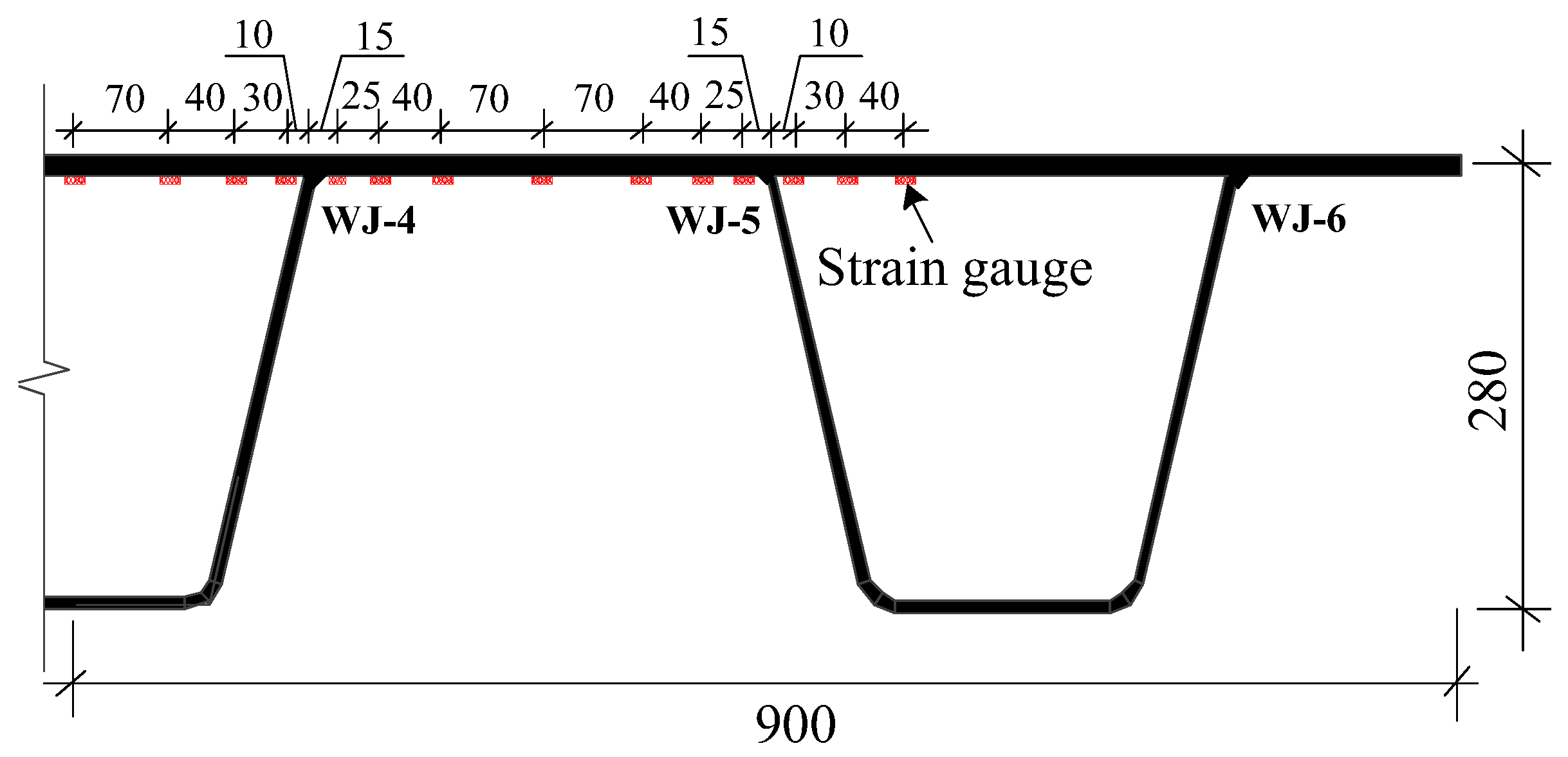
Figure 9 presents the static-load experimental device [37]. The loading force generated by the jack was equally distributed by the distribution beam on the deck plate of the specimen. Therefore, the bending moment of the specimen was consistent between two loading points. The resistance-type strain gauges with the length of 10 mm and the width of 2 mm were adopted as strain-measurement sensors. Due to the symmetry of the structural geometry shape and load, Figure 10 shows the strain gauges distribution of half of the specimen. In this figure, the uniaxial strain gauge was adopted with sensitive grid size of 10 mm $\times$ 3 mm, a resistance value of 120 Ω and a sensitivity coefficient of 2.06. Fourteen strain gauges were distributed on the bottom of the deck, as shown in Figure 10.

Figure 11 shows a comparison between the numerical simulation results and experiment results of the 3U deck-rib component. The experimental study of the deck-rib welding details was undertaken by Ding et al. [37], as shown in Figure 9 and Figure 10. The geometric dimensions, boundary conditions and loading forces of FEM were the same with that of the experiment, as shown in Figure 4. The deck and rib thickness were 16 mm and 8 mm, respectively. The simple support constraints were applied to the left and right ends of the model, and the static-load concentrated force F was 18 KN. In Figure 11, the path of the deck near the weld side at the cross-section Z = 150 mm was selected. The horizontal coordinate X is shown in Figure 4, and the vertical coordinate is the transverse stress $S_x$. In the figure, the curve and the dots represent the numerical simulation results and the experimental results, respectively. The experimental results are the transverse stresses measured by the strain gauges in Figure 10. Figure 11 shows that the maximum value of the numerical simulation results is approximately 294 MPa at the weld toe. The second largest value is approximately 254 MPa at the weld root. The minimum value is approximately 54 MPa. This value was obtained between the weld toe and root (6 mm from the weld root). The experimental results are in good agreement with the numerical simulation results, except for the stress at the weld toe and root. Since the stresses at the weld toe and root cannot be measured in this experiment, the numerical simulation results are considered reliable.

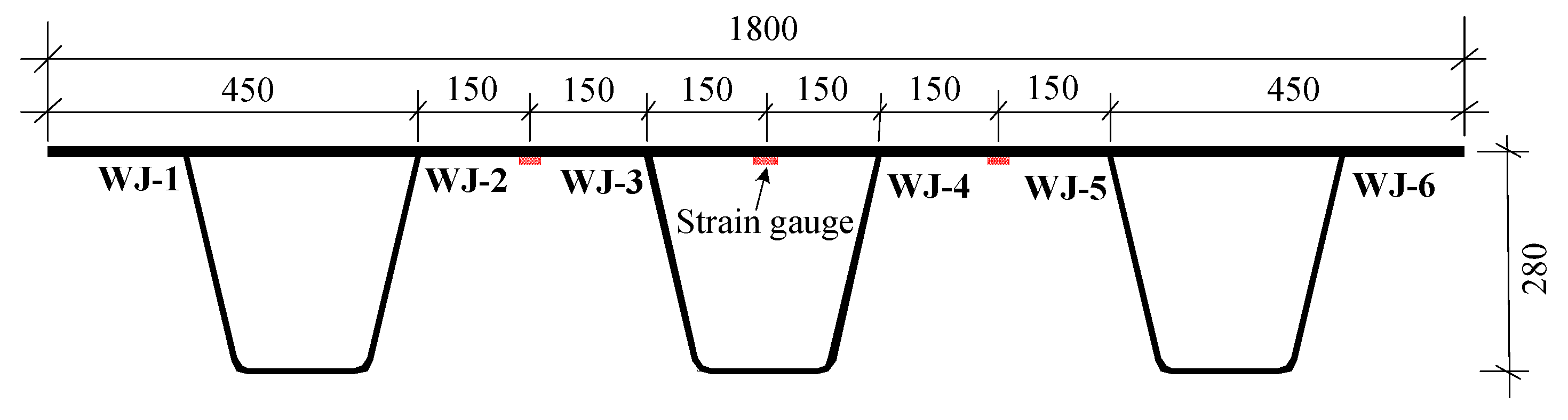
Figure 12 presents the strain gauges distribution in the fatigue experiments [36]. The strain gauges are used to measure nominal stress and located in the middle of two adjacent weld seams, as show in Figure 12.

Table 2. Fatigue experiment results and stress parameters of the 3U component.

Number	Deck Thickness (mm)	Fatigue Crack Location	Fatigue Life (104)	Nominal Stress Range (MPa)	Equivalent Structural Stress Range (MPa)
OSD1	14	WJ-5	27.8	200	232.05
OSD2		WJ-2	93.4	150	270.49
OSD3		WJ-3	43.7	175	308.73
OSD5	16	WJ-5	23.4	200	235.59
OSD6		WJ-2	151.5	150	274.32
OSD7		WJ-5	127.0	175	314.04
OSD9	18	WJ-5	35.2	200	241.17
OSD10		WJ-5	136.7	150	280.34
OSD11		WJ-5	81.6	175	321.68

shows the experiment results of the 3U deck-rib component [37]. The fatigue cracks were all located at the weld toes, and most of them were on the welds of WJ-2 and WJ-5, which are symmetrical positions. In this table, the fatigue life and nominal stress values were obtained from the fatigue experiments [37]. The equivalent stress range $\Delta S_s$ at the weld toe, which has been calculated by Equation (8), was obtained from the corresponding FEM shown in Figure 4.

Figure 13 shows the experimental verification of the master S-N curve for the OSD based on the stress integration approach. The equation of the master S-N curve is shown in Equation (10). In Figure 13, the vertical coordinate is the equivalent structural stress range $\Delta S_s$, and the dots are the experiment data of the equivalent structural stress range in Table 1. Figure 13 shows that the experimental data points are around the mean S-N curve, and all the experiment data points are within the 95% survival rate master S-N curves. Therefore, the master S-N curve with the lower 95% survival rate can be used for the fatigue evaluation of the deck-rib welding details in the OSD under a non-high cycle ($N\le {10}^7$), as shown in Equation (10), where $C_s=13875.8,h=-0.32$.

5. Fatigue Life Calculation of Jiangyin Bridge Based on the Stress Integration Approach

5.1. Multi-Scale Model of Jiangyin Bridge

Jiangyin Yangtze Bridge is located in the Yangtze River delta region, an area with the busiest traffic in China. Fatigue cracks appeared only nine years after the bridge was built [19]. Therefore, it was necessary to adopt an appropriate approach to evaluate the fatigue life of Jiangyin Bridge. Figure 14 shows a multi-scale shell-solid model of Jiangyin Bridge, in which the shell elements and solid elements are used for the full bridge and the local 3U deck-rib weld component, respectively. Command TARGE170 and CONTA175 in Ansys are used for solid185 and shell63, respectively, and rigid connections between them are created, as shown in Figure 14. WJ-R in Figure 14 is the mesh-refined weld joint, which is used to extract stress. The bridge is hinged at both ends along its length direction. The deck thickness and rib thickness of this bridge are 12 mm and 6 mm, respectively.

5.2. Fatigue Vehicle Load

The fatigue standard vehicle load model is shown in Figure 15 [38]. Figure 15a,c show the longitudinal and cross sections of the vehicle, respectively. Figure 15b shows the tire print of the vehicle when moving on the bridge. In Figure 15, the weight of axle 1, axle 2, axle 3 and axle 4 are 50 KN, 100 KN, 90 KN and 90 KN, respectively. Axle 1 was a single wheel, and axle 2, 3, and 4 were double wheels. To consider the dynamic amplification of vehicle load effects, the dynamic amplification coefficient was set as 1.15 [38].

Figure 16 shows the moving vehicle in FEM. Figure 16a shows the longitudinal distribution of the moving vehicle. The length of the vehicle and the segmental bridge are 11.8 m and 18.75 m, respectively. The vehicle moved from the left end of the segmental bridge to the right end at a speed of 16.67 m/s. The simulation of the moving vehicle load in FEM is realized by the cyclic loading method. The load in the the previous step must be deleted before the load in the current step is applied. For each load step, the vehicle moves 0.15 m along the bridge longitudinal direction. Figure 16b shows the transverse distribution of the vehicle load. Uniform pressure was applied on the deck within the vehicle tire print. The resultant force of the wheel pressure was half of the axle weight. In Figure 16b, the resultant force application point of the left wheel is located at WJ-R.

5.3. Stress Time–History Curve

Figure 17 shows the equivalent structural stress and extrapolated hot spot stress time-history curves under the load distribution in Figure 16. The equivalent structural stress analysis point is located at the weld toe of WJ-R, as shown in Figure 17. When the wheel moved above the analysis point, the stress reached the extreme value. The calculation process of equivalent structural stress at four extreme points is given in

Table 3. Calculation of equivalent structural stress.

Time (s)	${\mathit{\sigma }}_{\mathit{m}}\left(\mathbf{MPa}\right)$	${\mathit{\sigma }}_{\mathit{b}}\left(\mathbf{MPa}\right)$	$\mathit{r}$	$\mathit{I}{\left(\mathit{r}\right)}^{\frac{1}{\mathit{n}}}$	${\mathit{t}}^{\ast }$	${\mathit{\sigma }}_{\mathit{s}}\left(\mathbf{MPa}\right)$	${\mathit{S}}_{\mathit{s}}\left(\mathbf{MPa}\right)$
0.56	−0.49	−20.39	0.98	1.32	12	−20.88	−27.39
0.77	−1.05	−44.73	0.98	1.32	12	−45.78	−60.03
1.19	−0.94	−40.25	0.98	1.32	12	−41.19	−54.02
1.27	−0.95	−40.79	0.98	1.32	12	−41.74	−54.74

. In this table, the bending stress ${\sigma }_b$ is much larger than the membrane stress ${\sigma }_m$, which is the main stress causing the crack at the weld toe. The bending ratio $r$, which is defined as the absolute value of the ratio of bending stress to the sum of bending stress and membrane stress, is almost the same at different times. As a comparison, the stress time history curve of extrapolating the hot spot stress is also given in Figure 17. To calculate the hot spot stress, the mesh size was 1 mm, refined at the weld seam. The transverse stresses at 0.4t and 1.0t can be extracted and substituted into Equation (11) to obtain the extrapolated hot spot stress. In Figure 17, the maximum absolute value of the extrapolated hot spot stress is approximately 45 MPa, which is only 75% that of the equivalent structural stress.

5.4. Fatigue Life Calculation of Jiangyin Bridge Based on the Stress Integration Approach

In order to be consistent with the form in the codes, Equation (10) is rewritten as Equation (13):

$$\Delta S_s{}^m\cdot N=C$$

(13)

where $\Delta S_s$ is the equivalent structural stress range, $m=-1/h=3.125,$ $C={13875.8}^m=8.801\times {10}^{12}$.

The slope m of the master S-N curve in Equation (13) given by Dong et al. was 3.125. This is close to the slope m = 3 of the S-N curves in the codes [9,12] under the low cycles. However, in these codes [9,12], the slope of the S-N curve changes under high cycles. Most experimental data points beyond the 99% survival rate are under high cycles ($N>{10}^7$), as shown in Figure 4 of the reference [13]. Therefore, it is not suitable that the master S-N curve adopts a single slope m = 3.125 from low to high cycles. Referring to the S-N curve of the hot spot stress approach in IIW [12], the slope of the master S-N curve is set as 5 under high cycles ($N>{10}^7$), as shown in Equation (14).

$$\{\begin{array}{l}\Delta S_s{}^{m_1}\cdot N=8.801\times {10}^{12}\left(m_1=3.125,N\le {10}^7\right)\\ \Delta S_s{}^{m_2}\cdot N=3.246\times {10}^{16}\left(m_2=5,N>{10}^7\right)\end{array}$$

(14)

The calculation formula of the hot spot stress approach is also given as a comparison, as shown in Equation (15).

$$\{\begin{array}{l}\Delta {\sigma }_{hs}{}^{m_1}\cdot N=2\times {10}^{12}\left(m_1=3,N\le {10}^7\right)\\ \Delta {\sigma }_{hs}{}^{m_2}\cdot N=6.851\times {10}^{15}\left(m_2=5,N>{10}^7\right)\end{array}$$

(15)

The fatigue life calculation steps based on the stress integration approach:

(1) The principal stress ${\sigma }_x\left(y,z\right)$ of the weld toe section is extracted from FEM. Then, the structural stress value ${\sigma }_s$ is obtained by substituting ${\sigma }_x\left(y,z\right)$ into Equation (7). Then, the equivalent structural stress $S_s$ is obtained by substituting ${\sigma }_s$ into Equation (10). The equivalent structural stress time-history curve can be obtained in this step, as shown in Figure 14.

(2) The equivalent stress range $\Delta S_{seq}$ and stress cycle times $n_{eq}$ are calculated by the rain-flow counting method.

(3) The equivalent stress range $\Delta S_{seq}$ is substituted into the master S-N curve using Equation (13) or Equation (14) to obtain the number of cycles $N$.

(4) Damage $D_j$ under a load case j is calculated, as shown in Equation (16). According to the structural health monitoring results, daily traffic volume $N_{v,d}$ equals to 2551 [19] and wheel transverse distribution frequency $f_j$ is shown in Figure 15 of the reference [39].

$$D_j=\frac{365\cdot f_j\cdot n_{eq,j}\cdot N_{v,d}}{N_j}$$

(16)

(5) The fatigue life $N_a$ is calculated by Equation (17), where $D_T$ is the total damage.

$$N_a=\frac{1}{D_T}=\frac{1}{{\displaystyle \sum D_j}}$$

(17)

Taking the load case in Figure 16 as an example, the fatigue life calculation steps based on the stress integration approach are shown in

Table 4. Fatigue life calculation steps.

Approach	Equation No.	Step
		(1)	(2)		(3)	(4)	(5)
		Stress Time History Curve	$\mathbf{\Delta }{\mathit{S}}_{\mathit{e}\mathit{q}}\left(\mathbf{MPa}\right)$	${\mathit{n}}_{\mathit{e}\mathit{q}}$	$\mathit{N}$$(\times {10}^7)$	${\mathit{D}}_4$	${\mathit{D}}_{\mathit{T}}$	${\mathit{N}}_{\mathit{a}}\left(\mathbf{years}\right)$
Extrapolated hot spot stress	$\mathrm{Equation}\left(15\right)m_1=3,m_2=5$	Figure 17	40.25	4	6.4852	0.0099	0.0121	83
Stress integration	$\mathrm{Equation}\left(13\right)m_1=3.125,m_2=5$	Figure 17	54.89	4	6.5136	0.0098	0.0119	84
	$\mathrm{Equation}\left(14\right)m_1=m_2=3.125$	Figure 17	54.89	4	3.2258	0.0194	0.0303	33

. As a comparison, the results of the extrapolated hot spot stress approach are also given, and the extrapolated hot spot stress time-history curve and Equation (15) should be used in step (1) and (3), respectively, in this case. In Table 4, $m_1$ and $m_2$ are the slope of the S-N curve at non-high cycles $N\le {10}^7$ and high cycles $N>{10}^7$, respectively. The fatigue life calculated by the stress integration approach is 84 years under the slope $m_2=5$ and 33 years under the slope $m_2=3.125$, respectively, and the fatigue life of the former is 2.5 times that of the latter. Therefore, the slope of the master S-N curve at high cycles significantly affects the actual bridge fatigue life. The fatigue life calculated by the stress integration approach and the extrapolated hot spot stress approach are very similar, at 84 and 83 years respectively. Therefore, the slope $m_2=5$ of the master S-N curve at high cycles is more reasonable.

The total damage $D_T$ in Table 4 is the sum of the damage under six main load cases, as shown in Figure 18. A distance of 0.15 m along the transverse direction was assumed as a case of distribution. The wheel load transverse distribution frequencies are shown in Figure 15 of the reference [39]. For simplicity, Figure 18 only shows the load distribution of double wheels. The details of the load distribution under case 4 in Figure 18 refers to Figure 16. The damage $D_j$ calculated by the stress integration approach with $m_2=5$ under six different load cases is given in Figure 18. This shows that the maximum damage occurs under load case 4, followed by case 3 and case 5, and the damage is small under other cases. The damage value under load case 4 is approximately 80% of the total damage.

6. Influence of Weld Parameters on the Fatigue Life of Deck-Rib Welding Details in the OSD

6.1. Influence of Weld Size on the Bridge Fatigue Life

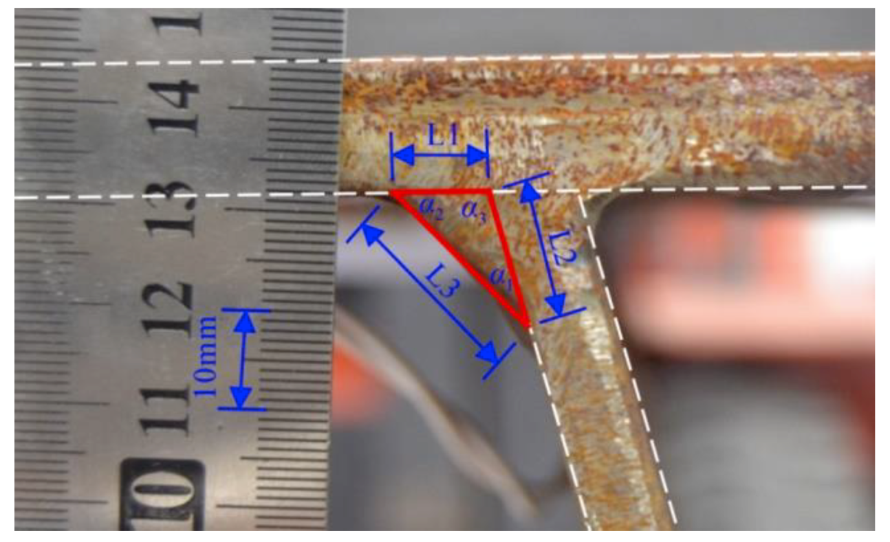
Figure 19 shows the measurement of deck-rib weld sizes in the experiment. In Figure 19, $L_1,L_2$ and $L_3$ are the three sides of the weld triangle. The measured weld sizes are listed in

Table 5. Measured weld size of the experiment components (unit: mm).

Weld no.	L1	L2	L3	Weld no.	L1	L2	L3
1	10.9	11.4	17.5	20	5.4	7.1	10.0
2	7.4	12.2	15.8	21	10.7	7.8	14.3
3	9.6	12.0	16.8	22	9.9	6.3	12.9
4	8.7	10.4	15.0	23	10.2	9.5	15.1
5	8.6	9.4	13.9	24	8.4	7.9	12.6
6	8.7	16.2	20.0	25	6.9	9.3	12.4
7	9.5	10.5	15.4	26	12.4	12.1	18.9
8	10.4	10.5	16.0	27	10.4	10.9	16.3
9	8.9	11.7	15.9	28	8.2	13.6	17.6
10	10.6	9.8	15.9	29	9.8	10.7	15.6
11	11.6	12.4	18.8	30	9.8	8.8	14.5
12	12.7	11.8	19.2	31	9.7	11.0	15.9
13	11.6	12.4	18.7	32	8.9	9.8	14.2
14	10.3	11.2	16.7	33	11.0	11.8	17.5
15	7.2	8.7	12.5	34	10.4	15.0	19.8
16	8.8	7.6	12.8	35	10.9	11.1	17.0
17	7.9	12.1	15.9	36	10.7	10.8	16.4
18	10.0	7.8	13.8	37	10.8	10.7	15.8
19	9.4	7.1	13.0	38	10.5	9.6	15.6

.

${\alpha }_1,{\alpha }_2$ and ${\alpha }_3$ are the three angles calculated by $L_1,L_2$ and $L_3$, as shown in Figure 16. The mean, minimum and maximum values of the weld size are shown in

Table 6. Mean, minimum and maximum values of the weld size.

Statistics Value	${\mathit{L}}_1\left(\mathbf{mm}\right)$	${\mathit{L}}_2\left(\mathbf{mm}\right)$	${\mathit{L}}_3\left(\mathbf{mm}\right)$	${\mathit{\alpha }}_1(°)$	${\mathit{\alpha }}_2(°)$	${\mathit{\alpha }}_3(°)$
Mean	9.68	10.5	15.68	37.14	40.92	101.94
Minimum	5.4	6.3	10	25.11	28.38	94.59
Maximum	12.7	16.2	20	48.32	52.21	105.45

.

Since the measured actual weld size is discrete, which is mainly caused by weld manufacturing errors, five representative weld types (WTs) were selected in the present study, as shown in Figure 20 and

Table 7. Size of five weld types (unit: mm).

Weld Types	${\mathit{\alpha }}_1$	${\mathit{\alpha }}_2$	${\mathit{\alpha }}_3$	L1	L2	L3	Area
WT-1	30	50	100	5.2	8	10.28	20.57
WT-2	40	40	100	8	8	12.26	31.51
WT-3	50	30	100	12.3	8	15.76	48.28
WT-4	40	40	100	10	10	15.32	49.24
WT-5	40	40	100	12.5	12.5	19.15	76.94

. In Table 7: (1) The angle ${\alpha }_3$ remains at 100 degrees. The size of weld type 4 (WT-4) is close to the mean value in Table 6. The length $L_1$ of WT-1 and WT-5 are close to the minimum value and maximum value in Table 6, respectively, and the rest of the values are within the extreme range. (2) A comparison of WT-1, WT-2 and WT-3 shows that the length $L_1$ increases successively when the length $L_2$ remains unchanged. That is, the angle ${\alpha }_2$ between the deck and rib decreases by 10 degrees successively. (3) A comparison of WT-2, WT-4 and WT-5 shows that the weld angles remain the same, and the length of three sides increases by an equal proportion of 25% successively. That is, the weld area increases by 56% successively. (4) The length $L_1$ of WT-5 is approximately equal to that of WT-3, and the length of $L_2$ is extended by 56%.

Figure 21 shows the variation of fatigue life with the weld size under the standard vehicle load in Figure 15. In Figure 21, $m_2$ is the slope of the master S-N curve at high cycles $N>{10}^7$ using the stress integration approach. The fatigue life calculation steps are shown in Section 5.4, and the fatigue life of WT-4 is shown in Table 4.

Figure 21 shows the following:

(1) The fatigue life of the stress integration approach with slope $m_2=5$ is close to that of the extrapolated hot spot stress approach. However, the fatigue life with slope $m_2=3.125$ is less than half that of the extrapolated hot spot stress approach. Therefore, the slope of the master S-N curve at high cycles significantly affects the bridge fatigue life, and the slope $m_2=5$ is more reasonable.

(2) The fatigue lives of WT-1, WT-2, WT-3, WT-4 and WT-5 are approximately 51 years, 69 years, 113 years, 84 years and 100 years, respectively, and only reach approximately 100 years under a standard vehicle load. Thus, the change of the weld size can obviously affect the bridge fatigue life. The fatigue life of the most favorable condition, WT-3, is 2.2 times that of the most unfavorable, WT-1.

(3) The comparison of WT-1, WT-2 and WT-3 shows that the fatigue life increases obviously with the decrease of the angle ${\alpha }_2$ between the weld and the deck. The fatigue life increases by approximately 50% with the decrease of angle ${\alpha }_2$ by 10 degrees.

(4) The comparison of WT-2, WT-4 and WT-5 shows that when the weld angles remain the same, the fatigue life increases with the increase of the weld area. The fatigue life increases by approximately 20% with the weld area increasing by 56% (or the length of three sides increasing by 25% with the same proportions).

(5) The comparison of WT-3 and WT-5 shows that the fatigue life decreases with the increase of $L_2$, when the length of $L_1$ is approximately equal. The fatigue life decreases by approximately 12% with the increase of $L_2$, by 56%. Although the weld area increases in this case, the fatigue life decreases due to the increased angle ${\alpha }_2$ between the deck and the weld.

(6) Therefore, the change of weld size caused by weld manufacturing errors can obviously affect the actual bridge fatigue life. The fatigue life of five different weld types varies from 51 years to 113 years under a standard vehicle load. The weld fatigue life increases with the decrease of the angle ${\alpha }_2$ between the deck and the rib and the increase of the weld area. The most favorable weld type is WT-3, with the angle ${\alpha }_2$ of 30 degrees and the area of 48 mm².

6.2. Grinding Treatment

It can be seen from the results in the previous section that the decrease of the angle between the deck and the weld can significantly improve the fatigue life of the deck-rib welding details. The reason is that the stress concentration at the weld toe decreases with the decrease of the angle between the weld and the deck. For the same reason, grinding treatment can also reduce the stress concentration at the weld by smoothing the transition between the deck and the weld.

6.2.1. Influence of Grinding Types

The two grinding types and their FEMs are shown in Figure 22. In Figure 22, the parameters $r$, $d$ and $\phi$ are the grinding radius, grinding depth, and the angle between the axial direction of the grinder head and the deck, respectively. These parameters for two grinding types are shown in

Table 8. The effects of different grinding types on fatigue life.

Grinding Type	$\mathit{r}$ (mm)	$\mathit{d}$ (mm)	$\mathit{\phi }$$(\circ )$	${\mathit{S}}_{\mathit{s}}\left(\mathbf{MPa}\right)$	${\mathit{N}}_{\mathit{a}}\left(\mathbf{years}\right)$
Non-grinding	—	—	—	55.35	84
GT1	3	0.5	70	58.53	63
GT2	3	0	50	54.31	92

. The grinding radius r and depth of grinding type 1 (GT1) are 3 mm and 0.5 mm, respectively, and the grinding arc intersects with the deck [34]. The grinding type 2 (GT2) is a new grinding type proposed in the present study. The grinding radius $r$ is also 3 mm and the grinding depth $d$ is 0. that is, the grinding arc is tangent to the deck without weakening the deck. In the grinding treatment process, the main difference between GT2 and GT1 is the angle $\phi$ between the axial direction of the grinder head and the deck. Nonetheless, how to accurately control the angle is a key issue to be considered in the experiment design. A comparison of different grinding types is shown in Table 8.

Table 8 shows the comparison of different grinding types. For GT1, the equivalent structural stress $S_s$ increases by 5.75% and the fatigue life $N_a$ decreases by 25% compared with the non-grinding type. For GT2, the equivalent structural stress $S_s$ decreases by 1.88% and the fatigue life $N_a$ increases by 10% compared with the non-grinding type. Since GT2 can reduce the stress concentration at the weld toe without weakening the deck section, it is more conducive to improving the fatigue life of the weld.

6.2.2. Influence of Grinding Radius

Figure 23 shows the finite element models with different grinding radii of GT2 under WT-4. In Figure 23, 12 mm is the maximum grinding radius to ensure that both the deck and the rib are not weakened. For WT-1, WT-2, WT-3, WT-4 and WT-5, the maximum grinding radius is 6 mm, 8 mm, 14 mm, 12 mm and 14 mm, respectively. After the grinding treatment, all the welds meet the requirements in the code that the height of the weld throat is not less than the thickness of the rib [38].

According to the fatigue life calculation steps in Section 5.4, the variation of the fatigue life with the grinding radius for GT2 under different weld types is shown in Figure 24. In this figure:

(1) A comparison of WT-1, WT-2 and WT-3 shows that when the grinding radius changes from 0 to 2 mm, the fatigue life of WT-1, WT-2 and WT-3 increases by 14%, 5% and −1.5%, respectively. This indicates that the grinding treatment has an obvious effect on increasing fatigue life when the angle ${\alpha }_2$ between the deck and the weld is large.

(2) When the grinding radius is greater than 2 mm, the curves of the fatigue life as they vary with the grinding radius under different weld types are almost parallel, which indicates that when the grinding radius is large, the influence of the grinding radius on the fatigue life has little relation to the weld type.

(3) For different weld types, when the grinding radius is greater than 2 mm, the fatigue life at the weld toe increases with the increase of the grinding radius. The fatigue life increases by approximately 5% when the grinding radius increases by 2 mm.

(4) A larger grinding radius is conducive to improving the bridge fatigue life, but at the same time, it can increase the weakening of the weld seam itself, which may lead to cracks in the weld throat. Therefore, further experimental research is needed to select an appropriate grinding radius which both ensures fatigue cracks do not appear in the weld throat and maximizes the fatigue life at the weld toe.

6.3. Influence of the Weld Penetration Rate

The penetration rate of the deck-rib welding details shall not be lower than 80% in the code [8]. To study the influence of the weld penetration rate on the bridge fatigue life, a FEM of 80% partial penetration and 100% full penetration for WT-4 are shown in Figure 25. According to the fatigue life calculation steps in Section 5.4, the structural stress and fatigue life of 80% partial penetration and 100% full penetration at the weld toe were calculated, as shown in

Table 9. Comparison of structural stress and fatigue life under different penetration rates.

Penetration Rate	${\mathit{\sigma }}_{\mathit{s}}\left(\mathbf{MPa}\right)$	${\mathit{S}}_{\mathit{s}}\left(\mathbf{MPa}\right)$	${\mathit{N}}_{\mathit{a}}\left(\mathbf{Years}\right)$
80%	41.67	54.64	89
100%	42.21	55.35	84

. Compared with 100% full penetration, the structural stress ${\sigma }_s$ and equivalent structural stress $S_s$ of the weld toe under 80% partial penetration were reduced by approximately 1.3%, and the fatigue life $N_a$ increased by approximately 5.6%. Therefore, the fatigue life of 80% partial penetration is slightly higher than that of 100% full penetration.

7. Conclusions

• The stress integration approach for the 3D solid elements showed that the structural stress does not change significantly with the parameters $w$ (width of the isolated body) and $\delta$ (the distance between the crack propagation surface and the reference surface). In order to simplify the calculation, $\delta$ was set as 0, and $w$ can be set as the mesh size along the weld length direction.
• When the mesh size is no more than 0.5 times the deck thickness, the mesh insensitivity of the stress integration approach is obviously better than that of the extrapolation hot spot stress approach. The mesh size in the stress integration approach is recommended to be 0.25 times the deck thickness, and the calculation error is approximately 2%.
• The slope of the master S-N curve at high cycles ($N>{10}^7$) significantly affects the bridge fatigue life, and the slope $m_2=5$ at high cycles is more reasonable.
• The weld parameter analysis for Jiangyin Bridge showed the following: (1) The change of weld size caused by weld manufacturing errors can obviously affect the bridge fatigue life. The fatigue life of five different weld types varies from 51 years to 113 years under a standard vehicle load. The weld fatigue life increases with the decrease of the angle ${\alpha }_2$ between the deck and the rib and the increase of the weld area. (2) A new grinding treatment type that does not weaken the deck is proposed. It is more beneficial to improve the fatigue life of the deck-rib welding details, and the fatigue life increases by approximately 5% when the grinding radius increases by 2 mm. (3) The fatigue life with 80% partial penetration is slightly higher than that of 100% full penetration. (4) In practice, the most favorable weld type is WT-3 with an angle ${\alpha }_2$ of 30 degrees and an area of 48 mm². The grinding type that does not weaken the deck is more conducive to improving the bridge fatigue life. The 80% partial penetration of the deck-rib welding details condition is recommended.

References

1. Xiao, Z.G.; Yamada, K.; Ya, S.; Zhao, X.L. Stress analyses and fatigue evaluation of rib-to-deck joints in steel orthotropic decks. Int. J. Fatigue 2008, 30, 1387–1397. [Google Scholar] [CrossRef]
2. Ya, S.; Yamada, K.; Ishikawa, T. Fatigue evaluation of rib-to-deck welded joints of orthotropic steel bridge deck. J. Bridge Eng. 2011, 492–499. [Google Scholar] [CrossRef]
3. Fisher, J.; Barsom, J. Evaluation of cracking in the rib-to-deck welds of the Bronx–Whitestone Bridge. J. Bridge Eng. 2016. [Google Scholar] [CrossRef]
4. De Jong, F. Renovation Techniques for Fatigue Cracked Orthotropic Steel Bridge Decks. Ph.D. Thesis, Delft University of Technology, Delft, The Netherlands, 2006. [Google Scholar]
5. Cui, C.; Bu, Y.Z.; Zhang, Q.H.; Li, L.J. Fatigue Life Assessment of Orthotropic Steel Deck Plate Based on Hot Spot Stress Method. Bridge Constr. 2014, 44, 62–65. [Google Scholar]
6. Liu, R.; Liu, Y.; Ji, B.; Wang, M.; Tian, Y. Hot spot stress analysis on rib-deck welded joint in orthotropic steel decks. J. Constr. Steel Res. 2014, 97, 1–9. [Google Scholar]
7. Zhang, Q.H.; Cui, C.; Bu, Y.Z.; Liu, Y.M.; Ye, H.W. Fatigue tests and fatigue assessment approaches for rib-to-diaphragm in steel orthotropic decks. J. Constr. Steel Res. 2015, 114, 110–118. [Google Scholar] [CrossRef]
8. American Association of State Highway and Transportation Officials (AASHTO). Guide Specifications for Fatigue Evaluation of Existing Steel Bridges; AASHTO: Washington, DC, USA, 2004. [Google Scholar]
9. CEN (European Committee for Standardization). Design of Steel Structures, Part 1–9: Fatigue. Eurocode3; CEN: Brussels, Belgium, 1992. [Google Scholar]
10. Sun, Y.; Yang, X. Study on the Correction of S-N Distribution in the Welding Fatigue Analysis Method Based on the Battelle Equivalent Structural Stress by Rough Set Theory. J. Mech. Eng. 2014, 60, 600–606. [Google Scholar] [CrossRef]
11. Niemi, E.; Tanskanen, P. Hot spot stress determination for welded edge gussets. Weld. World 2000, 44, 31–37. [Google Scholar]
12. Hobbacher, A. Recommendations for Fatigue Design of Welded Joints and Components; IIW Document XIII-2151r1-07/XV-1254r1-07; International Institute of Welding (IIW): Paris, France, 2007. [Google Scholar]
13. Dong, P.; Prager, M.; Osage, D. The Design Master S-N Curve in ASME Div 2 Rewrite and its Validations. Weld. World 2007, 51, 53–63. [Google Scholar] [CrossRef]
14. Dong, P. A robust structural stress method for fatigue analysis of offshore/marine structures. ASME J. Offshore Mech. Arct. Eng. 2005, 127, 68–74. [Google Scholar] [CrossRef]
15. Kyuba, H.; Dong, P. Equilibrium-equivalent structural stress approach to fatigue analysis of a rectangular hollow section joint. Int. J. Fatigue 2005, 27, 85–94. [Google Scholar] [CrossRef]
16. Feng, B. Hot Spot Stress Analysis of the Construction Details of Highway Orthotropic Deck and Fatigue Research. Master’s Thesis, Southwest Jiaotong University, Chengdu, China, 2011. [Google Scholar]
17. Fang, Z.; Li, A.Q.; Li, W.R.; Shen, S. Wind-Induced Fatigue Analysis of High-Rise Steel Structures Using Equivalent Structural Stress Method. Appl. Sci. 2017, 7, 71. [Google Scholar] [CrossRef]
18. Dong, P.; Pei, X.; Xing, S.; Kim, M.H. A structural strain method for low-cycle fatigue evaluation of welded components. Int. J. Press. Vessel. Pip. 2014, 119, 39–51. [Google Scholar]
19. Cao, B.Y.; Ding, Y.L.; Song, Y.S.; Zhong, W. Fatigue Life Evaluation for Deck-rib Welding Details of Orthotropic Steel Deck Integrating Mean Stress Effects. J. Bridge Eng. 2019, 24, 04018114. [Google Scholar] [CrossRef]
20. Li, J.; Zhang, Q.H.; Bao, Y.; Zhu, J.Z.; Chen, L.; Bu, Y.Z. An equivalent structural stress-based fatigue evaluation framework for rib-to-deck welded joints in orthotropic steel deck. Eng. Struct. 2019, 196, 109304. [Google Scholar] [CrossRef]
21. Wang, P.; Pei, X.; Dong, P.; Song, S. Traction structural stress analysis of fatigue behaviors of rib-to-deck joints in orthotropic bridge deck. Int. J. Fatigue 2019, 125, 11–22. [Google Scholar] [CrossRef]
22. Zhang, Q.H.; Bu, Y.Z.; Li, Q. Review on fatigue problems of orthotropic steel bridge deck. China J. Highw. Transp. 2017, 30, 14–30. [Google Scholar]
23. Luo, P.J.; Zhang, Q.H.; Bao, Y. Predicting weld root notch stress intensity factors for rib-to-deck welded joint under deck loading modes. Int. J. Fatigue 2019, 128, 105212. [Google Scholar] [CrossRef]
24. Luo, P.J.; Zhang, Q.H.; Bao, Y.; Bu, Y.Z. Fatigue performance of welded joint between thickened-edge U-rib and deck in orthotropic steel deck. Eng. Struct. 2019, 181, 699–710. [Google Scholar] [CrossRef]
25. Heng, J.L.; Zheng, K.F.; Chao, G.; Yu, Z.; Yi, B. Fatigue performance of rib-to-deck joints in orthotropic steel decks with thickened edge U-ribs. J. Bridge Eng. 2017, 22, 04017059. [Google Scholar] [CrossRef]
26. Wang, J.B. Research on Hot Spot Stress Approach of Fatigue Evaluation and Application for High Speed Car. Ph.D. Thesis, Beijing Jiaotong University, Beijing, China, 2008. [Google Scholar]
27. Cao, V.D.; Sasaki, E.; Tajima, K.; Suzuki, T. Investigations on the effect of weld penetration on fatigue strength of rib-to-deck welded joints in orthotropic steel decks. Int. J. Steel Struct. 2015, 15, 299–310. [Google Scholar]
28. Liu, X.Y. Study on the Welding Residual Stress in Anchorage Area of Steel Bridge. Adv. Mater. Res. 2011, 255, 324–327. [Google Scholar]
29. Shimanuki, H.; Okawa, T. Effect of stress ratio on the enhancement of fatigue strength in high performance steel welded joints by ultrasonic impact treatment. Int. J. Steel Struct. 2013, 13, 155–161. [Google Scholar]
30. Cui, C.; Qinghua, Z.; Yi, B.; Jiping, K.; Yizhi, B. Fatigue performance and evaluation of welded joints in steel truss bridges. J. Constr. Steel Res. 2018, 148, 450–456. [Google Scholar] [CrossRef]
31. Fu, Z.Q.; Ji, B.H.; Xie, S.H.; Liu, T.J. Crack stop holes in steel bridge decks: Drilling method and effects. J. Cent. South Univ. 2017, 24, 2372–2381. [Google Scholar]
32. Xie, F.X.; Ji, B.H.; Yuanzhou, Z.Y.; Fu, Z.Q.; Ge, H.B. Ultrasonic detecting method and repair technology based on fatigue crack features in steel box girder. J. Perform. Constr. Facil. 2016, 30, 04015006. [Google Scholar] [CrossRef]
33. Fu, Z.; Wang, Q.; Ji, B.; Yuanzhou, Z. Rewelding Repair Effects on Fatigue Cracks in Steel Bridge Deck Welds. J. Perform. Constr. Facil. 2017, 31, 04017094. [Google Scholar]
34. Fu, Z.; Ji, B.; Kong, X.; Chen, X. Grinding treatment effect on rib-to-roof weld fatigue performance of steel bridge decks. J. Constr. Steel Res. 2017, 129, 163–170. [Google Scholar]
35. Sim, H.B.; Uang, C.M. Stress Analyses and Parametric Study on Full-Scale Fatigue Tests of Rib-to-Deck Welded Joints in Steel Orthotropic Decks. J. Bridge Eng. 2012, 17, 765–773. [Google Scholar] [CrossRef]
36. Fu, Z.; Ji, B.; Zhang, C.; Wang, Q. Fatigue Performance of Roof and U-Rib Weld of Orthotropic Steel Bridge Deck with Different Penetration Rates. J. Bridge Eng. 2017, 22, 04017016. [Google Scholar]
37. Ding, Y.L.; Song, Y.S.; Cao, B.Y.; Wang, G.X.; Li, A.Q. Full-Range S-N Fatigue-Life Evaluation Method for Welded Bridge Structures Considering Hot-Spot and Welding Residual Stress. J. Bridge Eng. 2016, 21, 04016096. [Google Scholar] [CrossRef]
38. Industry Standard of the People’s Republic of China. Guidelines for Design and Maintain of Orthotropic Steel Deck; China Architecture & Building Press: Beijing, China, 2010. [Google Scholar]
39. Fu, Z.; Ji, B.; Ye, Z.; Wang, Y. Fatigue evaluation of cable-stayed bridge steel deck based on predicted traffic flow growth. KSCE J. Civ. Eng. 2017, 21, 1–10. [Google Scholar]
Figure 1. Fatigue cracks in the Jiangyin Yangtze River Bridge.
Applsci 09 03917 g001
Figure 2. Stress distribution and decomposition at the weld toe section.
Applsci 09 03917 g002
Figure 3. Stress distribution of the 3D solid element isolated body.
Applsci 09 03917 g003
Figure 4. The multi-scale finite element model (FEM) of the deck-rib component (units: mm).
Applsci 09 03917 g004
Figure 5. Variation of structural stress with the parameters δ and w . (a) The parameter δ ( w = 2 mm). (b) The parameter w ( δ = 0 ).
Applsci 09 03917 g005
Figure 6. Mesh sizes of deck-rib welding details.
Applsci 09 03917 g006
Figure 7. Variation of structural stress with mesh size.
Applsci 09 03917 g007
Figure 8. Error comparison of different approaches.
Applsci 09 03917 g008
Figure 9. Static-load experimental device.
Applsci 09 03917 g009
Figure 10. Strain gauges distribution (units: mm).
Applsci 09 03917 g010
Figure 11. Comparison of the numerical simulation results with the experiment results.
Applsci 09 03917 g011
Figure 12. Strain gauges distribution in the fatigue experiments (units: mm).
Applsci 09 03917 g012
Figure 13. Experiment verification of the master S-N curve for the orthotropic steel decks (OSD).
Applsci 09 03917 g013
Figure 14. Multi-scale model of the Jiangyin Bridge.
Applsci 09 03917 g014
Figure 15. Fatigue load model.
Applsci 09 03917 g015
Figure 16. Moving vehicle in the FEM. (a) Moving vehicle longitudinal distribution; (b) Vehicle transverse distribution.
Applsci 09 03917 g016
Figure 17. Stress time-history curve.
Applsci 09 03917 g017
Figure 18. Damage under six load cases.
Applsci 09 03917 g018
Figure 19. Weld dimension measurement.
Applsci 09 03917 g019
Figure 20. Weld types.
Applsci 09 03917 g020
Figure 21. Variation of fatigue life with weld size.
Applsci 09 03917 g021
Figure 22. Grinding type. (a) Grinding type 1. (b) Grinding type 2.
Applsci 09 03917 g022
Figure 23. Finite element models of different grinding radii.
Applsci 09 03917 g023
Figure 24. Variation of fatigue life with grinding radius.
Applsci 09 03917 g024
Figure 25. FEM of 80% partial penetration and 100% full penetration. (a) 80% (b) 100%.
Applsci 09 03917 g025