Feature Extraction of Impulse Faults for Vibration Signals Based on Sparse Non-Negative Tensor Factorization

Featured Application

The proposed feature extraction method can be typically applied in the fault diagnosis of rolling bearings and other rotating machinery.

Abstract

The incipient damages of mechanical equipment excite weak impulse vibration, which is hidden, almost unobservable, in the collected signal, making fault detection and failure prevention at the inchoate stage rather challenging. Traditional feature extraction techniques, such as bandpass filtering and time-frequency analysis, are suitable for matrix processing but challenged by the higher-order data. To tackle these problems, a novel method of impulse feature extraction for vibration signals, based on sparse non-negative tensor factorization is presented in this paper. Primarily, the phase space reconstruction and the short time Fourier transform are successively employed to convert the original signal into time-frequency distributions, which are further arranged into a three-way tensor to obtain a time-frequency multi-aspect array. The tensor is decomposed by sparse non-negative tensor factorization via hierarchical alternating least squares algorithm, after which the latent components are reconstructed from the factors by the inverse short time Fourier transform and eventually help extract the impulse feature through envelope analysis. For performance verification, the experimental analysis on the bearing datasets and the swashplate piston pump has confirmed the effectiveness of the proposed method. Comparisons to the traditional methods, including maximum correlated kurtosis deconvolution, singular value decomposition, and maximum spectrum kurtosis, also suggest its better performance of feature extraction.

1. Introduction

In modern industry, the increasing complexity of mechanical equipment assigns great significance to the normal operation of every single part. An unexpected failure could lead to the instability or even breakdown of the mechanical system [1,2]. In engineering practice, incipient fault prognosis is expected to provide early warning before the occurrence of catastrophic failure.

Evidently, vibration signals are effective tools for condition monitoring and fault diagnosis, mainly because of their revelations of dynamic information and their convenience for measurements. In Stanisław’s study, various measurement systems for evaluating the vibrations of rolling bearings were thoroughly compared [3]. Generally, due to the complexity of the transmission, the vibration signal with incipient fault often incorporates a large amount of the interference apart from the fault characteristic components. The interference may include the harmonic components that are related to operational status and stochastic noise, such as electromagnetic interference. Thus, the feature of impulse fault is inundated and covered unobservable in the data.

To date, plenty of studies have been carried out to identify the impulse fault components. In the theory of probability and statistics, the kurtosis, as a measure for the shape of data distribution, is conducive to capture the outliers (e.g., abnormal impulses) in the data [4]. Jia et al. further investigated that peculiarity, enforcing the impulses in the signal, in an improved algorithm named the maximum correlated kurtosis deconvolution (MCKD), to indicate the periodic fault transients [5]. MCKD has received growing attention, and it can be categorized as a single-dimensional method.

With respect to two-dimensional methods like time-frequency analysis, the time-frequency distribution (TFD) obtained by short time Fourier transform (STFT) [6], Wigner distribution, wavelet transform [7], etc., provides an effective tool for analyzing non-stationary vibration signals, as it incorporates information from both the time-domain and frequency-domain. Also, it is interesting to note that relevant studies based on matrix analysis emerged. Given the non-negativity of TFD, Lin et al. combined the time-frequency analysis with non-negative matrix factorization for feature extraction in [8]. Leng et al. utilized singular value decomposition (SVD) to identify relevant information from background noise, which was combined with envelope analysis to detect a fault feature of rolling bearings in [9]. Jiang et al. introduced the ratios of neighboring singular values to distinguish different beating fault types [10]. Specifically, SVD resorts to the Hankel matrix to obtain a two-dimensional representation for a time series, which signals the trend of the high-dimension analysis. The study of Qingbo and Xiaoxi reports a combination of time-frequency analysis and manifold learning for signature enhancement [11], in which phase space reconstruction (PSR) is used for constructing a three-dimensional TFD manifold. It provides finesse for enhancing the impulse feature, but inconvenience appears, as the TFDs must be changed into vectors for manifold learning. The techniques mentioned are admittedly efficacious for feature extraction in two-dimensional representations; however, the applications are limited when confronted with higher-order data.

For data in a multi-dimensional representation, such as 3-way RGB images, it is efficient to directly use multi-way arrays rather than matrices for data processing. Tensors are the multi-way extension of matrices and provide a pertinent representation of natural data with multi-dimensional formation [12]. Tensor factorization, which recovers meaningful hidden structure or principal components from the multi-way array, was gradually popularized and widely applied in various fields, such as brain science [13,14], computer vision [15], speaker recognition [16], and user preference and modeling [17]. From the large-scale data of different kinds, low-rank representations can be found using tensor factorization models; e.g., the PARAFAC, Tucker decomposition and linked CANDECOM/PARAFAC models [18]. Further insights into different tensor factorization models and their applications can be traced in [19,20]. However, few studies are found interlinking both tensor factorization and vibration signals. Yang et al. estimated latent sources from single-channel vibration signal for fault diagnosis with the help of the unmixing feature of tensor decomposition [21]. The tensor was constructed from one-dimensional time series after segmentation. Furthermore, Li et al. utilized multiple TFDs for tensor construction and presented a non-negative tensor factorization (NTF)-based source separation framework for multi-channel vibration signals in [22]. Chaofan and Yanxue proposed the noise reduction model based on non-negative tensor factorization (NTF) for vibration signals of rotary machinery, which was verified efficacious in fault detection through the experiments on gears and bearings [12]. Wang et al. gave consideration to the information loss of transforming a TFD into a vector and proposed the tensor manifold learning algorithm for feature extraction of bearing fault, in which they skillfully projected each TFD on a projection feature vector for manifold learning [23]. Tensors were introduced, yet limitations on the low dimensionality remained.

To accurately extract the fault impulses, as well as to make the best use of the advantage of tensor factorization, we present a novel feature extraction finesse for vibration signals based on sparse non-negative tensor factorization (SNTF). Sparseness constraints are imposed based on L1 norms to improve the parts-based representation of the decomposition. The method can be summarized into four major steps: PSR, STFT, tensor decomposition via SNTF, and envelope analysis. Multiple TFDs are organized to build a three-way time-frequency tensor. Following this, the hierarchical alternating least squares (HALS) algorithm based on SNTF is introduced to find the optimal factor matrices, based on which different feature subspaces are separated for TFD reconstruction. In the last step of the method, envelope analysis is carried out to extract the characteristic frequency of the impulse fault.

Main contributions of this work are summarized as follows: (1) The proposed method made up for the weaknesses of existing fault extraction models, which are incapable or inflexible of dealing with multi-way data; (2) by the virtue of the three-way time-frequency tensor, the SNTF is capable of finding dominant components within multiple time-frequency distributions.

The remaining content of the paper is organized as follows. Section 2 begins by laying out the basic unfolding model of NTF with the update rules based on alternating least squares (ALS), and also illustrates the principle of SNTF solved by the HALS algorithm. The procedure of fault feature extraction is thoroughly demonstrated in Section 3. The experiments on the vibration signal of fault bearings, as well as the comparisons to conventional methods, are presented in Section 4. Finally, conclusions are drawn in Section 5.

2. Basic Theory of Non-Negative Tensor Factorization

2.1. Alternating Least Squares Algorithm for NTF

A tensor, in a broad sense, is a multi-dimensional matrix whose modes or ways represent the number of dimensions. A third order tensor (or three-way tensor) $\underset{\_}{Y}\in {ℝ}^{I\times T\times Q}$ can be regarded as a combination of the frontal slices $Y_q\in {ℝ}^{I\times T}$, $(q=1,2,\dots ,Q)$. Thus, the third order NTF model is transformed into a matrix factorization model by unfolding (matricizing) the tensor, as given by

$$\begin{array}{c}{Y}_q=A{D}_q{X}_q+E_q,(q=1,2,\dots ,Q),\\ \mathrm{s}.\mathrm{t}.A,D_q,X_q>0,\end{array}$$

(1)

where $D_q\in {ℝ}^{J\times J}$ are diagonal scaling matrices and $X_q$ are source matrices representing latent components. Index $J$ is a preset value denoting the reduced dimensionality. By absorbing $D_q$ into $X_q$, it is equivalent to give Equation (2) with scaled source matrices:

$$Y_q=A{X}_q+E_q$$

(2)

The hybrid strategy to solve the above NTF model minimizes a set of cost functions based on the squared Euclidean distance [19]. With ALS algorithm under Karush–Kuhn–Tucker (KKT) optimal conditions, the factor matrix $A$ is estimated by fixing matrix $\overline{X}\in {ℝ}^{J\times TQ}$ to solve the minimization problem:

$$\begin{array}{c}\min D_F(\overline{Y}||A\overline{X})=\frac{1}{2}||\overline{Y}-A\overline{X}|{|}_F^2=\frac{1}{2}tr{(\overline{Y}-A\overline{X})}^T(\overline{Y}-A\overline{X}),\\ \mathrm{s}.\mathrm{t}.{\nabla }_A{D}_F(\overline{Y}||A\overline{X})=[-\overline{Y}{\overline{X}}^T+A\overline{X}{\overline{X}}^T]=0,\end{array}$$

(3)

where $\overline{Y}\in {ℝ}^{I\times TQ}$ is the row-wise unfolding matrix of tensor $\underset{\_}{Y}$, and $\overline{X}\in {ℝ}^{J\times TQ}$ remains fixed and is equal to $[X_1,X_2,\dots ,X_Q]$. Alternatively, the source matrices $X_q$ are found with fixed $A$ by

$$\min D_F(Y_q||A{X}_q)=\frac{1}{2}||Y_q-A{X}_q|{|}_F^2,(q=1,2,\dots ,Q).$$

(4)

In practice, sparsity constraints are additionally introduced to the factors $X_q$ and $A$ to improve the ability of feature representation. Thus, we further solve the sparse NTF problems:

$$\min D_F(\overline{Y}||A\overline{X})=\frac{1}{2}||\overline{Y}-A\overline{X}|{|}_F^2+{\alpha }_A||A|{|}_1,$$

(5)

$$\min D_F(Y_q||A{X}_q)=\frac{1}{2}||Y_q-A{X}_q|{|}_F^2+{\alpha }_X{}_q||X_q|{|}_1,(q=1,2,\dots ,Q),$$

(6)

where ${\alpha }_A$ and ${\alpha }_X{}_q$ are the sparseness regulation coefficients. The stationary points of the cost functions are determined by resorting to the KKT conditions, and the update rules are obtained:

$$X_q\leftarrow {\left[{(X_q{X}_q^T)}^{-1}(A^T{Y}_q-{\alpha }_{X_q}{1}_{J\times T})\right]}_{+},$$

(7)

$$A\leftarrow {\left[(\overline{Y}{\overline{X}}^T-{\alpha }_A{1}_{I\times J}){(\overline{X}{\overline{X}}^T)}^{-1}\right]}_{+}$$

(8)

2.2. Hierarchical Alternating Least Squares Algorithm for NTF

The HALS algorithm [24] uses a set of local cost functions to obtain the simple update rules in vector-wise form, and is robust for both under-determined models and over-determined models. It is also suitable for solving problems relating to sparse representation and large-scale matrices [25,26]. The extensions of HALS algorithms are also developed based on alpha divergence and beta divergence for rank-one tensor approximation [26].

For a third order tensor $\underset{\_}{Y}\in {ℝ}^{I\times T\times Q}$, we consider the decomposition based on the parallel factor analysis (PARAFAC) model for efficiency, in which the tensor $\underset{\_}{Y}$ is estimated by the outer product of the vectors from three component factors $A=[a_1,a_2,\dots ,a_J]\in {ℝ}^{I\times J}$, $B=[b_1,b_2,\dots ,b_J]\in {ℝ}^{T\times J}$, $C=[c_1,c_2,\dots ,c_J]\in {ℝ}^{Q\times J}$; i.e.,

$$\underset{\_}{Y}={\displaystyle \sum _{j=1}^J{a}_j}\circ b_j\circ c_j+\underset{\_}{E}\iff y_{itq}={\displaystyle \sum _{j=1}^J{a}_{ij}}{b}_{tj}{c}_{qj}+e_{itq}$$

(9)

The concept is to define residue matrices as:

$$\begin{array}{ll}{\underset{\_}{Y}}^{(j)}& =\underset{\_}{Y}-{\displaystyle \sum _{p\ne j}{a}_p\circ b_p\circ c_p}=\underset{\_}{Y}-{\displaystyle \sum _{j=1}^J{a}_j}\circ b_j\circ c_j+a_j\circ b_j\circ c_j\\ & =\underset{\_}{E}+a_j\circ b_j\circ c_j,(j=1,2,\dots J),\end{array}$$

(10)

and alternatively minimize the set of local cost functions according to the ALS algorithm:

$$D_F^{(j)}({\underset{\_}{Y}}^{(j)}||a_j\circ b_j\circ c_j)=\frac{1}{2}||{\underset{\_}{Y}}^{(j)}-{\displaystyle \sum _{j=1}^J{a}_j}\circ b_j\circ c_j|{|}_F^2=\frac{1}{2}||{\underset{\_}{Y}}_{(1)}^{(j)}-a_j{c}_j^T\odot b_j^T|{|}_F^2,$$

(11)

where ${\underset{\_}{Y}}_{(1)}^{(j)}$ is the mode-1 unfolding of the residue ${\underset{\_}{Y}}^{(j)}$, and $\odot$ denotes the Kahatri–Rao product.

The stationary points of the above minimization are determined by the KKT optimality conditions given as

$$a_j,b_j,c_j>0,$$

$${\nabla }_{a_j}{D}_F^{(j)}({\underset{\_}{Y}}^{(j)}||a_j\circ b_j\circ c_j)=0,$$

(12)

$${\nabla }_{b_j}{D}_F^{(j)}({\underset{\_}{Y}}^{(j)}||a_j\circ b_j\circ c_j)=0,$$

(13)

$${\nabla }_{c_j}{D}_F^{(j)}({\underset{\_}{Y}}^{(j)}||a_j\circ b_j\circ c_j)=0.$$

(14)

Hence, the update rule for $a_j$ can be obtained as follows

$$a_j\leftarrow {\left[\frac{Y_{(1)}^{(j)}(b_j\odot c_j)}{{(b_j\odot c_j)}^T(b_j\odot c_j)}\right]}_{+}={\left[\frac{Y_{(1)}^{(j)}(b_j\odot c_j)}{(b_j^T{b}_j).\ast (c_j^T{c}_j)}\right]}_{+},(j=1,2,\dots ,J),$$

(15)

where $.*$ represents the Hadamard product. Especially when the vectors are correspondingly normalized, i.e., $b_j/||b_j|{|}_2$ and $c_j/||c_j|{|}_2$, the above rule can be further simplified as:

$$a_j={[Y_{(1)}^{(j)}(b_j\odot c_j)]}_{+}.$$

(16)

Finally, the updaterules for $b_j$ and $c_j$ are analogously accessed.

2.3. HALS Algorithms for Sparse Non-Negative Tensor Factorization

Similar to the sparse nonnegative matrix factorization, the sparseness constraints are imposed on the decomposed vectors for the improvement of the sparsity level and the ability of local representation. The SNTF problems can be solved by HALS algorithm as demonstrated below. For convenience, we abbreviate this method as HALS-SNTF.

By employing the L₁-norm as the sparsity regulation term, we shall solve the minimization problems as follows:

$$D_F^{(j)}({\underset{\_}{Y}}^{(j)}||a_j\circ b_j\circ c_j)=\frac{1}{2}||{\underset{\_}{Y}}^{(j)}-{\displaystyle \sum _{j=1}^J{a}_j}\circ b_j\circ c_j|{|}_F^2+\alpha ||a_j{||}_1+\alpha ||b_j{||}_1+\alpha ||c_j{||}_1,$$

(17)

for $j=1,2,\dots ,J$ subject to nonnegativity constraints, where $\alpha >0$ represents the unified sparseness regulation parameters. Analogous to the method discussed in Section 2.2, it is efficient to obatain the learning rule for vector $a_j$:

$$a_j\leftarrow {\left[\frac{Y_{(1)}^{(j)}(b_j\odot c_j)-\alpha 1_{I\times 1}}{(b_j^T{b}_j).\ast (c_j^T{c}_j)}\right]}_{+},(j=1,2,\dots ,J)$$

(18)

which can be rewritten as $a_j={[Y_{(1)}^{(j)}(b_j\odot c_j)-\alpha 1_{I\times 1}]}_{+}$ when $b_j$ and $c_j$ are normalized. Also, the update rules for $b_j$ and $c_j$ are generated in a similar way alternatively.

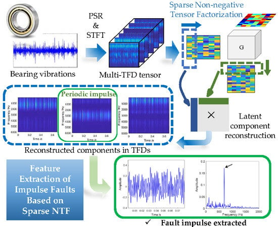
3. Feature Extraction Method of an Impulse Fault

At the inchoate stage of the machinery fault, the weak characteristic components, inundated with a large amount of background noise, carry the information of certain damages and require accurate extraction. For single-channel vibration signals, this section proposes an effective strategy that employs both the phase space reconstruction and the sparse non-negative tensor factorization to tackle the issue of weak impulse feature extraction.

3.1. Principle of Phase Space Reconstruction

The PSR is based on the conception that the correlated components within a dynamic system affect and determine the behavior of every single component, as the separated component incorporates the information from other components equally. By observing one component with different time delays, PSR is capable of determining the dimensionality of the system’s attractor.

Consider the one-dimensional vibration signal $x(n),(n=1,2,\dots ,N)$; it can be reorganized as several overlapping segments,

$$x(n)=\left(S_1^m,S_2^m,\dots ,S_r^m\right),$$

(19)

$$r=\frac{N-m}{\tau }+1,$$

(20)

where $S_i^m(i=1,2,\dots ,r)$ denotes the phase point vector, $\tau$ represents the time delay between two consecutive vectors, and m is the dimension of the vector (also called embedding dimension). Thereupon, with the help of PSR, the original sequence $x(n)$ can be reconstructed into a two-dimensional matrix or phase space, $X\in {ℝ}^{m\times r}$,

$$X=\left[\begin{array}{cccccc}{x}_1& x_{1+\tau }& \cdots & x_{1+k\tau }& \cdots & x_{1+(r-1)\tau }\\ x_2& x_{1+\tau +1}& \cdots & x_{1+\tau +1}& \cdots & x_{1+(r-1)\tau +1}\\ ⋮& ⋮& \ddots & ⋮& \ddots & ⋮\\ x_m& x_{1+\tau +(m-1)}& \cdots & x_{1+k\tau +(m-1)}& \cdots & x_{1+(r-1)\tau +(m-1)}\end{array}\right],$$

(21)

where the last element of the original signal is given by $x_{1+(r-1)\tau +(m-1)}=x_N$.

In PSR method, the time delay $\tau$ and the embedding dimension m are crucial to the accuracy of the reconstructed phase-space attractor. For time series, the phase space vector may fail to represent the local feature of the original signal if m is too small, while conversely, an embedding dimension that is too high will cause unnecessary redundancy and costly computation. Similarly, an inappropriate time delay may bring uncorrelatedness to different signal segments.

When local damages occur in the bearing, a series of periodic impulses will be excited, reflecting the fault information. The impulse response signal that attenuates in its natural period is the major object of feature extraction. Given a noisy impulse series, as shown in Figure 1, it is apparent that, the embedding dimension should be greater than the impulse period T, so that every phase will incorporate at least one impulse component. In other words, the m-point embedding dimension is subject to $m>f_s\times T$ or $m>f_s/f_i$, where T is the period of impulses in seconds and $f_s$ represents the sampling rate. In practice, $f_i$ cannot be determined in advance, while the revolving speed $f_r$ is easily accessible. Thus, the restraint can be based on $f_r$ to formulate $m>3\times f_s/f_r$, which also takes into account the theoretical characteristic frequency of bearing faults. Moreover, as STFT is used to perform on each phase point vector in the next step, the length of m can be taken as the power of two out of the efficiency in calculation.

As for the time delay, in consideration of the fact that the adjacent phase point vectors should incorporate the elements of the same impulse, $\tau$ is limited within the interval $[\frac{f_s}{f_r},m]$.

Overall, the empirical criteria can be given as follows:

$$\{\begin{array}{l}m=2^{\mathrm{int}({\log }_2(\frac{3f_s}{f_r}))+1},\\ \frac{f_s}{f_r}\le \tau \le m,\end{array}$$

(22)

where $\mathrm{int}(\cdot )$ denotes the rounding operation. Nevertheless, the signal quality definitely affects the spectrum analysis. In application, a further expanded m is also suggested for a signal with low signal to noise ratio, and the extension depends on the computing power.

3.2. Time-Frequency Distribution Construction

The time-frequency analysis techniques, including short time Fourier transform, wavelet transform, and Wigner distribution, provide solutions to mapping vibration signals on a time-frequency plane that incorporates the information from both time-domain and frequency-domain. Due to the convenient operation and good interpretability, STFT is employed to obtain the time-frequency distributions for every signal segment (or phase point vector), as discussed in the previous section.

STFT, in essence performing Fourier transform on the windowed signal segments, is defined in discrete form as follows:

$$STF{T}_x(n,m)={\displaystyle \sum _{k=nT}^{nT+N-1}x(k)w(k-nT)e^{-j\frac{2\pi km}{N}}}$$

(23)

where n, m represents the index of time sequence and frequency sequence, T denotes the sliding interval of the window $\omega (k)$, and N is the window length.

As for the window function, to strike a balance between the frequency resolution and the energy leakage, let us select the Hanning window. Yet subject to the Heisenberg uncertainty principle, the pitfall of STFT is the inevitable tradeoff between time and frequency resolution, for which an appropriate width of the window function should be determined to obtain the best time-frequency concentration. With respect to the existing norm-based measures, such as Rényi entropy, and Jones–Parks norm ratio, the Stankovic measure integrates the window energy with the norm of STFT spectrogram to provide an automatic determination of the best window length [27]. This concentration measure is given by

$$H(N)={\left({{\displaystyle \sum _{n=1}^N{\displaystyle \sum _{m=1}^N\left(\frac{1}{E(N)}|STFT(n,m){|}^2\right)}}}^{\frac{1}{2}}\right)}^2,$$

(24)

where the window energy can be written simply using the window function:

$$E(N)={\displaystyle \sum _{k=0}^{N-1}|\omega (k){|}^2}.$$

(25)

In this way, the Stankovic measure finds an optimal window length N when H(N) reaches a minimum. As a shorter window has less energy and a higher value of H(N), while a longer window does the opposite, the introduction of E(N) seemingly strikes a balance between the measure of short windows and long windows. We finally select the length N, according to Stankovic measure, but empirically at which the slope of H(N) starts to turn flat.

With the help of STFT, all column vectors in the phase space are transformed into multiple TFDs, which are then stacked up to create a three-way tensor. By synthesizing the PSR technique and STFT, the vibration signal is circularly and completely utilized to generate a third order time-frequency representation.

3.3. Non-Negative Time-Frequency Tensor Analysis

Conventional matrix factorization methods, including independent component analysis, singular value decomposition, etc., only serve in the context of two-way expressions. However, tensor factorization is effective in the application of multi-way (or high-order) data analysis and possesses great potential in sparse representation. Moreover, the nonnegativity constraints can be introduced to enhance the interpretability of the decomposed factors, while the sparsity constraints improve the local-based representation.

As the fundamentals of SNTF algorithms have been discussed, we are interested in the decomposed factors derived from the time-frequency tensor, as illustrated in Figure 2. By the virtue of the tensor factorization method, we obtain the following factors: The frequency matrix $A$, the time matrix $B$, and the phase matrix $C$. The matrix $C$ implies the proportion of the phase space information reserved in the corresponding feature subspace (or source component), e.g., vector $c_j$, implies which phase (of Q) is the most dominant for consisting the jth latent component.

Based on the decomposed factors, we rebuild the time-frequency distributions separately by performing the product of the vector from the frequency matrix and the time matrix. Thereupon, we have multiple (the number of TFDs is up to the reduced-dimensionality index $J$) reconstructed TFDs that are principally correlated to the latent component:

$$TF{D}_s=a_s{b}_s{}^T,(s=1,2,\dots ,J).$$

(26)

On these reconstructed TFDs, we perform the inverse short time Fourier transform (ISTFT) to compute the represented signal waveforms, which can be regarded as the principal components or source components of the original high-order data.

STFT is an invertible transform based on the discrete Fourier transform (DFT). ISTFT starts with the inverse DFT (IDFT) to recover a previously windowed frame, obtaining $\tilde{x}(n)$:

$$\tilde{x}(n)=={\displaystyle \sum _{k=nT}^{nT+N-1}STF{T}_x(n,m)e^{+j\frac{2\pi km}{N}}}.$$

(27)

However, discontinuities may appear between different recovered frames after IDFT, for which another windowing operation should be performed to defeat the problem. Hristo introduced a synthesis window $v(k)$ to every $\tilde{x}(n)$, which is thoroughly demonstrated in [6].

Obviously, the vibration signals collected from the machinery equipment are generally a mixture of status components, weak impulse components, and severe interference. As a result, signs of damage can hardly be recognized in either the time domain or frequency domain. However, the above strategy may efficiently reconstruct the original signal with less background noise. Based on the above knowledge, we assume that SNTF decompose the multi-TFD tensor into the linear sum of these factors: The feature subspace of periodic vibration, the feature subspace of noise, the feature subspace of other interference, and other subspaces of latent signals. To take it one step further, envelope demodulation is employed in order to extract the impulse feature within the signal, whereupon the characteristic frequency with an implication of fault should be presented in the corresponding envelope spectrum, which is difficult to realize using the conventional feature extraction methods.

3.4. Feature Extraction Method for Vibration Signals Based on Sparse Non-Negative Tensor Factorization

Based on the above elaboration, a novel feature extraction method for vibration signals is proposed. The method combines the merits of the PSR technique and the SNTF model, to effectively extract the fault feature of periodic impulses in the vibration signals. The overall procedure is concluded in Algorithm 1 given as follows:

Algorithm 1: Feature Extraction Method for Vibration Signals Based on SNTF

Step 1. The original one-dimensional signal $x(n)$ is converted into a two-dimensional phase space $X$ by the PSR technique.

Step 2. Perform STFT on the phase point vectors to acquire multiple time-frequency distributions.

Step 3. Permutate the multiple TFDs to generate a third-order tensor $\underset{\_}{Y}$.

Step 4. Select a reduced-dimensionality index $J$, and employ the SNTF-HALS algorithm to decompose the above tensor $\underset{\_}{Y}$. This step returns the frequency matrix $A$, the time matrix $B$, and the phase matrix $C$.

Step 5. The reconstructed TFDs are obtained by $a_s{b}_s{}^T,(s=1,2,\dots ,J)$, and the principal components (waveforms) are restored by ISTFT.

Step 6. Feature extraction. For a selected waveform, envelope demodulation is used to capture the characteristic frequency of certain damages.

The method is also visualized as a flow chart as presented in Figure 3.

4. Experiments on Feature Extraction of Machinery Faults

This section provides different experimental cases for evaluating the effectiveness of the proposed model. Section 4.1 and Section 4.2 offer two case studies on the benchmarked bearing datasets. Comparisons to other feature extraction models, including MCKD, SVD, and maximum spectrum kurtosis (MSK) are attached. The experiment on a swashplate piston pump is given in Section 4.3.

4.1. Feature Extraction of Impulse Fault on Bearing Dataset—Case 1

In order to validate the effectiveness of the proposed method, the bearing dataset provided by the University of Cincinnati was adopted for analysis [28]. The vibration signals were measured over the lifetime of the bearings until failure. Accordingly, we selected the data at the stage of incipient failure for validation and further analysis.

4.1.1. Experimental Settings

The experimental platform is shown in Figure 4, which consists of a transmission shaft, an AC motor, and 4 Rexnord bearings. A radial load of 2721.6 kg was applied on bearing 2 and 3 as a whole. The vibration signals were collected via PCB 353B33 accelerometers (PCB Piezotronics, Depew, NY, USA) installed on bearing housing. The data acquisition module was NI DAQ 6062E (National Instruments, Austin, TX, USA). Each record consisted of 20,480 points, with a sampling rate of 20 kHz. Other relevant experimental settings are concluded in

Table 1. Experimental settings of case 1.

Bearing Model	Running Speed	Sampling Rate	Fault Position	Characteristic Frequency
Rexnord ZA-2115	2000 RPM	20,000 Hz	Outer Ring	236.9 Hz

.

Specifically, the test signals were recorded during 12 February and 19 February 2004, when a failure occurred after over 100 million cycles causing a crack in the outer race of bearing 1. With the purpose of extracting the impulse feature in the signals at the stage of incipient faults, we examined the record for the 1st channel at 03: 42, 16 February 2004 (74 h before the end of the experiment), as shown in Figure 5.

4.1.2. Feature Extraction Based on SNTF

Based on the feature extraction method proposed above, we first reconstructed the phase space for the selected data. The length of the signal $x(n)$ was 20,480. With the speed at 2000 RPM, we obtained the embedding dimension m at 2¹¹ (2048), and the time delay $\tau$ at 600. The number of the phase point vectors was 31 (rounded down for the consistency in vector length). Accordingly, the reconstructed phase space $X\in {ℝ}^{2048\times 31}$ was derived.

When applying STFT to the phase point vectors of $X$, the width of tye Hanning window was set to 53. Thereupon, we acquired the three-way time-frequency data ($2048\times 2048\times 31$), on which the modulus operation was performed to obtain a non-negative time-frequency tensor ${\underset{\_}{Y}}_{tf}\in {ℝ}^{2048\times 2048\times 31}$.

Then, we set the reduced-dimension index $J$ at 3, knowing that the two high-frequency resonance bands in the spectrum (see Figure 5b) could be separated from the low-frequency component using SNTF. We let the sparseness regulation parameter $\alpha$ be 0.20, and performed the SNTF-HALS method to factorize the tensor ${\underset{\_}{Y}}_{tf}$ into three sparse nonnegative matrices: $A\in {ℝ}^{2048\times 3}$, $B\in {ℝ}^{2048\times 3}$, and $C\in {ℝ}^{31\times 3}$. $A$ and $B$ respectively, indicate the data distributions in frequency domain and time domain, as presented in Figure 6, where we separately plotted them as curves.

Based on the two factors, three TFDs (see Figure 7) were reconstructed via $a_s{b}_s{}^T,(s=1,2,\dots ,J)$, mentioned previously in Section 3.4. As a result, evident correlations exist between the factors and the TFDs. For example, the frequency-wise component at around 1000 Hz in reconstructed TFD 1 (Figure 7a) matches with the peak in the first graph in Figure 6a; both reconstructed TFD 2 and TFD 3 incorporate the prominent component at around 4200 Hz, which correspond with the trends of the 2nd and 3rd curves in Figure 6a.

From the figures above we can see that the periodic impulse can be found in each TFD along the time axis and that this feature is more evidently suggested in the third TFD. In order to extract such a frequency component, we perform the inverse STFT on the third TFD to recover the latent component signal. Then the envelope demodulation is applied to generate the corresponding envelope waveform and spectrum, as presented in Figure 8.

According to the envelope spectrum, the frequency component at 234.4 Hz is prominent, which can be identified as the characteristic frequency of the outer race fault of the bearing. Specifically, as the theoretical fault frequency is calculated with the hypothesis of rollers’ pure rolling, the deviation is partly due to the sliding of the rollers. With this result, the efficacy of the feature extraction method based on Sparse NTF is revealed.

4.1.3. Comparisons with Other Methods

In order to verify the effectiveness of feature extraction, some representative models were adopted for comparisons.

Maximum correlated kurtosis deconvolution (MCKD) is one of the mainstream algorithms for revealing specific impulse series from a signal and is used for analyzing the same vibration signal.

First, based on the sampling rate fs of 20,000 Hz and the characteristic frequency, extracted previously at 234.4 Hz (0.0043 s), we derived the deconvolution period Tp at 86 (rounded). Then, the length of the filter L also required determination. For finding a best L, we set a loop interval in calculation, e.g., 100 to 500, to locate the one with a maximum correlated kurtosis. In this case, L was 400.

The latent impulses extracted by MCKD are presented in Figure 9. The frequency spectrum shows the characteristic frequency and its harmonic. However, it also contains more irrelevant components as compared to the SNTF envelop spectrum. Another drawback of MCKD is that it requires an accurate period Tp in advance. A deviation between the thereotical characteristic frequency and the authentic one might produce undisirable results.

Next, we performed the feature extraction based on singular value decomposition (SVD), which has extensive applications in the field of signal processing. In essence, SVD is a generalization of eigenvalue decomposition and pertains to matrix analysis methods. To employ this method, we first consecutively selected 2048 points of data from the vibration signal, and then converted the data into a Hankel matrix, $H\in {ℝ}^{2019\times 30}$, with 30 row vectors (similar to PSR but with a time delay of 1).

$$H={\left[\begin{array}{c}{s}_1^m\\ s_2^m\\ ⋮\\ s_j^m\\ ⋮\\ s_{30}^m\end{array}\right]}^T={\left[\begin{array}{cccc}{x}_1& x_2& \cdots & x_{2019}\\ x_2& x_3& \cdots & x_{2020}\\ ⋮& ⋮& \ddots & ⋮\\ x_j& x_{j+1}& \cdots & x_{j+2018}\\ ⋮& ⋮& \ddots & ⋮\\ x_{30}& x_{31}& \cdots & x_{2048}\end{array}\right]}^T.$$

(28)

With the help of SVD, we obtained the following singular values: ${\sigma }_1\ge {\sigma }_2\ge {\sigma }_3\dots \ge {\sigma }_{30}$, which reveal the distribution of relevant signal and irrelevant interference. After employing the greatest three singular values for signal reconstruction, the frequency band of 4000 to 5000 Hz was restored, as shown in Figure 10a. Eventually, we performed the Hilbert transform to derive the envelope spectrum, as presented in Figure 10b. Similarly, the fault characteristic frequency was also extracted in the envelope spectrum, while the feature is less evident than the previous methods.

Finally, the maximum spectrum kurtosis (MSK) method was also adopted to extract the fault feature. Based on STFT, the central frequency and the resolution of the optimal bandpass filter can be obtained. The central frequency $f_{ctr}$ is selected when the value of kurtosis reaches a maximum, and the resolution $\Delta f$ is determined by the sampling rate and the window width; i.e., $\Delta f=2f_s/N_w$. We used a segment of 2048 points of the original signal and set the width of Hanning window at 45, from which we derived $f_{ctr}$ at 3750 Hz and $\Delta f$ at 663 Hz, as shown in Figure 11a. Thus the characteristic frequency band of (3087 Hz, 4413 Hz) was accessed and thereupon employed for envelope demodulation.

As presented in Figure 11b, a weak signature of the fault characteristic frequency is found in the envelope spectrum, but almost buried by other interferences. This finding suggests that the maximum spectrum kurtosis method is less effective in this application, compared to the SNTF methods.

Overall, the experimental results indicate that the MCKD is insufficient, as multiple peaks mix with the fault frequency and its harmonics in the spectrum, which can be attributed to the inaccuracy in the deconvolution period and the high sensitivity of correlated kurtosis under non-gaussian noise. MSK, which adaptively selects a frequency band with maximum kurtosis for demodulation, exhibits less satisfactory results with more interfering low-frequency components (e.g., 118 Hz and 175 Hz). The work in [5] combines the above two methods to obtain more a prominent kurtogram, but the issue of MCKD is not comprehensively illustrated. As for SVD-based extraction, the result presents dominant but irrelevant peaks (e.g., 118 Hz) besides the fault frequency, indicating that the method needs improvement in both the selection and the interpretability of singular subspaces to avoid introducing redundancy. Between the three models, SVD obtains relatively better results in this case.

Apart from the spectrum with a distinct fault frequency in Figure 8, other indications also present the advantages of our proposed method. SNTF decomposes the multi-TFD tensor into a few low-rank representations that embody the vibrations with different characteristics. The sparseness constraint plays a role in promoting the parts-based feature, as can be found in the reconstructed TFDs. Interpretability is improved by virtue of the non-negativity constraint, as the non-zero elements of SNTF decomposition are all positive values, allowing only additive combinations, rather than subtractions that occur in SVD.

4.2. Feature Extraction of Impulse Fault on Bearing Dataset—Case 2

To further verify the effectiveness of the proposed method, we also analyzed the bearing data from the Case Western Reserve University, which has been extensively used for the verification of diagnostic models. Smith et al. presented a benchmarked study of bearing diagnotics with this dataset and divided the bearing data into three categories—“obivious,” “weak,” and “cannot be diagnosed” [29]. Specifically for Case 2, we would like to test our model on the bearing data catagorized as a “weak” fault.

4.2.1. Experimental Settings

The experiment was conducted using a 1.5 kW motor (Reliance Electric Motors, Hudson, WI, USA) and a dynamometer (Reliance Electric Motors, Hudson, WI, USA), as presented in Figure 12. Data was collected using a 16-channel DAT recorder at 12,000 samples per second. The fan-end bearing fault data was selected for analysis. The single-point fault (0.35 mm in diameter, 0.28 mm in depth) was created via electro-discharge machining on the inner raceway. For brevity, we summarize the relevant experimental settings in

Table 2. Experimental settings of case 2.

Bearing Model	Running Speed	Sampling Rate	Fault Position	Characteristic Frequency
SKF 6203-2RS	1730 RPM	12,000 Hz	Inner Ring	143.2 Hz

, and Figure 13 shows the selected data in waveform and frequency spectrum.

4.2.2. Feature Extraction Based on SNTF

First, a phase space containing different time-delay segments can be built from the original time series (24,800 samples). Based on the criteria for choosing the embedding dimension, we extended the m at 2¹³ (8192) points, considering the signal in that case contained more complex components. Time delay $\tau$ was taken by half length of m at 4096. Accordingly, five phase point vectors were obtained and combined as a new phase space, $X\in {ℝ}^{8192\times 5}$.

Second, STFT was performed on each phase vector to generate five TFDs. In similar way, a three-way non-negative time-frequency tensor, ${\underset{\_}{Y}}_{tf}\in {ℝ}^{8192\times 8192\times 5}$, was obtained.

Next, we applied HALS-SNTF to decompose the tensor. As the index $J$ determines the low rank of the decomposed factors, knowing that the frequency spectrum (see Figure 13b) incorporates four distinct resonance peaks, it is reasonable to assume the four peaks could be separated from the low-frequency component by SNTF and to assign five to $J$. The sparseness regulation parameter $\alpha$ remains at 0.20. Then, the tensor, ${\underset{\_}{Y}}_{tf}\in {ℝ}^{8192\times 8192\times 5}$, was decomposed using HALS-SNTF into three factors. We visualized the frequency matrix and time matrix in Figure 14.

As the frequency componet $a_s$ and the time component $b_s$ share one-to-one correspondence, five TFDs were reconstructed via $a_s{b}_s{}^T,(s=1,2,\dots ,5)$, as shown in Figure 15. It is worth mentioning that a single component within a factor might share interactions with other components. By “one-to-one correspondence,” we presume that the frequency component $a_s$ is characterized by time component $b_s$ and that the most dominant feature can be indicated by the frequency distribution of $a_s$.

From the above TFDs, we can see that the original time-frequency information held within the tensor is separated along the frequency axis into the five feature subspaces. In a sense, the vibration information within a specific frequency band is separated by SNTF.

Then we attempted to recover the time-domain waveforms from the above TFDs for feature extraction. ISTFT turns the TFD into a time series, on which the envelop waveform and envelope spectrum are then calculated. The results were derived for every TFD, and we present the opitimal two in Figure 16.

In Figure 16c we clearly see that the envelope spectrum extracts some major components, including the runing speed fr, the characteristic frequency fc (143.6 Hz) and the harmonics of fc. Specifically, the periodic impulses relating to the inner ring damage are accompanied with an intrinsic oscillation dominated by the resonance frequency at around 3200 Hz.

More components can be found in Figure 16d; e.g., the running speed and its harmonics. Additionally, the modulation on the fault frequency is obvious. We attribute the phenomena to the relatively lower interval of frequency band. Even so, the fault-induced impulse feature is successfully extracted.

4.2.3. Comparison and Analysis

For verification, we also conducted the comparisons with MCKD, SVD, and MSK for case 2.

In the MCKD model, the deconvolution period is given at 84 (the sampling rate is 12,000 Hz and the fc is 143.6 Hz) and the length of MCKD filter is 300. The periodic train of impulse is extracted, prominent in the filtered waveform, as can be seen in Figure 17. Still, the frequency spectrum does contain the characteristic frequency of an inner ring fault, fc and its harmonics, but it is relatively more interfered by irrelevant components compared to the SNTF results.

In the SVD model, a Hankel matrix was built, based on the one-dimesional vibration signal for decomposition. Then, the components with large singular values were restored from the right singular vector and the left singular vector, which were further processed via envelope analysis, as displayed in Figure 18. We can see that the spectrum exposes the runing speed frequency fr, the characteristic frequency fc, and other interference. The fault feature was extracted but not so prominently as by the SNTF model.

In the MSK model, the central frequency $f_{ctr}$ appears at 3375 Hz, level five, with a maximum kurtosis as presented in Figure 19a, and the frequency bandwidth $\Delta f$ is thereby obtained at 750 Hz. Thus, the signal within the band of from 2526 Hz to 4125 Hz is filtered and selected for envelope demodulation. From the envelope spectrum in Figure 19b, we can see that multiple peaks stand out, including the characteristic frequency of inner ring fault, fc. As this impulse component is affected by a few other insignicant components, we hold that the MSK method is also less effective in this case.

Based on the comparative studies in Section 4.1 and Section 4.2, we can see that the SNTF-based method has evidently better performance of fault feature extraction, the results of which indicate that periodic impulses can be extracted in one of the feature subspaces. An important advantage rooted in our SNTF-based framework is the utilization of multiple TFDs, which allows comprehensive observations of a single vibration signal, despite the varying degrees of impulse fault and the changing forms of noise in different time intervals. Conventional approaches to feature extraction consider a single time-frequency spectrogram [8,30], which might receive better results after improvement.

4.3. Experiment on the Swashplate Axial Piston Pump

Piston pumps are extensively used in aerospace, marine, automotive and other industries. Due to the compact structure and complex components, a piston pump integrates both reciprocating and rotating motion and therefore generates a large amount of vibration. As a result, the collected signals are inundated with noise interference containing multiple excitations. In this section, we analyze the vibration signals acquired from the swashplate axial piston pump to verify the performance of the proposed method.

4.3.1. Experimental Settings

The schematic of our experimental test rig is presented in Figure 20, which is constructed with an AC motor, shaft couplings, a gearbox, and an axial piston pump. The pump is driven by the motor with a speed-increasing gearbox. Typically, the thrust ball bearing and the swashplate are designed for the reciprocating motion of the pistons, which increases the output pressure.

To mimic the bearing damage, a spalling defect on the ring of the thrust ball bearing was manufactured using electro-discharge machining, as presented in Figure 21. Excited by the damage of the bearing, the periodic impulse vibration will transfer to the housing of the pump through the main shaft and a deep groove ball bearing on the left end. We acquire such compound vibrations via the accelerometers (PCB Piezotronics) mounted in the radial direction of the ball bearing. The signals are collected using NI 9234 data acquisition module. Other experimental settings are summarized in

Table 3. Relevant experimental settings.

Bearing Model	Running Speed	Sampling Rate	Fault Characteristic Frequency
D8111Q	3415 RPM	25,600 Hz	689.9 Hz

.

4.3.2. Feature Extraction Based on SNTF

Given the cost of computation, we only select the sampled signal for further analysis, which is segmented at the length of 20,480 points. Figure 22 provides the waveform and spectrum of the original signal during 0–0.08 s.

Next, we convert the one-dimensional signal to a two-dimensional phase space representation by virtue of PSR method. With the sampling rate of 25,600 Hz and the speed of 3415 Hz, the embedding dimension m is 2048, and the time delay $\tau$ is set to 1024. Therefore, a total of 19 phase point vectors are generated, creating a data matrix of $2048\times 19$.

On the basis of the Stankovic principle, we empirically choose for the Hanning window, the width of 31 where the gradient of the concentration measure H(N) turns from steep to flat. Then, STFT is performed on phase point vectors to find the time-frequency distributions, which are arranged in a three-dimensional coordinate system to form the multi-aspect data tensor ${\underset{\_}{Y}}_d\in {ℝ}^{2048\times 2048\times 19}$.

Based on the HALS-SNTF algorithm, as major peaks in the frequency spectrum are found at 1695 Hz, 4616 Hz, and 8094 Hz, the reduced-dimension index is set to three, and the data tensor is decomposed further into factor matrices, within which we are interested in the frequency matrix $A$ and the time matrix $B$. By the vector product $a_s{b}_s{}^T,(s=1,2,3)$, three reconstructed TFDs are obtained, respectively, corresponding to three different feature subspaces, as provided in Figure 23a–c.

Generally, the vibration signal of a faulty ball bearing can be regarded as a compound signal with amplitude modulation. More specifically, it is the periodic impulse (the signal of a certain fault) that modulates the system’s resonance signal. From the TFDs in Figure 23, we can see that the periodic feature in the time axis is most prominent in TFD 2, and this feature lies in the presence of the resonance frequency at around 4300 Hz and 8500 Hz. Whereupon, to extract the fault feature, we chose TFD 2 to perform ISTFT and envelope demodulation successively. The results are presented in Figure 24.

The envelope spectrum in Figure 24b extracts the frequency of 687.5 Hz, which is consistent with the theoretical fault frequency of the thrust bearing. For comparison, the envelope spectra of the reconstructed TFD 1 and TFD 3, are presented in Figure 25. They do contain the fault frequency component, but they are apparently less observable than the spectrum in Figure 24.

From the above results, the impulse feature of the vibration signal is finally extracted. Thereupon, we can confirm that the feature extraction method based on SNTF is verified efficacious for primary applications in the field of machinery fault diagnosis.

5. Conclusions

The vibration signal of rotary machinery with impact faults is generally a mixture of multiple sources, in which the characteristic component revealing the latent impulses, is often weak and difficult to detect. Although many feature extraction techniques have been put forward to accurately identify fault feature hidden in the signals, such as SVD, MSK, MCKD, etc., those methods only serve in the context of two-dimensional representation. Their applications are limited when confronted with naturally high-order data. Another issue is that the increasing complexity of modern machinery has led to the growing difficulty for fault diagnosis due to multi-excitations and compound interferences. With the purpose of handling these issues, we propose a novel strategy of fault feature extraction for vibration signal based on sparse nonnegative tensor factorization.

SNTF is endowed with the ability of decomposing the multi-TFD tensor into meaningful low-rank representations, which comprise vibrations of different characteristics. The utilization of multiple TFDs allows comprehensive observations of a single vibration signal despite the time-varying interferences. As we impose the sparseness constraint to the NTF model, the sparsity level of the factors is improved, and the reconstructed components are less interfered by noise. The implementation of this strategy on the experimental signals of the bearing dataset has indicated the effectiveness of the SNTF-based feature extraction. The results of comparisons to other representative methods also suggest that the proposed method possesses better performance of feature extraction. Pragmatically, we carried out an experiment on a swashplate piston pump test rig, in which the impulse feature of the vibration signal was successfully extracted. Therefore, the proposed method is verified feasible in practice and can be identified as of great importance for vibration signal analysis in the field of mechanical health management.

Further research might further explore a more adaptive approach for the determination of window length in STFT. Also, it would be interesting to see the effect of applying NTF to fault diagnosis for a more complex rotary machine.

References

1. Randall, R.B.; Jérôme, A. Rolling Element Bearing Diagnostics—A Tutorial. Mech. Syst. Signal Process. 2011, 25, 485–520. [Google Scholar] [CrossRef]
2. Chen, G.; Fenglin, L.; Wei, H. Sparse Discriminant Manifold Projections for Bearing Fault Diagnosis. J. Sound Vib. 2017, 399, 330–344. [Google Scholar] [CrossRef]
3. Adamczak, S.; Krzysztof, S.; Mateusz, W. Comparative Study of Measurement Systems Used to Evaluate Vibrations of Rolling Bearings. Procedia Eng. 2017, 192, 971–975. [Google Scholar] [CrossRef]
4. Tian, J.; Carlos, M.; Michael, H.A.; Michael, P. Motor Bearing Fault Detection Using Spectral Kurtosis-Based Feature Extraction Coupled with K-Nearest Neighbor Distance Analysis. IEEE Trans. Ind. Electron. 2016, 63, 1793–1803. [Google Scholar] [CrossRef]
5. Jia, F.; Yaguo, L.; Hongkai, S.; Jing, L. Early Fault Diagnosis of Bearings Using an Improved Spectral Kurtosis by Maximum Correlated Kurtosis Deconvolution. Sensors 2015, 15, 29363–29377. [Google Scholar] [CrossRef] [PubMed]
6. Zhivomirov, H. On the Development of STFT-analysis and ISTFT-synthesis Routines and their Practical Implementation. TEM J. 2019, 8, 56–64. [Google Scholar] [CrossRef]
7. Rubini, R.; Meneghetti, U. Application of the Envelope and Wavelet Transform Analyses for the Diagnosis of Incipient Faults in Ball Bearings. Mech. Syst. Signal Process. 2001, 15, 287–302. [Google Scholar] [CrossRef]
8. Lin, L.; Lei, S.; Fei, L.; Ben, N.; Guanghua, X. Sparse Envelope Spectra for Feature Extraction of Bearing Faults Based on Nmf. Appl. Sci. 2019, 9, 755. [Google Scholar]
9. Leng, Y.; Zheng, A.; Fan, S. SVD component-envelope detection method and its application in the incipient fault diagnosis of rolling bearing. J. Vib. Eng. 2014, 5, 794–800. [Google Scholar] [CrossRef]
10. Jiang, H.; Jin, C.; Guangming, D.; Tao, L.; Gang, C. Study on Hankel Matrix-Based SVD and Its Application in Rolling Element Bearing Fault Diagnosis. Mech. Syst. Signal Process. 2015, 52–53, 338–359. [Google Scholar] [CrossRef]
11. Qingbo, H.; Xiaoxi, D. Time-Frequency Manifold for Machinery Fault Diagnosis. In Structural Health Monitoring; Springer: Cham, Switzerland, 2017; pp. 131–154. [Google Scholar] [CrossRef]
12. Chaofan, H.; Yanxue, W. Multidimensional Denoising of Rotating Machine Based on Tensor Factorization. Mech. Syst. Signal Process. 2019, 122, 273–289. [Google Scholar]
13. Makkiabadi, B.; Saeid, S. Factorization Based Blind Identification and Separation of Nonstationary Seizure Signals. In Proceedings of the 16th CSI International Symposium on Artificial Intelligence and Signal Processing (AISP 2012), Fars, Iran, 2–3 May 2012; pp. 617–622. [Google Scholar]
14. Nielsen, S.F.V.; Morten, M. Non-Negative Tensor Factorization with Missing Data for the Modeling of Gene Expressions in the Human Brain. In Proceedings of the 2014 IEEE International Workshop on Machine Learning for Signal Processing (MLSP), Reims, France, 21–24 September 2014; pp. 1–6. [Google Scholar]
15. Batmanghelich, N.; Aoyan, D.; Ben, T.; Christos, D. Regularized Tensor Factorization for Multi-Modality Medical Image Classification. In Proceedings of the International Conference on Medical Image Computing and Computer-Assisted Intervention, Toronto, ON, Canada, 18–22 September 2011; pp. 17–24. [Google Scholar]
16. Wu, Q.; Liqing, Z.; Guangchuan, S. Robust Feature Extraction for Speaker Recognition Based on Constrained Nonnegative Tensor Factorization. J. Comput. Sci. Technol. 2010, 25, 783–792. [Google Scholar] [CrossRef]
17. Rafailidis, D.; Alexandros, N. Modeling the Dynamics of User Preferences in Coupled Tensor Factorization. In Proceedings of the 8th ACM Conference on Recommender Systems, Silicon Valley, CA, USA, 6–10 October 2014; pp. 321–324. [Google Scholar]
18. Zdunek, R.; Krzysztof, F.; Andrzej, W. Linked Cp Tensor Decomposition Algorithms for Shared and Individual Feature Extraction. Signal Process. Image Commun. 2019, 73, 37–52. [Google Scholar] [CrossRef]
19. Cichocki, A.; Rafal, Z.; Anh, H.P.; Shun-ichi, A. Nonnegative Matrix and Tensor Factorizations; John Wiley & Sons: West Sussex, UK, 2009; p. 338. [Google Scholar]
20. Sidiropoulos, N.D.; Lieven, D.L.; Xiao, F.; Kejun, H.; Evangelos, E.P.; Christos, F. Tensor Decomposition for Signal Processing and Machine Learning. IEEE Trans. Signal Process. 2017, 65, 3551–3582. [Google Scholar] [CrossRef]
21. Yang, D.; Cancan, Y.; Zengbin, X.; Yi, Z.; Mao, G.; Changming, L. Improved Tensor-Based Singular Spectrum Analysis Based on Single Channel Blind Source Separation Algorithm and Its Application to Fault Diagnosis. Appl. Sci. 2017, 7, 418. [Google Scholar] [CrossRef]
22. Li, G.; Lin, L.; Dan, L.; Maolin, L.; Bao, W.; Guanghua, X. The Source Separation of Multi-Channel Vibration Signal Based on Nonnegative Tensor Factorization. In Proceedings of the 10th International Conference on Communications, Circuits and Systems (ICCCAS), Chengdu, China, 22–24 December 2018; pp. 359–363. [Google Scholar]
23. Wang, F.; Shouhai, C.; Jian, S.; Dawen, Y.; Lei, W.; Lihua, Z. Time-Frequency Fault Feature Extraction for Rolling Bearing Based on the Tensor Manifold Method. Math. Probl. Eng. 2014, 2014, 2014. [Google Scholar] [CrossRef]
24. Cichocki, A.; Rafal, Z.; Shun-ichi, A. Hierarchical ALS Algorithms for Nonnegative Matrix and 3d Tensor Factorization. In Proceedings of the International Conference on Latent Variable Analysis and Signal Separation, London, UK, 9–12 September 2007; pp. 169–176. [Google Scholar]
25. Cichocki, A.; Phan, A.H.; Zdunek, R.; Zhang, L.Q. Flexible Component Analysis for Sparse, Smooth, Nonnegative Coding or Representation. In Proceedings of the International Conference on Neural Information Processing, Kitakyushu, Japan, 13–16 November 2008; pp. 811–820. [Google Scholar]
26. Cichocki, A.; Anh, H.P.; Cesar, C. Flexible HALS Algorithms for Sparse Non-Negative Matrix/Tensor Factorization. In Proceedings of the 2008 IEEE Workshop on Machine Learning for Signal Processing, Cancun, Mexico, 16–19 Octorber 2008; pp. 73–78. [Google Scholar]
27. Stanković, L. A Measure of Some Time–Frequency Distributions Concentration. Signal Process. 2001, 81, 621–631. [Google Scholar] [CrossRef]
28. Qiu, H.; Jay, L.; Jing, L.; Gang, Y. Wavelet Filter-Based Weak Signature Detection Method and Its Application on Rolling Element Bearing Prognostics. J. Sound Vib. 2006, 289, 1066–1090. [Google Scholar] [CrossRef]
29. Smith, W.A.; Robert, B.R. Rolling Element Bearing Diagnostics Using the Case Western Reserve University Data: A Benchmark Study. Mech. Syst. Signal Process. 2015, 64–65, 100–131. [Google Scholar] [CrossRef]
30. Cai, S.; Jianfeng, Q.; Zeping, W.; Chunyan, L. Feature Extraction of Rolling Bearing Incipient Fault Using an Improved SCA-Based UBSS Method. In Proceedings of the International Conference on Mechatronics and Intelligent Robotics, Kunming, China, 19–20 May 2019; pp. 994–1002. [Google Scholar]
Figure 1. Simulated signal of the impact damage.
Applsci 09 03642 g001
Figure 2. Decomposition of time-frequency tensor.
Applsci 09 03642 g002
Figure 3. The overall procedure of the sparse non-negative tensor factorization (SNTF)-based feature extraction for machinery faults.
Applsci 09 03642 g003
Figure 4. Bearing test rig and sensor placement [28]. Reproduced with permission from [28], Elsevier, 2019.
Applsci 09 03642 g004
Figure 5. The vibration signal of bearing 1 for further analysis: (a) In the waveform only a faint trace of impulse is found; (b) the spectrum contains multiple frequency components, with resonance features located at around 1000 Hz, and between 3000 Hz and 5000 Hz.
Applsci 09 03642 g005
Figure 6. Decomposed factors of SNTF: (a) Frequency matrix A; (b) time matrix B.
Applsci 09 03642 g006
Figure 7. Reconstructed time-frequency distributions based on the vector product: (a) Reconstructed time-frequency distribution (TFD) 1; (b) reconstructed TFD 2; (c) reconstructed TFD 3.
Applsci 09 03642 g007
Figure 8. Results of the envelope demodulation: (a) The envelope waveform of latent component three; and (b) the corresponding envelope spectrum.
Applsci 09 03642 g008
Figure 9. Results based on maximum correlated kurtosis deconvolution (MCKD): (a) The deconvolution signal after filtering; (b) the frequency spectrum of the deconvolution.
Applsci 09 03642 g009
Figure 10. Results based on singular value decomposition (SVD): (a) SVD-reconstructed spectrum; and (b) the corresponding envelope spectrum.
Applsci 09 03642 g010
Figure 11. Results based on maximum spectrum (MSK): (a) Kurtogram of the signal; (b) envelope spectrum of the filtered signal.
Applsci 09 03642 g011
Figure 12. Experimental test stand. Left: Motor; center: Torque transducer; right: Dynamometer.
Applsci 09 03642 g012
Figure 13. The original vibration signal: (a) The waveform incorporates a few impulses; (b) in the spectrum, prominent resonance bands stand out at around 500 Hz, 1000 Hz, 1300 Hz, and 3250 Hz.
Applsci 09 03642 g013
Figure 14. Decomposed factors of SNTF: (a) Frequency matrix A; (b) time matrix B.
Applsci 09 03642 g014
Figure 15. Illustrations of the reconstructed TFDs: (ae) Reconstructed TFD 1–5. Components lie in different frequency band after tensor factorization and reconstruction.
Applsci 09 03642 g015
Figure 16. Results of feature extraction of reconstructed TFD 2 (dominant frequency band—around 3200 Hz) and TFD 3 (dominant frequency band—within 1000 Hz): (a) Envelope waveform of TFD 2; (c) envelope spectrum of TFD 2; (b) envelope waveform of TFD 3; (d) envelope spectrum of TFD 3.
Applsci 09 03642 g016aApplsci 09 03642 g016b
Figure 17. Results based on MCKD in case 2: (a) In the deconvolution signal, impulses are revealed; (b) the frequency spectrum also captures the characteristic fault, but it is interfered.
Applsci 09 03642 g017
Figure 18. Results based on SVD in case 2: (a) The frequency spectrum of the recovered signal (2800 Hz to 3800 Hz); (b) envelope spectrum.
Applsci 09 03642 g018
Figure 19. Results based on MSK in case 2: (a) Kurtogram of the signal; (b) envelope spectrum of the filtered signal.
Applsci 09 03642 g019
Figure 20. The swashplate axial piston pump test rig.
Applsci 09 03642 g020
Figure 21. Spalling defect on the ring of the thrust ball bearing.
Applsci 09 03642 g021
Figure 22. The original signal for further analysis: (a) Waveform; (b) frequency spectrum.
Applsci 09 03642 g022
Figure 23. The reconstructed TFDs based on the SNTF factors: (a) Reconstructed TFD 1; (b) reconstructed TFD 2; (c) reconstructed TFD 3.
Applsci 09 03642 g023
Figure 24. The results of envelope analysis based on reconstructed TFD 2: (a) Envelope waveform; (b) envelope spectrum.
Applsci 09 03642 g024
Figure 25. The envelope spectra based on the reconstructed TFD 1 and 3: (a) Envelope spectrum based on the reconstructed TFD 1; (b) envelope spectrum based on the reconstructed TFD 3.
Applsci 09 03642 g025