Article

Fault Diagnosis of Rolling Bearing Based on Multiscale Intrinsic Mode Function Permutation Entropy and a Stacked Sparse Denoising Autoencoder

College of Field Engineering, Army Engineering University of PLA, Nanjing 210007, China
*
Author to whom correspondence should be addressed.
Appl. Sci. 2019, 9(13), 2743; https://doi.org/10.3390/app9132743
Submission received: 28 April 2019 / Revised: 14 June 2019 / Accepted: 2 July 2019 / Published: 6 July 2019
(This article belongs to the Special Issue Fault Diagnosis of Rotating Machine)

Abstract

:
Effective intelligent fault diagnosis of bearings is important for improving safety and reliability of machine. Benefiting from the training advantages, deep learning method can automatically and adaptively learn more abstract and high-level features without much priori knowledge. To realize representative features mining and automatic recognition of bearing health condition, a diagnostic model of stacked sparse denoising autoencoder (SSDAE) which combines sparse autoencoder (SAE) and denoising autoencoder (DAE) is proposed in this paper. The sparse criterion in SAE, corrupting operation in DAE and reasonable designing of the stack order of autoencoders help to mine essential information of the input and improve fault pattern classification robustness. In order to provide better input features for the constructed network, the raw non-stationary and nonlinear vibration signals are processed with ensemble empirical mode decomposition (EEMD) and multiscale permutation entropy (MPE). MPE features which are extracted based on both the selected characteristic frequency-related intrinsic mode function components (IMFs) and the raw signal, are used as low-level feature for the input of the proposed diagnostic model for health condition recognition and classification. Two experiments based on the Case Western Reserve University (CWRU) dataset and the measurement dataset from laboratory were conducted, and results demonstrate the effectiveness of the proposed method and highlight its excellent performance relative to existing methods.

1. Introduction

Rolling bearing is widely used and plays an important role in rotating machinery. With the increasing speeds of modern rotating machinery, the dynamic loads on bearings have become increasingly complicated and adverse [1,2]. As such, the abrasion of bearings has become an increasingly serious concern. These issues impede normal operation and may have negative safety consequences. Therefore, accurate monitoring and diagnosis of bearing working conditions is important for the normal operation of rotating machinery. However, when bearings damaged, the damage point repeatedly impacts the surface of other components in contact with it, resulting in erratic vibrations. Therefore, bearing vibration signals are often non-linear and non-stationary and contain a variety of frequency components, which distorts the signal. Bearing faults are difficult to correctly detect and effectively identify. Therefore, to improve bearing fault detection and diagnosis, it is essential to study representative feature extraction and intelligent fault pattern recognition.
Signal processing and feature extraction are crucial in fault diagnosis. To effectively manage non-linear and non-stationary signals, time-frequency analysis methods are widely used. Compared with Wigner–Ville distribution (WVD) [3], wavelet transform has been fully applied in bearing fault detection [4,5,6] because of its non-crossover term and flexible choice in wavelet function. Different wavelet bases are suitable for analyzing different time-frequency characteristics. For inexperienced researchers, choosing the wavelet base poses a considerable challenge. Empirical mode decomposition (EMD) [7] decomposes the complex signal into finite stationary intrinsic mode functions (IMFs), which is an adaptive signal processing method independent of base function. Aimed to alias EMD modes [8], ensemble empirical mode decomposition (EEMD) [9], which has effectively improved problems of EMD mode aliasing, endpoint effects, and false components, was proposed. Due to multi-scale expression and a strong adaptive ability, EEMD is suitable for processing non-linear and non-stationary signals and has been successfully applied in health detection of mechanical equipment [10]. Therefore, in our research, EEMD was used to preprocess raw signals for multi-scale analysis.
Rolling bearing vibration signals usually contain many interference frequency components, which distort the signal. Therefore, if the impact characteristics of a vibration signal can be effectively enhanced, fault features would be more accurately extracted and the diagnosis of the rolling bearing would improve. Permutation entropy (PE) [11] was proposed to detect the randomness and dynamic mutation of time series, having high computational efficiency, a stable computational value, strong anti-noise ability, and suitability for online monitoring. Therefore, PE has been widely applied in time series analysis [12,13]. Based on the complexity of the components in a mechanical system, it is necessary to conduct multi-scale analysis and processing to ensure the integrity of the local and overall information of the vibration signal. Therefore, multiscale permutation entropy (MPE) [14], considering its classification accuracy for the health of rolling bearings, was proposed to measure the complexity and randomness of time series on different scales.
Taking the extracted features as input, intelligent classification algorithms are used for fault pattern recognition. Artificial neural network (ANN) and support vector machine (SVM) are the two most commonly used machine learning methods for fault diagnosis. ANN has outstanding learning, associative storage, and high-speed optimization ability [15,16]. Wang et al. [17] used wavelet packet transform (WPT) to extract features of bearing vibration signal as input of ANN, which has achieved good fault classification accuracy. However, for non-steady and high-dimensional classification issues, there are bottlenecks, such as over-fitting due to highly strict training goals and a proneness to fall into a local optimum that restricts the performance improvement of ANN. As a statistical learning theory-based method, SVM has unique advantages in solving nonlinear, high-dimensional pattern recognition problems, especially in cases with two-class discriminating issues and fewer samples [18,19]. Zhang et al. [20] used intrinsic time scale decomposition (ITD) to calculate the Lempel-Ziv complexity of PR components to construct the feature vector as the input of SVM to accomplish the classification of different fault types, which has achieved high prediction accuracy without suffering from the influence of load variations. Liang et al. [21] utilized the sparse representation to extract sparse coefficients of both current signal and vibration signals to input the support vector machine for fault diagnosis, it showed that the method is feasible, accurate and suitable for small sample. However, SVM training is difficult when faced with multi-classification issues and large-scale training samples. But in reality, intelligent diagnosis is always based on online monitoring with inevitably large quantities of samples. If fault superposition and damage degree are considered, it is also inevitable that the number of fault modes increases considerably. Therefore, although these methods can automatically and adaptively recognize faults according to the extracted features, which significantly reduce the influence of manual experience and subjectivity in the recognition process and result, shallow learning method limits the capacity to effectively mine features in high-dimensional and non-steady data.
As the latest achievement and research focus in machine learning, deep learning methods are widely used in many fields [22,23,24,25]. Benefiting from their deep structure and the training advantages of layer-by-layer greedy learning, deep learning methods can be used to implement advanced nonlinear transformations and can automatically and adaptively learn high-order abstract features from inputs. Therefore, deep learning in intelligent fault diagnosis has attracted an increasing amount of attention. Convolutional neural networks (CNNs) [26], deep belief networks (DBNs) [27], and recurrent neural networks (RNNs) [28] have been introduced for the fault diagnosis of rotating machinery. As one of the most widely used method, stacked autoencoder [29] has attracted attention in fault diagnosis. Jia et al. [30] proposed stacked-autoencoder-based deep neural network (DNN) for roller bearing and gearbox fault diagnosis with frequency spectra after Fourier transform as inputs. Xia et al. [31] proposed an intelligent fault diagnosis approach that uses DNN based on a stacked denoising autoencoder (SDAE) for bearing diagnosis, and the results indicated that this method can extract representative features from massive unlabeled data and achieve high accuracy. Tan et al. [32] proposed an intelligent fault diagnosis model based on wavelet transform and stacked autoencoder for rolling bearing diagnosis. Muhammad et al. [33] proposed a hybrid feature pool in combination with stacked sparse autoencoder (SSAE) to effectively diagnose bearing faults of multiple severities.
By summarizing the existing researches, it is found that most related work of autoencoder in intelligent diagnosis either applies sparse autoencoder (SAE) or denoising autoencoder (DAE) alone. Although in [34], denoising sparse autoencoder was proposed through introducing both corrupting operation and sparsity constraint into a traditional autoencoder, and was applied in MNIST dataset. There are no researches that combine SAE and DAE, and study the influence of different stack order on diagnosis result. This paper proposed a hybrid autoencoder named stacked sparse denoising autoencoder (SSDAE) which combines SAE and DAE for more representative features extraction and health condition recognition. The effective fault features are extracted using a hybrid method blending EEMD and MPE. EEMD is used to preprocess the raw signals, and the screening of IMFs related to characteristic frequency is carried out. MPE of both the selected IMFs and the raw signals are obtained and fused to input into the proposed SSDAE model for training and classification.
The rest of this paper is organized as follows: Section 2 presents a fault diagnosis SSDAE model that combines EEMD and MPE, with a detailed overview of the proposed method. In Section 3, two kinds of bearing dataset are adopted to validate the effectiveness of the proposed method. The superiority of the proposed method is exhibited through some comparisons. Conclusions are drawn and future work is suggested in Section 4.

2. Proposed Fault Diagnosis Method

2.1. Overview of the Proposed Method

Figure 1 illustrates the procedure of the SSDAE-based diagnosis method presented in this paper. Collected signals are divided into training and testing samples for further processing. And in the feature extraction period, EEMD is used to adaptively decompose the raw signals for a set of IMFs. By analyzing the signal and its IMFs in frequency domain, the IMFs related to the characteristic frequency of different kinds of signals are screened. MPE of both the selected IMFs and the raw signal is calculated, and fused to form a multi-scale high-dimensional feature vector that represents the complex information used for characterizing bearing states. Finally, the fused feature vector is used as the input for the SSDA training and testing.

2.2. Signal Preprocessing Based on EEMD

Huang and Wu [9] proposed the EEMD method, in which multiple averaged noise is added to different scales of the signal. Based on the statistical randomness of the white noise, the signal components were automatically mapped to the scale plane related to the background white noise. After multiple averages, the noise was approximated to an IMF. The calculation method is as follows:
(1)
Let the raw signal be x ( t ) , and let N be the number of aggregates. Let j = 1 .
(2)
Add Gaussian white noise with amplitude coefficient k to x ( t ) . Generate a new signal x j ( t ) :
x j ( t ) = x ( t ) + k n j ( t )
(3)
Decompose x j ( t ) into a series of IMFs using the EMD method.
(4)
When m < N , repeat steps (2) and (3), but the newly added Gaussian white noise needs to be different from the previous noise. Let j = j + 1 .
(5)
After the above N decompositions, generate several groups of IMFs. Their mean values are:
c ¯ i = j = 1 N c i , j / N
where N denotes aggregates numbers and c i , j is the ith IMF from the jth decomposition. The final IMF is the N decomposition of each of the above IMFs.
When using EEMD to decompose a complex signal, it is prone to producing false IMFs that have no physical meaning. Especially in the low-frequency part of the later decomposition stage, there are more false components, and the signal interferes with the extraction of useful feature components. In this respect, Huang et al. [35] proposed an SD threshold method and a termination condition based on zero and an extreme point, and Rilling and Flandrin [36] proposed an amplitude ratio judgment method. EEMD was improved using the above methods, and the low-frequency pseudo-components generated in the later decomposition can be eliminated to a certain extent, but the noise interference components or the pseudo-components of the intermediate frequency generated by decomposition still exist. Therefore, in our research, to reduce the influence of these false components, IMF component extraction based on characteristic frequency correlation is adopted.

2.3. Feature Extraction Based on MPE

Bandt and Pompe [11] proposed PE, which is based on a comparison of adjacent data without considering the specific value of the data. PE can effectively reduce noise interference and computational complexity. The specific calculation principles are as follows:
For the time-domain signal sequence x ( i ) with length N , by reconstructing its phase space, the following time series could be obtained:
{ X ( 1 ) = { x ( 1 ) , x ( 1 + t ) , , x ( 1 + ( m 1 ) t } X ( i ) = { x ( i ) , x ( i + t ) , , x ( i + ( m 1 ) t } X ( N ( m 1 ) t ) = { x ( N ( m 1 ) t ) , x ( N ( m 2 ) t ) , , x ( N ) }
where m is the embedding dimension, and t is the time delay.
The arbitrary sequence X ( i ) = { x ( i ) , x ( i + t ) , , x ( i + ( m 1 ) t } is rearranged in ascending order as shown in Equation (4).
X ( i ) = { x ( i + ( j 1 1 ) t ) x ( i + ( j 2 1 ) t ) x ( i + ( j m 1 ) t }
If x ( i + ( j a 1 ) t ) = x ( i + ( j b 1 ) t ) exists, it is arranged according to the values of j a and j b . For example, when j a < j b is satisfied, x ( i + ( j a 1 ) t ) x ( i + ( j b 1 ) t ) . Therefore, for any sequence x ( i ) , all reconstructed vectors can obtain a set of symbol sequences.
S ( l ) = { j 1 , j 2 , j m }
where l = 1 , 2 , , m ! .
For m different symbols { j 1 , j 2 , j m } , there are m ! different permutations, which is m ! different symbol sequences.
For each symbol sequence, the probability of its occurrence is p f . Shannon’s entropy defines the PE of the symbol sequence corresponding to the k reconstruction vector of time series x ( i ) , as shown in Equation (6).
H p ( m ) = l = 1 m ! p f ln ( p f )
when p f = 1 m ! , H P ( m ) achieves the maximum value ln ( m ! ) , and H P ( m ) is standardized in turn:
H p = H P ( m ) / ln ( m ! )
The larger the H P , the more random the signal sequence, and the more dispersed the signal energy. The smaller the H P , the more regular the signal sequence, the more concentrated the signal energy, and the higher the fault probability.
On the basis of PE, Arenas et al. [14] proposed multiscale permutation entropy (MPE) to measure the complexity and randomness of time series at different scales. MPE is the PE of the time series on different scales, which adds a process of coarsening time series, as shown in Equation (8):
y λ ( j ) = 1 λ i = ( j 1 ) λ + 1 j λ x ( i )
where λ represents the scale factor and y s ( j ) represents coarse-grained data arrangement. The parameter selection considerably influences the calculation result, so before feature extraction, it is necessary to determine three important parameters: embedding dimension m , time delay t , and scale factor λ . When m is too large, the calculation of the phase space is complex, and the calculation time increases. When m is too small, the reconstructed information is insufficient for the extraction and detection of mutation signals. According to Bandt and Pompe [11], m ranges from 3 to 7. Figure 2 shows the PE values of Gaussian white noise in different embedding dimension. Figure 2 shows that the smaller the embedding dimension, the larger the PE value. Therefore, the embedding dimension should not be too small. In our experimental study, m = 5 was selected. Figure 2 also shows that the MPE of Gaussian white noise decreases monotonously with the increase in the scale factor. The relationship between PE and embedding dimension under different time delays is shown in Figure 3. It can be seen that time delay has little effect on time series, t = 1 was chosen in this paper. Scale factor λ determines the PE characteristics of the signal at the corresponding scale. Generally, as proposed in Zheng et al. [37], the maximum scale factor is usually more than 10.

2.4. Health Condition Classification Based on the SSDAE

2.4.1. Autoencoder and its Variant Algorithms

Autoencoder (AE) is a typical three-layer neural network that consists of an input layer, a hidden layer, and an output layer. As shown in Figure 4, the network structure is divided into coding and decoding processes. Mapping from input layer to hidden layer is a coding process, and the mapping from hidden layer to output layer is a decoding process. AE extracts and compresses the input features in the coding part and then restores the compressed features in the decoding part, which turns the hidden layer into another form of expression of the input.
Assume that input data is X , and the reconstructed data is X ^ , and the average reconstruction error between X and X ^ is as shown in Equation (9), where n is the number of training samples, X ^ i is the new sample reconstructed from the input, X i is the raw input, W is the weight, and b is the bias.
J ( W , b ) = 1 n i = 1 n ( 1 2 X ^ i X i 2 )
AE realizes the repetition of input through the encoding and decoding processes, in which much redundant information interferes with the extraction of useful features. To solve this problem, Bengio et al. [38] proposed a sparse autoencoder (SAE) in which a restriction condition is added to the coding process. Sparse restriction refers to the suppression of hidden layer neurons in most cases. Here, a sigmoid function is used as an activation function. The SAE adds a sparse penalty term to the loss function, and its expression is shown in Equation (10):
l = 1 m K L ( ρ | | ρ ^ l ) = l = 1 m ρ log ρ ρ ^ l + ( 1 ρ ) log 1 ρ 1 ρ ^ l
where m is the number of neurons in the hidden layer, index l represents each neuron in the hidden layer in turn, ρ is a sparse parameter, and ρ ^ l represents the average activity of the hidden layer l , and its expression is in Equation (11):
ρ ^ l = 1 n i = 1 n [ a l ( 2 ) ( x ( i ) ) ]
where a l ( 2 ) denotes the activation of hidden neurons, and a l ( 2 ) ( x ( i ) ) denotes the activation of hidden neurons x in a given input of l . The function K L ( ρ | | ρ ^ l ) has the following properties: when ρ ^ l = ρ , K L ( ρ | | ρ ^ l ) = 0 increases monotonously as the difference between ρ ^ l and ρ increases. The function K L ( ρ | | ρ ^ l ) is added to the loss function, and the loss function is then minimized, so the effects of ρ ^ l and ρ are as close as possible. The loss function of the SAE is shown in Equation (12):
J s p a r s e ( W , b ) = J ( W , b ) + β l = 1 m K L ( ρ | | ρ ^ l )
where β denotes the weight of the sparse penalty items. When the SAE extracts features, most of the neurons in the hidden layer are suppressed, and its mechanism is similar to that of a visual system. The advantage of SAE is that it can learn more representative and sparse features from the input rather than just reproduce them. Therefore, the features extracted by the SAE help improve the reliability of health condition recognition.
Denoising autoencoder (DAE) [22] is to add noise to the input and then train the network with the noised input. The training objective is to make the output as close as possible to the raw input to improve robustness of the features. The new feature h and the reconstructed data are defined in Equations (13) and (14), respectively, where s i is the activation function of coding, s d is the decoding activation function, w is the weight matrix, w ˜ is w T , b is the coding deviation, and p is the decoding deviation. Finally, the loss function of DAE is obtained as shown in Equation (15), where N is the training sample set, and θ = { w , b , p } .
h = i ( x ˜ ) = s i ( w x ˜ + b )
x ^ = d ( h ) = s d ( w ˜ h + p )
J D A E ( θ ) = x N L ( x , d ( i ( x ˜ ) ) )

2.4.2. Stacked Sparse Denoising Autoencoder

Deep learning produces excellent performance by optimizing network structure and training methods. Therefore, to recognize fault states correctly in complex working conditions for bearing fault diagnosis, it is essential to construct a deep network with a reasonable structure and excellent training methods. Bengio [29] proposed a deep learning network constructed by a stacked autoencoder that is composed of several shallow AEs. The training idea is that, through an unsupervised self-learning method, each AE is trained sequentially so that the whole network is trained. The hidden layer parameters of each AE are then stacked to construct a deep structure.
Based on the above analysis, a stacking training strategy is simpler than directly training large-scale deep network architecture, and the network training more easily converges. However, it is worth studying which features are more conducive to health condition recognition and how extracted features can be more easily classified. Therefore, in our research, to better manage the high-dimensional feature vector and extract sparse and robust features, a hybrid autoencoder, which combines SAE and DAE, is proposed.
Figure 5 depicts the construction and training process of the proposed SSDAE model; Figure 5a,b are the shallow SAE and DAE, respectively. In the training process, H i represents the hidden layer feature, W e i is the coding weight from the input layer to the hidden layer; W d i is the decoding weight from the hidden layer to the output layer; and i represents the training group. Firstly, the SAE is unsupervised trained, and the trained hidden layer parameters H 1 are used as the input of the DAE, which is also unsupervised trained. Finally, based on the stacked training parameters of the two models, a hybrid autoencoder is constructed, as shown in Figure 5c. W e 1 and W e 2 are the coding weights of the first and second layers, respectively; and W d 1 W d 2 are the decoding weights of the third and fourth layers, respectively. As shown in Figure 5d, taking the two trained hidden layers and adding a Softmax classifier, the supervised learning SSDAE model is constructed. Thus, by establishing a reasonable model arrangement order and stacking form, input features can be optimally selected and fault recognition performance can be further improved.

3. Experiments and Analysis

In this section, two experiments were constructed to prove the effectiveness of the proposed method. In Experiment 1, the Case Western Reserve University (CWRU) bearing dataset was employed. In Experiment 2, a single point and compound bearing faults experiment was designed in the rotor-bearing experimental system. For purpose of a fair comparison, three conditions are the same as follows: (1) the length of each sample is 2048 points; (2) the SSDA is trained by two-thirds of the samples, and the rest samples are utilized to test the performance; (3) each experiment runs four times to reduce the randomness.

3.1. Experiment 1: Case Western Reserve University (CWRU) Bearing Dataset

3.1.1. Dataset Introduction and Experiment Description

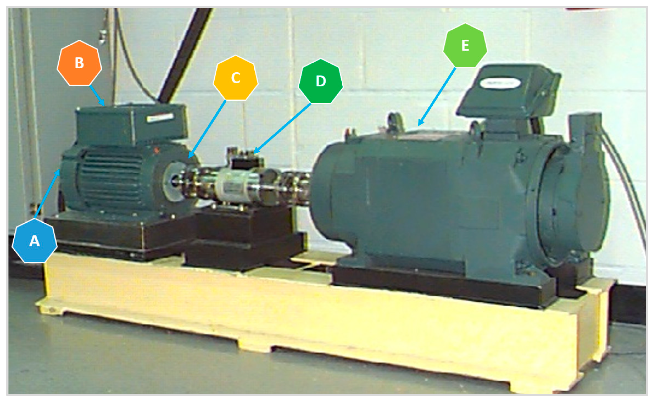
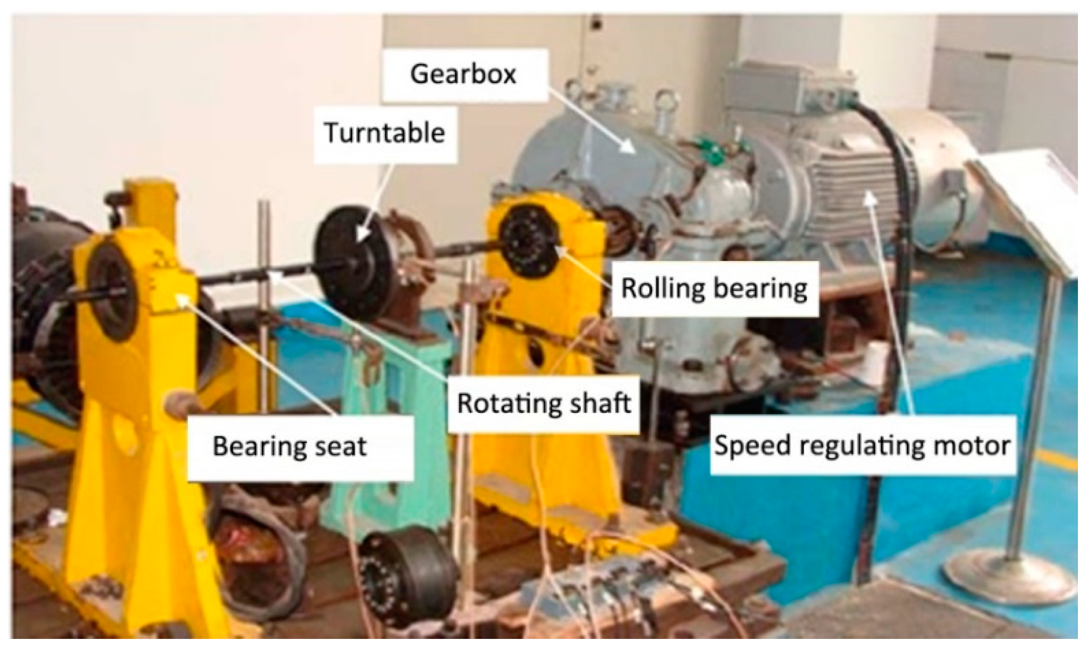
The data used in this paper for experimental validation were provided by Case Western Reserve University (CWRU), Cleveland, Ohio, USA. As shown in Figure 6, the test stand consists of an electronic motor, a torque transducer, a dynamometer, and control electronics. Single point faults were introduced to the test bearings using electro-discharge machining. Faults were set on the rolling elements, the outer races, and the inner races, and each fault bearing was installed in the test ring, which was run at a constant speed for motor loads of 0, 746, 1492, and 2238W, with motor speeds corresponding to 1797, 1772, 1750, and 1730 rpm. A more detailed introduction can be found on the CWRU Bearing Data website [39].
In this experiment, sample data were collected at 12 kHz, and detailed information is listed in 
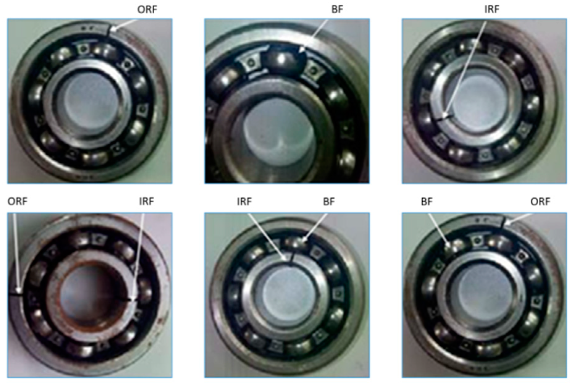
Table 1. A motor load of 746W with corresponding motor speeds of 1772 rpm was selected. Datasets, including a normal condition (N), an outer race fault (ORF), a ball fault (BF), and an inter race fault (IRF), with fault diameters of 0.18, 0.36, and 0.54 mm. and a fault depth of 0.3mm, were selected. We chose 150 samples for each defect diameter with the same fault type, in which 100 samples at a motor load of 746W were used for training, and the remaining 50 samples were used for testing. Therefore, each fault type included 450 samples; 300 samples and 150 samples of which were respectively used as training and testing samples. Detailed information on the bearing datasets is provided in Table 2.

3.1.2. Spectral Characteristic Analysis and IMFs Screening

Before processing, the raw signal was analyzed preliminarily. The rotating frequency of the shaft is 29.5Hz. According to the bearing parameters and the shaft rotating frequency, the fault characteristic frequencies of each part can be calculated [40]. The characteristic frequencies of IRF, ORF and BF are f I = 159.9 Hz, f O = 105.8 Hz and f B = 139.2 , respectively. The time domain signals of four different conditions and their spectra figures are shown in Figure 7. It can be seen the main frequency components of normal condition are concentrated within 2000 Hz, and main characteristic frequencies are 87.89 Hz, 1066 Hz and 2104 Hz, which are 3, 36 and 71 times of the frequency conversion respectively. The main frequency components of ORF are concentrated, and 2449 Hz, 2602 Hz, 2707 Hz, 2871 Hz and 3357 Hz are the main frequency components, and only 2449 Hz is the frequency doubling of the shaft rotating frequency and its characteristic frequency. The main frequency components are also concentrated in BF spectrum, 3217 Hz and 3480 Hz are the frequency doubling of the rotating frequency and its characteristic frequency. The main frequency components of IRF are multiple and scattered, and only 2742 Hz and 3539 Hz are the frequency doubling of the rotating frequency and its characteristic frequency. From the above spectrum analysis, it can be seen that only a few of the main frequency components in each state are frequency conversion and frequency doubling of their fault characteristic frequencies, and there are many interference frequencies.
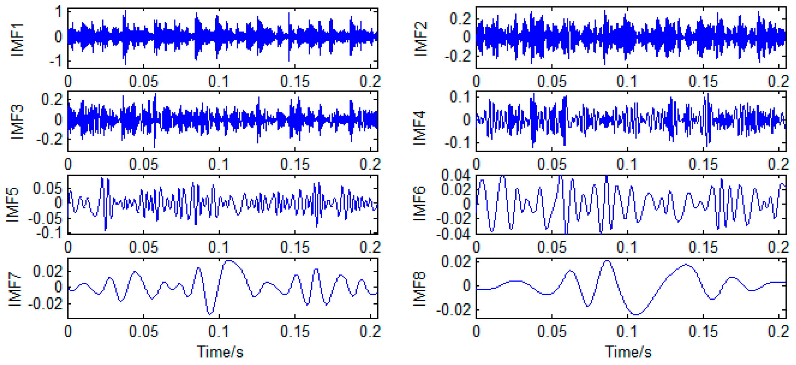
The signal samples were initially preprocessed with EEMD. Figure 8 shows IMFs of a BF signal sample. As can be deduced from the IMF waveform, the first five-order IMFs contain sufficient frequency components, and IMF6–IMF8 may be low-frequency false components. As shown in Figure 9, (a) is spectrogram of a BF sample, and (b) are the spectrogram of its eight-order IMFs. It can be seen that IMF1 to IMF5 contain the main characteristic frequency components of the raw signal from high frequency to low frequency, respectively. IMF5 is followed by low-frequency false components. So the first five-order IMFs were selected for the subsequent feature extraction.

3.1.3. Scale Factor Selection and Feature Extraction Analysis

In the PE feature extraction process, as described in Section 2.3, m was selected as 5, and t was set as 1. Moreover, the range of scale factor λ 
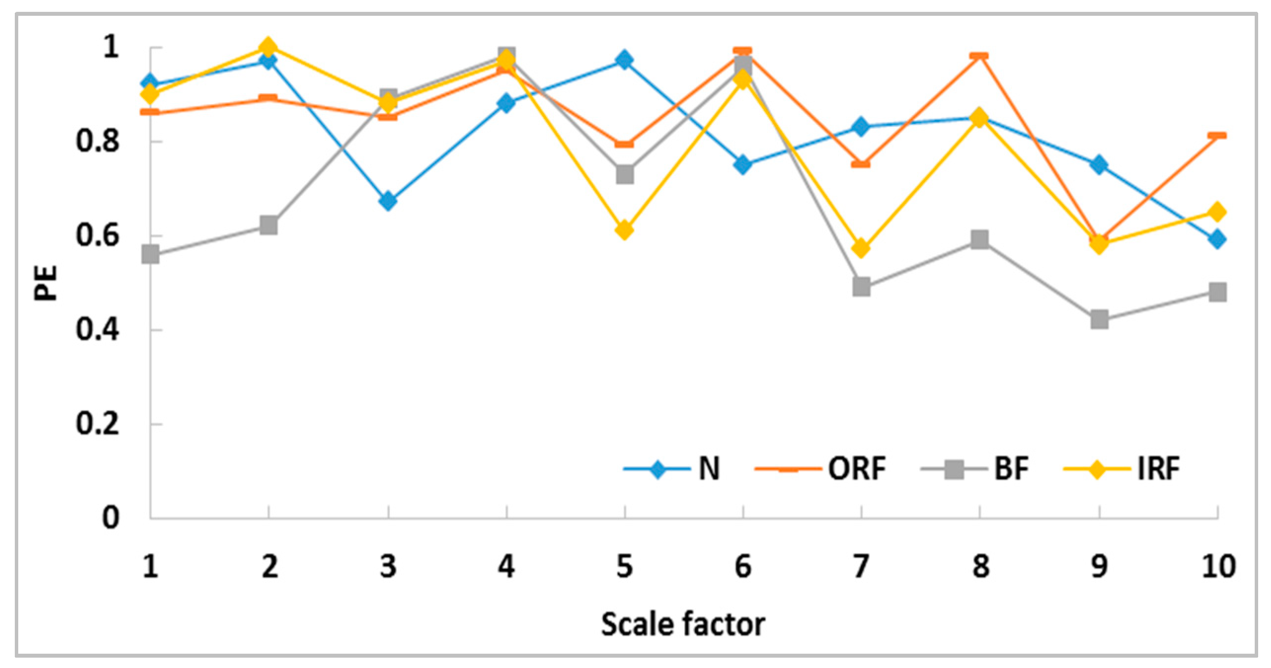
also plays an important role in feature extraction performance. The maximum scale factor 20 is selected for analysis, and the MPE curves of four types of samples are obtained as shown in 
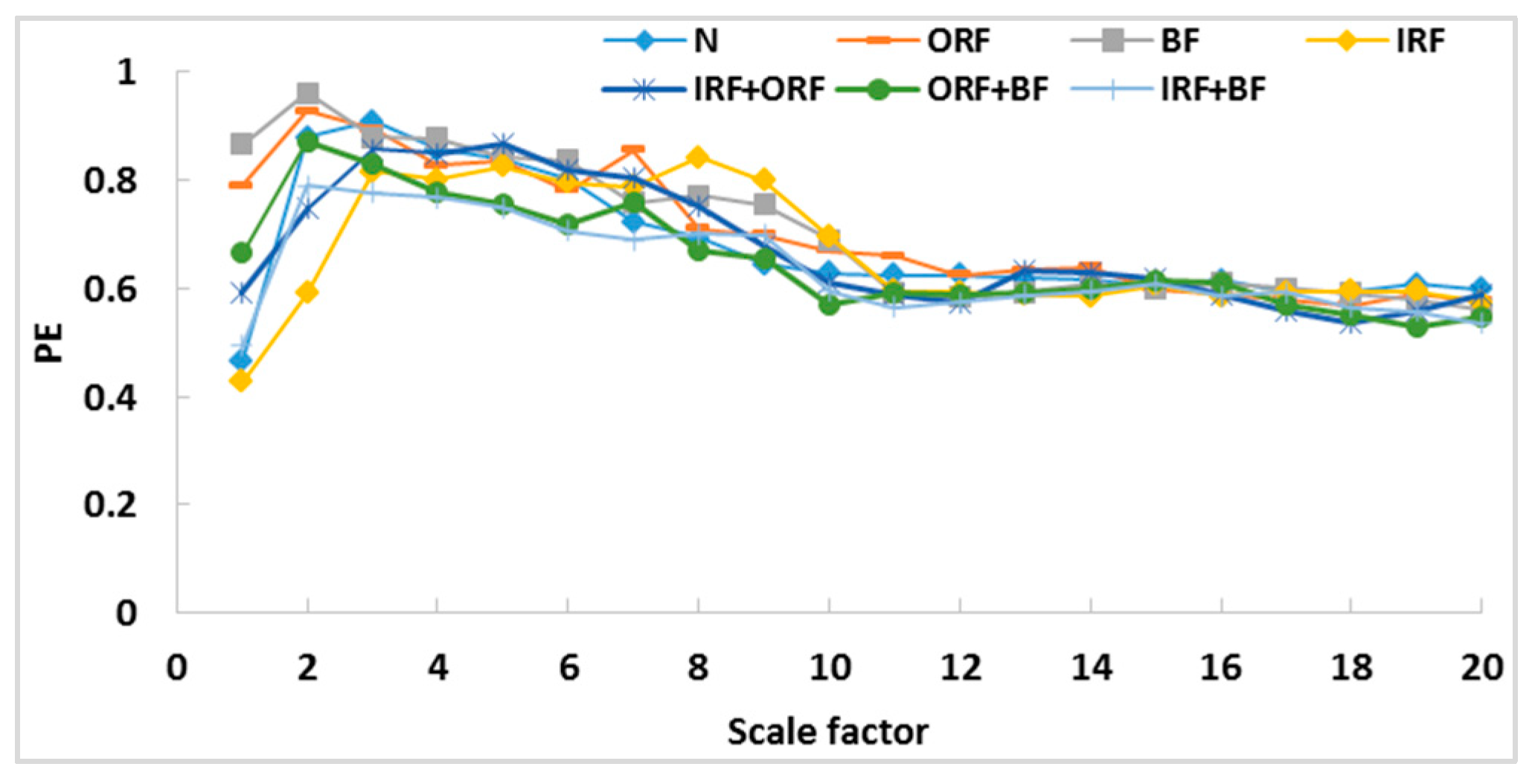
Figure 10. It can be seen that the MPE values increase first and then decrease with the increase of scale factor. At the same time, when scale factor is greater than 10, the trend of the MPE curves of different types tend to converge, which indicates that the complexity of different vibration signals tends to decrease at the same rate. This means that when the scale factor is greater than 10, it has little significance for PE to describe the complexity of the signal. As such, the scale factor was selected as 10.
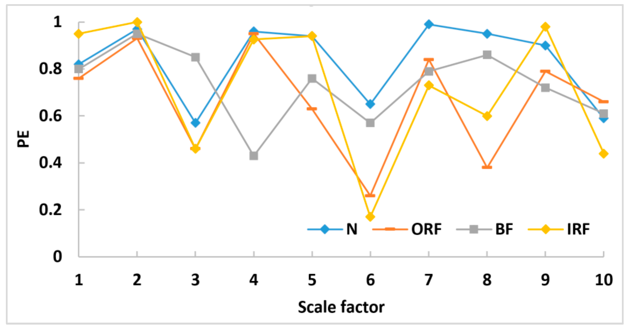
Figure 11 shows the MPE of the raw vibration signals in the four health conditions. The PE of the vibration signals with different health conditions has similar fluctuation intervals, and the intensity of fluctuation is also similar. Simultaneously, there are overlaps and intersections in the PE fluctuation range. Figure 12 and Figure 13 show the MPE of IMF1 and IMF3 for the four health conditions, respectively. The fluctuation intensity in IMF1 and IMF3 both vary greatly compared with that shown in Figure 11, and the MPE of IMF3 varies more than that of IMF1. In other words, the MPE features of IMF3 are more separable than those of IMF1 and those of the raw signal. However, the fluctuation intervals of PE still overlap. Therefore, it is not easy to directly distinguish faults with MPE parameters.
As the raw signal contains a great deal of useful information, the MPE of the raw signal was considered and fused with the IMF permutation entropy to enrich the information of the extracted feature vector. According to the training samples (N, ORF, BF, and IRF), the MPE of the selected IMFs and the raw signals were extracted. The MPE of the raw signal was recorded as MPEi, which is a 10-dimensional vector. The MPE of the first five-order IMFs was recorded as MPEj. Therefore, the final feature vector V is obtained as follows:
V = { M P E i , M P E j 1 , M P E j 2 , M P E j 3 , M P E j 4 , M P E j 5 }
The dimension of the feature vector V is 60. Through the above feature extraction method, the obtained feature vector considers the correlation of the IMFs and the raw signals themselves. It also takes advantage of MPE to characterize weak fault signals, which is beneficial in terms of establishing more abundant and comprehensive feature extraction. According to the above method, the feature vectors of all experimental samples were extracted. The MPE feature vector was then used as for input in the SSDAE network for training and testing.

3.1.4. Validation Results

As mentioned in Section 2.4.2., the proposed SSDAE contains two hidden layers. The neuron numbers of the first and second hidden layers were set to 100 and 60, respectively. The number of output layer neurons was four, which was determined by the number of bearing health conditions. The activation function was sigmoid, and the learning rates of the two hidden layers and the softmax layer were 0.1, 0.1, and 0.2, respectively. The sparsity parameter was 0.15, and the corruption level was 0.3. The detailed parameters of the SSDAE are listed in Table 3.
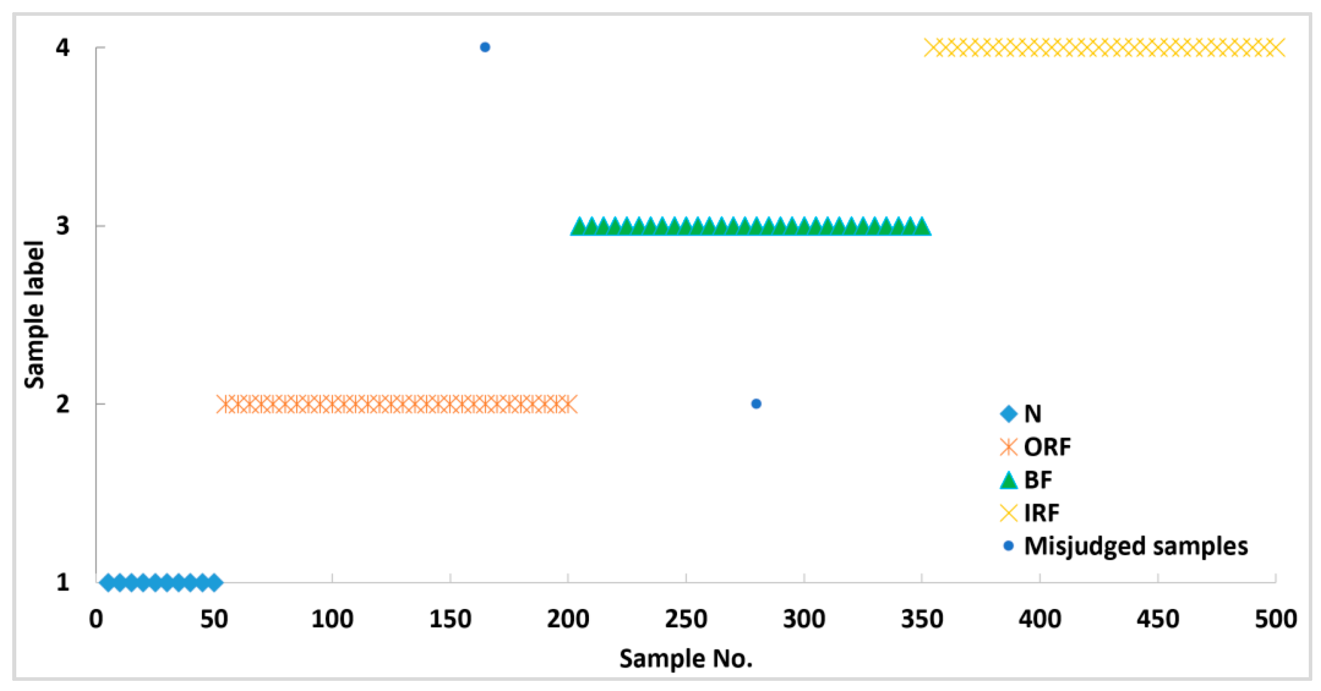
The extracted feature vector was divided into training and testing data. The former was used to train the constructed network, and the latter was used to validate the performance of the diagnosis model. Four tests were carried out, with an average classification accuracy of 99.55%. One of the test classification results is shown in Figure 14. According to the classification result, 498 out of 500 test samples were identified accurately. All samples of N and IRF were identified accurately, and only two samples were misjudged: one BF sample was misjudged as an ORF, and one ORF sample was misjudged as an IRF. The classification accuracy rate was 99.6% (498/500 = 99.6%). The experimental result shows that the proposed method based on MPE and the SSDAE can effectively detect bearing faults, and the recognition and analysis effect in different working conditions is ideal.
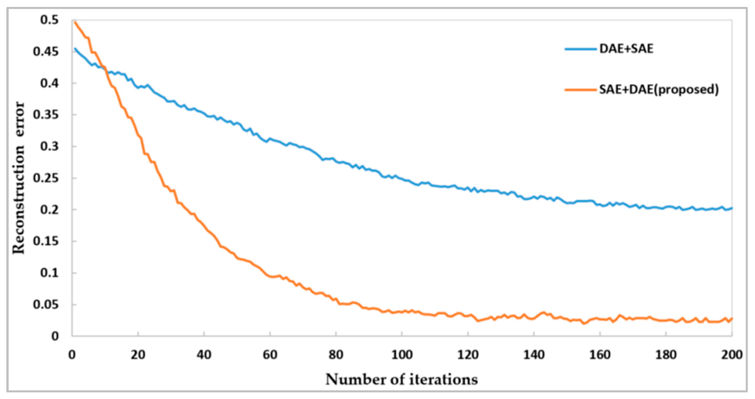
To further validate the superiority of the proposed SSDAE model structure, a comparative experiment of a different stack order, Scheme 1 (SAE + DAE), with Scheme 2 (DAE + SAE) was conducted. According to the training process of the SSDAE model, the experimental results of the two schemes were compared in the same experimental condition. Figure 15 shows that the reconstruction error of both schemes decreases as iterations increase. In Scheme 1, the reconstruction error is less than 0.05 after 100 iterations, and with the increase in iterations, the reconstruction error is stable at about 0.025. In Scheme 2, the reconstruction error is less than 0.25 after 100 iterations. With the increase in iterations, the reconstruction error decreases slowly. As the number of iterations reaches 200, the reconstruction error is still as high as 0.2. However, at the beginning of training, the reconstruction error of Scheme 1 is slightly larger than that of Scheme 2. With the increase in iterations, the reconstruction error of Scheme 1 decreases rapidly and is less than that of Scheme 2. Therefore, (the proposed) Scheme 1 is superior to Scheme 2 in terms of the real reconstruction error. One possible reason for this result is that when human visual systems process information, its mechanism is similar to sparse coding. That is, a single neuron only responds strongly to certain information. Most of the neurons in the hidden layer are suppressed, and input data are represented by sparse components. Therefore, the ability of the SAE to extract representative features is better than that of the DAE. The DAE model itself can erase the noise in the training data because the noise data is close to the test data, which can reduce the generation gap between the training and test data. Thus, in Scheme 1, the SAE is first used to extract a better feature description of the input, and the DAE is then used to enhance the robustness of feature extraction and reduce the generation gap between the training set and the testing set. Therefore, the reconstruction error of Scheme 1 was smaller. Thus, Scheme 1 would help improve the classification accuracy.
Figure 16 shows that the time required of the two schemes decreases with the increase in iterations. Each iteration time of Scheme 1 (SAE + DAE) and Scheme 2 (DAE + SAE) tends to stabilize after about 120 iterations and 80 iterations, respectively, mainly because the network has been fully trained. However, regardless of the number of iterations, Scheme 1 takes less time than Scheme 2, and each iteration time is stable at about 1s and 5s, respectively. The possible reason for this finding is that, in our experiment, the input of the SSDAE is a high-dimensional vector, and the proposed Scheme 1 starts training the SAE first, which ensures that the dimension reduction is implemented at the beginning of network training. Therefore, the network could be trained quickly from the low-dimensional vector, so each iteration time is reduced.
Some key parameters considerably influence classification accuracy or time consumption, such as the number of hidden layer neurons, the sparsity parameter, and the corruption level. Therefore, to analyze the impacts of different parameters on the diagnosis result, experiments for each parameter with different values are carried out for comparison.
The number of hidden layer neurons is important for the feature learning and classification accuracy of the SSDAE. Figure 17 shows the relationship between the number of neurons in two hidden layers with classification accuracy and time consumption. Considering dimension reduction, the number of neurons in the second hidden layer was set to be less than that in the first hidden layer, but equal or a little more than half of that in the first layer. Figure 17 shows that the classification accuracy improves gradually as the number of neurons increases. Notably, when the number of neurons in the first layer is more than 100, the classification accuracy tends to be stable, but time consumption increases linearly. Therefore, to ensure both high classification accuracy and quicker calculation speed, the number of neurons in the two hidden layers was selected as 100 and 60, respectively.
A proper sparsity parameter not only improves the feature learning ability of the network but also improves the computing efficiency. The sparsity parameter is usually a small value that is no greater than 0.5. So, the performance with sparsity parameters varying from 0.05 to 0.5 was studied in our experiments. The experimental results are shown in Figure 18. Figure 18 shows that with the increase in sparse parameter values, the classification accuracy increases gradually and then decreases gradually. When the sparsity value is greater than 0.25, the diagnosis accuracy obviously decreases. Therefore, the best diagnosis performance is obtained when the sparsity parameter is 0.15.
An excessive corruption level value may excessively remove useful information, and too small a value will affect the filtering of redundant information, thus affecting the diagnosis accuracy. The effect on classification accuracy of different corruption level values is shown in Figure 19. With the increase in the corruption level value, the classification accuracy increases gradually, and then decreases gradually. When the corruption level value is greater than 0.2 and less than 0.35, stable high classification accuracy rates are observed. When the corruption level value is greater than 0.35, the classification accuracy obviously decreases. Therefore, the best diagnosis performance is obtained when the corruption level is 0.3.
In order to know the layer-by-layer feature extraction effect of the SSDAE, the dimension reduction technology of t-SNE (t-distributed stochastic neighbor embedding) is used to reduce the dimension of each layer feature of a test set to 2 dimensions and visualize it [41]. The visualization results are shown in Figure 20. It can be seen that in the scatter plot of input data, the four states of samples are basically mixed together, and the degree of sample aggregation is poor. For each hidden layer, the features of each category are aggregated once. After the second hidden layer, each type has been basically separated. This shows that the feature distribution is greatly improved by SSDAE layer by layer feature extraction, and the ability of feature expression and distinction is stronger, thus ensuring the effective realization of subsequent state recognition and classification.
Commonly used classification models, such as the traditional stacked AE, SVM, and back-propagation neural network (BPNN), were used to validate and compare the effectiveness of the proposed SSDAE. The stacked AE has the same structure as the SSDAE. The input, hidden, and output dimensions of the BPNN were 200, 100, and 4, respectively, and sigmoid was used as an activation function. The SVM used the Gaussian kernel function. As shown in Table 4, the four methods used the same signal preprocessing (EEMD) and feature extraction (MPE) models in addition to the classification models mentioned above.
The classification results of each health condition and the total classification accuracy are shown in Table 4. The results demonstrate that the proposed method achieved the highest classification accuracy (99.6%), and the classification accuracy of each condition was also higher than the others. By comparing the first two shallow architecture methods with the last two deep learning methods, we found that, in the case of the same signal processing and feature extraction methods, methods based on the SSDAE or the stacked AE have higher classification accuracy than SVM and BPNN. This shows that deep learning method has a stronger ability in terms of feature learning and abstraction than shallow intelligent diagnosis method, especially in the case of a large number of samples with high-dimension and multi-classification issues. In addition, the SSDAE-based method achieved a higher accuracy than the stacked AE-based method, which proves that the proposed SSDAE outperforms the traditional stacked AE in extracting more representative features.
To further verify the effectiveness of the proposed feature extraction method, wavelet packet-empirical mode decomposition (WP-EMD) [42], variational mode decomposition and permutation entropy (VMD-PE) [43], and improved empirical mode decomposition energy entropy (EMDEE) [44] were considered for comparison. The features extracted by the above methods were input into the SSDAE for classification, and the classification accuracies are shown in Table 5. The proposed method achieved the highest total classification accuracy and performed better in most health conditions. Through the comparison, we observed that the feature extraction methods based on PE have higher classification accuracy than the EMD-based methods. This shows that MPE could effectively characterize and extract the volatility characteristics of different signals and mine the representative features for further diagnosis.

3.2. Experiment 2: The Laboratory Measurement Bearing Dataset

3.2.1. Experimental Data

The rotor-bearing experimental system is mainly composed of speed regulating motor, gearbox, rotating shaft, turntable, and test bearing and corresponding test system. Its structure is shown in Figure 21. During the test, the motor drives the tested bearing to rotate through the gearbox, and the motor is controlled by the frequency converter to stabilize the speed of the tested bearing in a certain range. The accelerometer is a B&K4508 vibration sensor with sensitivity of 9.782 mV/g and frequency range of 0.1-8 kHz. The data acquisition card is NIUSB-9234 with four-channel C-series dynamic signal acquisition module with USB interface.
The bearing tested on the rotor-bearing test bench is HRB6304 rolling bearing, and its parameters are shown in Table 6. Vibration signals are collected by a vibration sensor installed in the vertical direction of the bearing seat. Speed control motor speed is 2000r/min, and the sampling frequency is set to 10 KHz. The experiment simulates six different fault types shown in Figure 22, including three single point faults and three compound faults. The single point faults are IRF, ORF and BF, and the compound faults are IRF + ORF, IRF + BF, ORF + BF. The fault diameter is 0.5334 mm and the fault depth is 2.1 mm. Through the test, 1050 samples of different bearing states are obtained, each sample length is 2048 points, and the specific conditions of the seven kinds of samples are shown in Table 7.

3.2.2. Spectral Characteristic Analysis and IMFs Screening

The same as Experiment 1, fault characteristic frequencies of each part can be calculated [41]. The characteristic frequencies of IRF, ORF and BF are f I = 147.63 Hz, f O = 85.47 Hz and f B = 62.43 Hz, respectively. The time domain waveform of seven different conditions and their spectrogram are shown in Figure 23. By observing the main characteristic frequencies in the spectrum of various kinds of state signals, we find that there exists a high frequency and high amplitude component of about 3200 Hz in each kind of state signal. At the same time, in ORF, BF, IRF+ORF, IRF+BF and ORF+BF, there is a frequency component with a high frequency and relatively high amplitude of about 4800 Hz. Meanwhile, although the frequency doubling of fault characteristic frequencies can be seen under some components, there are many interference components, and the spectrum peaks of fault characteristic frequencies and their harmonics are not prominent enough. This means that there are many interference frequency components in the measured signal.
Figure 24 shows IMFs of an IRF+BF signal sample. We find it difficult to select IMFs accurately through the time-domain waveform. As shown in Figure 25, (a) is spectrogram of the raw sample and (b) are spectrograms of its eight-order IMFs. It is easy to find out from the spectrum of each IMF component that IMF1 to IMF5 contain main frequency components of the raw signal from high frequency to low frequency, respectively, and IMF6–IMF8 may be low-frequency false components. So, the first five-order IMFs were selected in Experiment 2.

3.2.3. Influence of Scale Factor Variation on MPE

The appropriate scale factor range was also analyzed in Experiment 2. The MPE curves of the seven bearing health conditions are obtained with the maximum scale factor selected as 20. As shown in Figure 26, when the scale factor is less than 10, the MPE curve of each state signal fluctuates greatly. Whereas when scale factor is greater than 10, the trend of the MPE curves of different bearing states tend to converge. This means that when scale factor is greater than 10, it has little significance for PE to describe the complexity of the signal. As such, the scale factor was also selected as 10 in Experiment 2. As in Experiment 1, with the selected parameters, MPE of the raw signal and the first five-order IMFs of each signal were calculated and fused, so dimension of the input feature vector is 60. And then MPE of all the experimental samples were extracted and used as input into the SSDAE network for training and testing.

3.2.4. Validation Results

The most parameters of the proposed SSDAE in Experiment 2 are the same as that in Experiment 1, and the number of input and output layer neurons are 60 and 7, which is determined by the dimension of the input and the number of bearing health conditions. The extracted feature vector was divided into training and testing datasets, and was put into the SSDAE model for health condition diagnosis. The average accuracy of four tests is 97.98%. Figure 27 presents the confusion matrix of the third classification results using the proposed method (classification accuracy 1033/1050 = 98.38%). The result of Experiment 2 also shows that the proposed method based on MPE and SSDAE can effectively identity bearing faults.
A comparative experiment of different stack order, Scheme 1 (SAE + DAE), with Scheme 2 (DAE + SAE) was also conducted in Experiment 2, to validate the superiority of the proposed SSDAE structure. And the experimental results were compared in the same experimental condition with Experiment 1. The test result of Scheme 1 and Scheme 2 under different iterations is shown in Figure 28. It can be seen that, as the number of iterations increases, the reconstruction error of scheme 1 decreases more quickly than that of scheme 2, and is always much smaller than that of scheme 2. Consistent with the result of Experiment 1, the result of Experiment 2 also indicates that Scheme 1 is effective in diagnosis of bearing vibration signals and it causes almost no loss of input information.
In order to verify the effectiveness of the proposed method, the stacked AE, AE, SVM, and BPNN were also used for comparison. The network structure and parameters settings of each comparison method are the same as those in Experiment 1. In order to avoid the impact of contingency, each diagnostic method has been run four times. The detailed testing accuracy of each method under four tests is shown in Figure 29. The first three methods are applied with the inputs that are preprocessing by EEMD and MPE, whereas the inputs of the remaining methods are all raw time-domain signals. Specific diagnostic accuracy and average accuracy are shown in Table 8.
As illustrated by the figure and the table, the proposed method not only has higher average fault recognition rate, but also has better diagnosis stability than other methods. We find that methods based on signal processing (EEMD) and feature extraction (MPE) have higher classification accuracy than those without any processing. This shows that the proposed feature extraction method (EEMD+MPE) could effectively extract the volatility characteristics of different signals. We also observe that with the same signal processing and feature extraction method, methods based on SSDAE or stacked AE have higher classification accuracy than those based on AE, SVM and BPNN. It shows that deep learning method has a stronger ability in terms of feature learning and abstraction than shallow intelligent diagnosis method, especially in the case of large number samples and multi-classification issues. In addition, the SSDAE-based method achieved a higher accuracy than the stacked AE-based method, which proves that the proposed SSDAE is more effective in diagnosis performance.

4. Conclusions and Future Work

Given the non-linearity and non-stationarity of bearing vibration signals, a novel diagnosis method based on SSDAE is proposed in this paper. EEMD is used for adaptive multi-scale decomposition of the vibration signal to obtain the stable component. MPE, which can effectively characterize the working characteristics of bearings in different health conditions, is used for the representative feature extraction. The proposed SSDAE was used for further feature learning and health condition classification. CWRU bearing dataset containing four health conditions with three fault severities, and the laboratory measurement bearing dataset containing seven health conditions with single fault and compound fault were used to validate the proposed method. And for the two bearing dataset diagnosis, the average classification accuracy was as high as 99.55% and 97.98%, respectively. The proposed SSDAE stack structure was compared with other stack form, and it shows that the proposed structure is superior in terms of both reconstruction error and iteration time. The influence of several key parameters on diagnosis accuracy was optimized through experiments. The proposed method was compared with the comparable methods, and results demonstrated that our method is more effective.
In the future, information about more bearing fault types needs to be collected and examined to enrich the fault database. For feature extraction, we only considered MPE method. MPE is based on the comparison between adjacent data, and extracts feature parameters reflecting signal randomness and dynamic mutation. Because it does not consider the data itself, it may ignore some information of the data itself. Hence, more efficient feature extraction methods could be developed for feature fusion to improve the classification accuracy. Generally speaking, most of the current fault detection methods are to predict the faults that have occurred and verify the effectiveness of the algorithm. However, the ultimate engineering application of fault diagnosis is to detect and predict the current faults. Therefore, online diagnosis of early health prediction on the basis of our research is worth studying.

Author Contributions

J.D. and J.T. were responsible for the overall work and proposed the idea and experiments in the paper. F.S. performed some of the experiments and contributed to many effective discussions regarding both ideas and paper writing. S.H. provided many useful suggestions and performed some of the experiments for the paper. Y.W. made many useful suggestions and comments for the paper.

Funding

This research was funded by the National Natural Science Foundation of China (Grant nos.51705531) and the Jiangsu Provincial Natural Science Foundation of China (Grant no. BK20150724).

Conflicts of Interest

The authors declare no conflict of interest.

References

  1. Cui, L.; Wu, N.; Ma, C. Quantitative fault analysis of roller bearings based on a novel matching pursuit method with a new step-impulse dictionary. Mech. Syst. Signal Process. 2016, 68, 1. [Google Scholar] [CrossRef]
  2. Liao, M.F.; Ma, Z.G.; Liu, Y.Q. Fault characteristics and diagnosis method of inter shaft bearing in aero-engine. J. Aerosp. Power 2013, 28, 2752–2758. [Google Scholar]
  3. Liu, Y.; Zhang, J.; Ma, L. A fault diagnosis approach for diesel engines based on self-adaptive WVD, improved FCBF and PECOC-RVM. Neurocomputing 2016, 177, 600–611. [Google Scholar] [CrossRef]
  4. Zarei, J.; Poshtan, J. Bearing fault detection using wavelet packet transform of induction motor stator current. Tribol. Int. 2007, 40, 763–769. [Google Scholar] [CrossRef]
  5. Prabhakar, S.; Mohanty, A.R.; Sekhar, A.S. Application of discrete wavelet transform for detection of ball bearing race faults. Tribol. Int. 2002, 35, 793–800. [Google Scholar] [CrossRef]
  6. Kankar, P.K.; Sharma, S.C.; Harsha, S.P. Rolling element bearing fault diagnosis using wavelet transform. Neurocomputing 2011, 74, 1638–1645. [Google Scholar] [CrossRef]
  7. Huang, N.E.; Zheng, S.; Long, S.R.; Wu, M.C.; Shih, H.H.; Zheng, Q.; Yen, N.C.; Chi, C.T.; Liu, H.H. The empirical mode decomposition and the Hilbert spectrum for nonlinear and non-stationary time series analysis. Proc. Math. Phys. Eng. Sci. 1998, 454, 903–995. [Google Scholar] [CrossRef]
  8. Chen, X.H.; Cheng, G.; Shan, X.L.; Hu, X.; Guo, Q.; Liu, H.G. Research of weak fault feature information extraction of planetary gear based on ensemble empirical mode decomposition and adaptive stochastic resonance. Measurement 2015, 73, 55–67. [Google Scholar] [CrossRef]
  9. Wu, Z.H.; Huang, N.E. Ensemble empirical mode decomposition: A noise assisted data analysis method. Adv. Adapt. Data Anal. 2009, 1, 1–41. [Google Scholar] [CrossRef]
  10. Lei, Y.; Li, N.; Lin, J.; Wang, S. Fault Diagnosis of Rotating Machinery Based on an Adaptive Ensemble Empirical Mode Decomposition. Sensors 2013, 13, 16950–16964. [Google Scholar] [CrossRef] [Green Version]
  11. Bandt, C.; Pompe, B. Permutation entropy: A natural complexity measure for time series. Phys. Rev. Lett. 2002, 88, 174102. [Google Scholar] [CrossRef] [PubMed]
  12. Olofsen, E.; Sleigh, J.W.; Dahan, A. Permutation entropy of the electroencephalogram: A measure of anaesthetic drug effect. Br. J. Anaesth. 2008, 101, 810–821. [Google Scholar] [CrossRef]
  13. Wu, S.D.; Wu, P.H.; Wu, C.W.; Ding, J.J.; Wang, C.C. Bearing Fault Diagnosis Based on Multiscale Permutation Entropy and Support Vector Machine. Mol. Divers. Preserv. Int. 2012, 14, 1343–1356. [Google Scholar] [CrossRef] [Green Version]
  14. Arenas, A.; Aziz, B.; Bicarregui, J. An Event-B approach to data sharing agreements. In Integrated Formal Methods-IFM; Furia, C.A., Winter, K., Eds.; Springer: Berlin, Germany, 2010. [Google Scholar]
  15. D’addona, D.M.; Ullah, A.M.M.S.; Matarazzo, D. Tool-wear prediction and pattern-recognition using artificial neural network and DNA-based computing. J. Intell. Manuf. 2017, 28, 1–17. [Google Scholar] [CrossRef]
  16. Yu, H.; Khan, F.; Garaniya, V.; Ahmad, A. Self-Organizing Map Based Fault Diagnosis Technique for Non-Gaussian Processes. Ind. Eng. Chem. Res. 2014, 53, 8831–8843. [Google Scholar] [CrossRef]
  17. Wang, Y.; Zhang, N.; Li, J.; Wang, G. Application of wavelet packet in motor fault diagnosis. J. Changchun Univ. Technol. 2013, 34, 387–391. [Google Scholar]
  18. Liu, Z.; Chen, X.; He, Z.; Shen, Z. LMD Method and Multi-Class RWSVM of Fault Diagnosis for Rotating Machinery Using Condition Monitoring Information. Sensors 2013, 13, 8679–8694. [Google Scholar] [CrossRef] [Green Version]
  19. Xue, Y.; Li, Z.; Wang, B.; Zhao, Z.; Li, F. Nonlinear feature selection using Gaussian kernel SVM-RFE for fault diagnosis. Appl. Intell. 2018, 1, 1–26. [Google Scholar] [CrossRef]
  20. Zhang, X.; Zhang, Q.; Qin, X.; Sun, Y. Rolling bearing fault diagnosis based on ITD Lempel-Ziv complexity and PSO-SVM. J. Vib. Shock 2016, 35, 102–107. [Google Scholar]
  21. Liang, S.; Chen, Y.; Liang, H.; Li, X. Sparse Representation and SVM Diagnosis Method for Inter-Turn Short-Circuit Fault in PMSM. Appl. Sci. 2019, 9, 224. [Google Scholar] [CrossRef]
  22. Vincent, P.; Larochelle, H.; Bengio, Y.; Manzagol, P.A. Extracting and composing robust features with denoising autoencoders. In Proceedings of the International Conference on Machine Learning, Vancouver, BC, Canada, 20–24 June 2008. [Google Scholar]
  23. Vincent, P.; Larochelle, H.; Lajoie, I.; Bengio, Y.; Manzagol, P.A. Stacked denoising autoencoders: Learning useful representations in a deep network with a local denoising criterion. J. Mach. Learn. Res. 2010, 11, 3371–3408. [Google Scholar]
  24. Hinton, G.E.; Osindero, S.; Teh, Y.W. A fast learning algorithm for deep belief nets. Neural Comput. 2006, 18, 1527–1554. [Google Scholar] [CrossRef] [PubMed]
  25. Krizhevsky, A.; Sutskever, I.; Hinton, G.E. ImageNet classification with deep convolutional neural networks. In Proceedings of the International Conference on Neural Information Processing Systems, Lake Tahoe, NV, USA, 3–6 December 2012; pp. 1097–1105. [Google Scholar]
  26. Chen, Z.Q.; Li, C.; Sanchez, R.V. Gearbox fault identification and classification with convolutional neural networks. Shock Vib. 2015, 18, 1155–1164. [Google Scholar] [CrossRef]
  27. Gan, M.; Wang, C.; Zhu, C.A. Construction of hierarchical diagnosis network based on deep learning and its application in the fault pattern recognition of rolling element bearings. Mech. Syst. Signal Process. 2016, 72–73, 92–104. [Google Scholar] [CrossRef]
  28. Baraldi, P.; Di Maio, F.; Genini, D.; Zio, E. Comparison of Data-Driven Reconstruction Methods For Fault Detection. IEEE Trans. Reliab. 2015, 64, 852–860. [Google Scholar] [CrossRef] [Green Version]
  29. Bengio, Y. Learning Deep Architectures for AI. Found. Trends Mach. Learn. 2009, 2, 1–127. [Google Scholar] [CrossRef]
  30. Jia, F.; Lei, Y.; Lin, J.; Zhou, X. Deep neural networks: A promising tool for fault characteristic mining and intelligent diagnosis of rotating machinery with massive data. Mech. Syst. Signal Process. 2016, 72, 303–315. [Google Scholar] [CrossRef]
  31. Xia, M.; Li, T.; Liu, L.; Xu, L.; Silva, C.W.D. An Intelligent Fault Diagnosis Approach with Unsupervised Feature Learning by Stacked Denoising Autoencoder. IET Sci. Meas. Technol. 2017, 11, 687–695. [Google Scholar] [CrossRef]
  32. Tan, J.; Lu, W.; An, J. Fault diagnosis method study in roller bearing based on wavelet transform and stacked auto-encoder. In Proceedings of the IEEE Control & Decision Conference, Osaka, Japan, 15–18 December 2015. [Google Scholar]
  33. Sohaib, M.; Kim, C.H.; Kim, J.M. A Hybrid Feature Model and Deep-Learning-Based Bearing Fault Diagnosis. Sensors 2017, 17, 2876. [Google Scholar] [CrossRef]
  34. Meng, L.; Ding, S.; Zhang, N. Research of stacked denoising sparse autoencoder. Neural Comput. Appl. 2016, 30, 2083–2100. [Google Scholar] [CrossRef]
  35. Huang, N.E.; Wu, M.L.C.; Long, S.R. A confidence limit for the empirical mode decomposition and Hilbert spectral analysis. Proc. R. Soc. Lond. Ser. A Math. Phys. Eng. Sci. 2003, 459, 2317–2345. [Google Scholar] [CrossRef]
  36. Rilling, G.; Flandrin, P. One or two frequencies? The empirical mode decomposition answers. IEEE Trans. Signal Process. 2007, 56, 85–95. [Google Scholar] [CrossRef]
  37. Zheng, J.D.; Cheng, J.S.; Yang, Y. Multi-scale permutation entropy and its applications to rolling bearing fault diagnosis. China Mech. Eng. 2013, 24, 2641–2646. [Google Scholar]
  38. Bengio, S.; Pereira, F.; Singer, Y.; Strelow, D. Group sparse coding. In Proceedings of the International Conference on Neural Information Processing Systems, Vancouver, BC, Canada, 7–10 December 2009. [Google Scholar]
  39. Smith, W.A.; Randall, R.B. Rolling element bearing diagnostics using the Case Western Reserve University data: A benchmark study. Mech. Syst. Signal Process. 2015, 64–65, 100–131. [Google Scholar] [CrossRef]
  40. Wardle, F.P. Vibration forces produced by waviness of the rolling surfaces of thrust loaded ball bearings. Part2, Experimental validation. Proc. Inst. Mech. Eng. Part C J. Mech. Eng. Sci. 1988, 202, 313–319. [Google Scholar] [CrossRef]
  41. Maaten, L.V.D.; Hinton, G. Visualizing data using t-SNE. J. Mach. Learn. Res. 2008, 9, 2579–2605. [Google Scholar]
  42. Hong, S.; Zhou, Z.; Zio, E.; Hong, K. Condition assessment for the performance degradation of bearing based on a combinatorial feature extraction method. Dig. Signal Process. 2014, 27, 159–166. [Google Scholar] [CrossRef]
  43. Tang, G.; Wang, X.; He, Y.; Liu, S. Rolling bearing fault diagnosis based on variational mode decomposition and permutation entropy. In Proceedings of the 13th International Conference on Ubiquitous Robots and Ambient Intelligence (URAI), Xi’an, China, 19–22 August 2016. [Google Scholar]
  44. Huang, J.; Hu, X.; Xin, G. An intelligent fault diagnosis method of high voltage circuit breaker based on improved EMD energy entropy and multi-class support vector machine. Electr. Power Syst. Res. 2011, 81, 400–407. [Google Scholar] [CrossRef]
Figure 1. Flow chart of the proposed diagnosis method.
Applsci 09 02743 g001
Figure 2. Permutation entropy (PE) of Gaussian white noise in different embedding dimensions.
Applsci 09 02743 g002
Figure 3. PE of Gauss white noise with different time delays.
Applsci 09 02743 g003
Figure 4. Structure of autoencoder (AE).
Applsci 09 02743 g004
Figure 5. The construction and training of the stacked sparse denoising autoencoder (SSDAE). (a) the shallow sparse autoencoder (SAE), (b) the shallow denoising autoencoder (DAE), (c) the constructed SSDAE network, and (d) the proposed supervised learning SSDAE network.
Applsci 09 02743 g005
Figure 6. Bearing test ring. A = fan end bearing; B = electronic motor; C = drive end bearing; D = torque transducer; E = dynamometer.
Applsci 09 02743 g006
Figure 7. Time domain waveform and spectrogram of the four health conditions. (a) Normal condition (N); (b) Outer race fault (ORF); (c) Ball fault (BF); (d) Inter race fault (IRF).
Applsci 09 02743 g007
Figure 8. Eight-order IMFs of a BF signal decomposed by ensemble empirical mode decomposition (EEMD).
Applsci 09 02743 g008
Figure 9. Spectrogram of a BF signal and its IMFss. (a) Spectrogram of a BF signal sample; (b) Spectrogram of the eight-order IMFs.
Applsci 09 02743 g009
Figure 10. Multiscale permutation entropy (MPE) of bearing signals for four health conditions with different scale factor.
Applsci 09 02743 g010
Figure 11. MPE of the raw vibration signals for four health conditions.
Applsci 09 02743 g011
Figure 12. MPE of intrinsic mode function 1 (IMF1) for four health conditions.
Applsci 09 02743 g012
Figure 13. MPE of IMF3 for four health conditions.
Applsci 09 02743 g013
Figure 14. Classification result of the proposed method for bearing dataset.
Applsci 09 02743 g014
Figure 15. Reconstruction error of the two schemes.
Applsci 09 02743 g015
Figure 16. The contrast chart of the iteration time between the two schemes.
Applsci 09 02743 g016
Figure 17. Effect of the number of neurons in two hidden layers.
Applsci 09 02743 g017
Figure 18. Classification accuracy of the proposed method with different sparsity parameters.
Applsci 09 02743 g018
Figure 19. Classification accuracy of the proposed method with different corruption levels.
Applsci 09 02743 g019
Figure 20. Visualization results of each layer.
Applsci 09 02743 g020
Figure 21. Rotor-bearing experimental system.
Applsci 09 02743 g021
Figure 22. Bearing single point fault and compound fault.
Applsci 09 02743 g022
Figure 23. Time domain waveform and spectrogram of different health conditions in Experiment 2. (a) Normal condition (N); (b) Outer race fault (ORF); (c) Ball fault (BF); (d) Inter race fault (IRF); (e) IRF+ORF; (f) IRF+BF; (g) ORF+BF.
Applsci 09 02743 g023aApplsci 09 02743 g023b
Figure 24. Eight-order IMFs of an IRF+BF signal decomposed by EEMD.
Applsci 09 02743 g024
Figure 25. Spectrogram of an IRF+BF and its IMF Components. (a) Spectrogram of an IRF+BF signal sample; (b) Spectrogram of the eight-order IMFs.
Applsci 09 02743 g025aApplsci 09 02743 g025b
Figure 26. MPE of seven health conditions with different scale factors in Experiment 2.
Applsci 09 02743 g026
Figure 27. Confusion matrix diagram of the third test result using the proposed method.
Applsci 09 02743 g027
Figure 28. Reconstruction error of the two schemes in Experiment 2.
Applsci 09 02743 g028
Figure 29. Diagnosis results of the four tests.
Applsci 09 02743 g029
Table 1. The employed drive end (DE) bearing parameters (mm) in Experiment 1.
TypeOutside Diameter Inside DiameterThicknessBall DiameterPitch DiameterNumber of Balls
6205-2RS
JEM SKF
5225157.94399
Table 2. Training and testing samples of the bearing dataset in Experiment 1.
Fault TypeFault Diameter
(mm)
Training SamplesTesting SamplesSample LengthSample Label
N01005020481
ORF0.18/0.36/0.54100/100/10050/50/502
BF0.18/0.36/0.54100/100/10050/50/503
IRF0.18/0.36/0.54100/100/10050/50/504
Table 3. The proposed stacked sparse denoising autoencoder (SSDAE) network parameters.
No. of Hidden LayersNo. of Input Layer NeuronsNo. of Hidden Layer NeuronsNo. of Output Layer NeuronsActivation Function
260100,604sigmoid
Epoch NumberCorruption LevelLearning RateSparsity ParameterSparsity Penalty Term
1000.30.1,0.1,0.20.153
Table 4. Classification accuracy (%) using different classification models.
MethodsNORFBFIRFTotal
EEMD + MPE + SSDAE (proposed)10099.3399.3310099.60
EEMD + MPE + Stacked AE98.0098.6798.0096.6797.80
EEMD + MPE + SVM10095.3392.6790.0093.40
EEMD + MPE + BPNN90.0092.6790.6787.3390.20
Table 5. Classification accuracy (%) using different feature extraction methods.
MethodsNORFBFIRFTotal
EEMD-MPE (proposed)10099.3399.3310099.60
VMD-PE10010099.3398.6799.20
WP-EMD98.0098.0098.6799.3398.60
EMDEE94.0098.6798.0097.3397.60
Table 6. HRB6304 bearing parameters (mm).
ParameterInner Ring DiameterOuter Ring DiameterPitch DiameterBall DiameterNumber of Balls
Value2052369.67
Table 7. Samples of the bearing in Experiment 2.
Fault TypeTraining SamplesTest SamplesSample LengthSample Label
N30015020481
ORF3001502
BF3001503
IRF3001504
IRF+ORF3001505
IRF+BF3001506
ORF+BF3001507
Table 8. Average classification accuracy (%) of the proposed method and the comparative methods.
MethodsClassification Accuracy (%)
Test 1Test 2Test 3Test 4Average Accuracy
EEMD + MPE + SSDAE97.998.1998.3897.4397.98
EEMD + MPE + Stacked AE96.8695.996.1994.4895.86
EEMD + MPE + SVM92.4793.3388.4891.4391.43
Stacked AE90.0989.6289.2490.4788.07
AE82.9586.7684.9583.986.43
SVM66.6763.862.9563.2464.17
BPNN37.2433.7138.5735.3336.21

