Memory-Enhanced Dynamic Multi-Objective Evolutionary Algorithm Based on L_p Decomposition

Abstract

Decomposition-based multi-objective evolutionary algorithms provide a good framework for static multi-objective optimization. Nevertheless, there are few studies on their use in dynamic optimization. To solve dynamic multi-objective optimization problems, this paper integrates the framework into dynamic multi-objective optimization and proposes a memory-enhanced dynamic multi-objective evolutionary algorithm based on $L_p$ decomposition (denoted by dMOEA/D-$L_p$). Specifically, dMOEA/D-$L_p$ decomposes a dynamic multi-objective optimization problem into a number of dynamic scalar optimization subproblems and coevolves them simultaneously, where the $L_p$ decomposition method is adopted for decomposition. Meanwhile, a subproblem-based bunchy memory scheme that stores good solutions from old environments and reuses them as necessary is designed to respond to environmental change. Experimental results verify the effectiveness of the $L_p$ decomposition method in dynamic multi-objective optimization. Moreover, the proposed dMOEA/D-$L_p$ achieves better performance than other popular memory-enhanced dynamic multi-objective optimization algorithms.

1. Introduction

In the real world, many problems can be described as multi-objective optimization problems (MOPs), where multiple objectives often conflict with each other. Each objective has to compromise in optimization, and finally generate a set of balanced solutions, called the Pareto optimal set (POS) [1], which is provided to decision makers. Evolutionary multi-objective optimization, referred to EMO, focuses on using evolutionary algorithms for MOPs [2]. Its research has become a hot topic in the field of evolutionary computation. MOPs can be further divided into static and dynamic multi-objective problems (DMOPs). In the dynamic environment, the objective function, constraint function, and the related parameters of DMOPs can change with time [3]. Therefore, a dynamic evolutionary multi-objective optimization algorithm (DEMOA) must be able to automatically detect and respond to new changes with fast convergence, and track the time-varying POS in a timely fashion. As a result, this study brings new challenges to EMO [4]. In the past ten years, some researchers have had strong interest in dynamic EMO (DEMO) [5,6]. Based on genetic algorithms, artificial immune algorithms [7,8], particle swarm optimization algorithms [9,10], co-evolutionary algorithms [11], membrane computing [12,13], and other natural computing methods, they designed the corresponding DEMOAs [14]. DEMOAs have been preliminarily used in intelligent service [15], industrial design [16], engineering management [17], scheduling control and optimization [18], and other fields. For their further researches have important theoretical significance and practical applied value.

How to make a rapid response to a new environment using an obtained optimal solution is very important in the design of a DEMOA. Memory methods can reuse the previous optimal solutions by remembering to help the algorithm make a good response to the new changes. There are some dynamic single objective evolutionary algorithms with memory methods to enhance the dynamic tracking performance [19,20]. So far, however, few memory methods are used in DEMOAs. In 2007, the famous dynamic non-dominated sorting genetic algorithm II (DNSGA-II) [16] was proposed by Deb et al., which was based on NSGA-II [21]. In 2009, Goh et al. proposed a collaborative multi-objective evolutionary algorithm for dynamic competition cooperation, named the dynamic competition-cooperation co-evolutionary algorithm (dCOEA) [12]. Koo and Goh et al. proposed a dynamic multi-objective evolutionary gradient search algorithm (dMO-EGS) [22] in 2010. Shang et al. proposed an immune clonal coevolutionary algorithm for dynamic multi-objective optimization (QICCA) [7] in 2014. All these DEMOAs have tried to use memory methods to quickly respond to new changes, but the actual effects are not ideal.

In addition to rapid response and dynamic tracking, another difficulty in designing a DEMOA is that the Pareto solutions set obtained by the algorithm should has good convergence and distribution in each process of environment change. At present, most DEMOAs follow the traditional approaches of static evolutionary multi-objective optimization and use the Pareto domination and elite reserved strategies to ensure the convergence. They also use the operators of diversity maintaining to ensure the diversity of the Pareto solutions. Zhang et al. proposed a new framework called the multi-objective evolutionary algorithm based on decomposition (MOEA/D) for solving static MOPs in 2007 [23]. MOEA/D decomposes a multi-objective problem into a number of single-objective sub-problems and solves these subproblems in parallel. MOEA/D has become very popular in solving static MOPs, but fewer decomposition-based DMOEAs are researched for DMOPs. In this paper, we introduce this framework and propose a memory-enhanced dynamic multi-objective algorithm based on $L_p$ decomposition for solving DMOPs, where the $L_p$ decomposition method is presented. The proposed algorithm is abbreviated as dMOEA/D-$L_p$.

The rest of this paper is organized as follows. Section 2 introduces some related works, including the basic definitions of dynamic optimization. Section 3 introduces the background knowledge on decomposition approaches and memory methods. Section 3.4 describes the framework of our proposed algorithm: dMOEA/D-$L_p$ (memory-enhanced dynamic multi-objective algorithm based on $L_p$ decomposition). Section 4 presents experimental studies on dMOEA/D-$L_p$. Finally, Section 5 concludes.

2. Related works

2.1. Problem Description and Basic Definitions

Without loss of generality, an MOP with n decision variables and m objective functions can be described as:

$$\begin{array}{c}\left\{\begin{array}{c}\underset{x\in \mathsf{\Omega }}{min}F(x)={(f_1(x),f_2(x),\dots ,f_m(x))}^{\top },\hfill \\ \mathrm{s}.\mathrm{t}.g_i(x)\le 0,i=1,2,\dots ,s;h{}_j(x)=0,j=1,2,\dots ,q,\hfill \end{array}\right.\hfill \end{array}$$

(1)

where $x={(x_1,x_2,\dots ,x_n)}^T\in \mathsf{\Omega }\subset R^n$ is a vector of decision variables, $\mathsf{\Omega }$ is the n-dimensional decision space, and $F(x)={(f_{1,}{f}_{2,},\dots ,f_m)}^T\in \mathsf{\Lambda }\subset R^m$ is an m-dimensional vector of m objective functions. $R^m$ is called the objective space. The evaluation function $F(x):\mathsf{\Omega }\to \mathsf{\Lambda }$ defines m mapping from the decision space to the objective space. $g_i(x)\le 0(i=1,2,\dots ,s)$ are some inequality constraints, and $h_j(x)=0(j=1,2,\dots ,q)$ are some q equality constraints [24].

The time variable of t is included in DMOP. Based on a static multi-objective problem, we can make an extension naturally. It involves an n-dimensional decision variable x, m-objective functions, and the constraint conditions. The objective functions and the constraint conditions are functions of the decision variable x. The mathematical model of a DMOP is expressed as:

$$\begin{array}{c}\left\{\begin{array}{c}\underset{x\in \mathsf{\Omega }}{min}F(x,t)={(f_1(x,t),f_2(x,t),\dots ,f_m(x,t))}^{\top },\hfill \\ \mathrm{s}.\mathrm{t}.g_i(x,t)\le 0,i=1,2,\dots ,s;h{}_j(x,t)=0,j=1,2,\dots ,q,\hfill \end{array}\right.\hfill \end{array}$$

(2)

where the evaluation function $F(x,t)$, the inequality constraint function $g_i(x,t)$, and the equality constraint function $h_j(x,t)$ may change with time t.

Definition 1 (The relation of Pareto dominance).

For any two decision vectors u and v, the vector $u={(u_1,u_{2,}\dots ,u_m)}^T$ dominates vector $v={(v_1,v_{2,}\dots ,v_m)}^T$, denoted by $u\prec v$, only if: $\forall k\in \{1,2,\dots ,m\}$, ${\mathrm{u}}_k\le v_k$ and $\exists l\in \{1,2,\dots ,m\}$, $u_l<v_l$.

Definition 2 (Pareto optimal solution).

The decision vector $x\in \mathsf{\Omega }$ is the Pareto optimal solution, if and only if $\neg \exists x^{\prime }\in \mathsf{\Omega }$ satisfying $F(x^{\prime },t)\prec F(x,t)$.

Definition 3 (Pareto optimal set (POS(t))).

The Pareto optimal set (POS) is the set that consists of all Pareto optimal solutions. The POS of a DMOP is defined as POS$(t):\{x\in \mathsf{\Omega }\left|\neg \exists x^{\prime }\in \mathsf{\Omega },F(x^{\prime },t)\prec F(x,t)\right.\}$.

Definition 4 (Pareto optimal front (POF(t))).

The Pareto optimal front (POF) of a DMOP is defined as POF$(t):=\{F(x,t)\left|x\in POS(t)\right.$. The Pareto optimal front (POF) is the set of all the Pareto optimal objective vectors.

From the proposal of Farina et al. [3], there are four different types of DMOPs according to the changes affecting the Pareto optimal front and the Pareto optimal set.

• Type I: where POS(t) changes while POF(t) remains invariant.
• Type II: where both POS(t) and POF(t) change.
• Type III: where POF(t) changes while POS(t) remains invariant.
• Type IV: where both POS(t) and POF(t) remain invariant.

This classification shows the difficulty of solving DMOPs by describing the combination of changes in the Pareto set and front.

2.2. Decomposition Methods

Decomposition-based multi-objective evolutionary algorithms have become an extremely prevailing framework for multi-objective optimization. Their main idea is to decompose an MOP into a number of scalaring sub-problems and solve them in parallel, where the decomposition method plays an extremely important role. There are three commonly used decomposition methods [23]: weighted sum approach (WS) [25], Tchebycheff approach (TCH) [25] and the penalty-based boundary intersection approach (PBI) [23,26], described as follows.

• Weighted Sum (WS) approach

The DMOPs of Formula (2) are decomposed into N dynamic scalar optimization subproblems by using N different uniformly distributed weight vectors ${\lambda }^i=({\lambda }_1^i,{\lambda }_2^i,\dots ,{\lambda }_m^i)(i=1,2,\dots ,N)$, where for all $i=1,2,\dots ,N$, ${\lambda }_j^i\ge 0$ and ${\displaystyle \sum _{j=1}^m}{\lambda }_j^i=1$.

With this approach, the decomposed scalar subproblem can be described as follows:

$$\begin{array}{c}\left\{\begin{array}{c}\underset{x\in \mathsf{\Omega }}{min}{g}^{ws}(x,t\left|\lambda \right.)={\displaystyle \sum _{i=1}^m}{\lambda }_i{f}_i(x,t),\hfill \\ \mathrm{s}.\mathrm{t}.g_i(x,t)\le 0,i=1,2,\dots ,s;h_j(x,t)=0,j=1,2,\dots ,q.\hfill \end{array}\right.\hfill \end{array}$$

(3)

$x={(x_1,x_2,\dots ,x_n)}^T$ are n variables to be optimized. We can use different weight vectors to generate a set of different scalar optimization problems. $g_i(x,t)$ and $h_j(x,t)$ are s inequality and q equality constraint functions, respectively.

• Tchebycheff (TCH) approach

Referring to the standard Tchebycheff formula in the static multi-objective problem, under the condition of adding time, a dynamic Tchebycheff scalar optimization problem can be described as:

$$\begin{array}{c}\left\{\begin{array}{c}\underset{x\in \mathsf{\Omega }}{min}{g}^{tch}(F(x,t)\left|\lambda ,z^{\ast }(t)\right.)=\underset{1\le i\le m}{max}\left\{{\lambda }_i\left|f_i(x,t)-z^{\ast }(t)\right|\right\},\hfill \\ \mathrm{s}.\mathrm{t}.g_i(x,t)\le 0,i=1,2,\dots ,s;h_j(x,t)=0,j=1,2,\dots ,q,\hfill \end{array}\right.\hfill \end{array}$$

(4)

where $\lambda ={({\lambda }_1,{\lambda }_2,\dots ,{\lambda }_m)}^T$ is the same as the WS approach, t is a time variable, and $z^{\ast }(t)={(z_1^{\ast }(t),\dots ,z_m^{\ast }(t))}^T$ is a reference point. That is, for each $i=1,\dots ,m$, $z_i^{\ast }(t)=min\left\{f_i(x,t)\left|g(x,t)\le 0;h(x,t)=0;x\in \mathsf{\Omega }\right.\right\}$. For each Pareto optimal solution $x^{\ast }$ of MOPs in Formula (2), there is a corresponding weight vector $\lambda$, so that $x^{\ast }$ is the optimal solution of Formula (4). Each optimal solution of Formula (4) is also the Pareto optimal solution [23] of MOPs in Formula (2). Therefore, different Pareto optimal solutions can be obtained by changing the weight vectors. Thus, MOPs can be decomposed and transformed into multiple Tchebycheff scalar optimization subproblems with different weight vectors.

• Penalty-based boundary intersection (PBI) approach

A dynamic PBI scalar optimization problem can be described as:

$$\begin{array}{c}\left\{\begin{array}{c}\underset{x\in \mathsf{\Omega }}{min}{g}^{pbi}(x,t\left|\lambda ,z^{\ast }(t)\right.)=d_1+\theta d_2,\hfill \\ d{}_1=\frac{∥{(z^{\ast }(t)-F(x,t))}^T\lambda ∥}{∥\lambda ∥},d{}_2=∥F(x,t)-(z^{\ast }(t)-d_1\lambda )∥,\hfill \\ \mathrm{s}.\mathrm{t}.g_i(x,t)\le 0,i=1,2,\dots ,s;h_j(x,t)=0,j=1,2,\dots ,q,\hfill \end{array}\right.\hfill \end{array}$$

(5)

where $g^{pbi}(x,t\left|\lambda ,z^{\ast }(t)\right.)$ is dynamic scalar objective function. $z^{\ast }$ is the ideal reference point as defined in (4), and $\theta$ is the default penalty parameter. $F(x,t)$ is the evaluation function in Formula (2), $d_1$ and $d_2$ are two distance values [23], t is a time variable. According to previous experience [23], when using the same distributed weighted vectors, the PBI approach has a slight advantage over the TCH approach when solving MOPs with more than two objectives. However, the benefits come with the price that the penalty parameter $\theta$ needs to be adjusted properly.

2.3. Memory-Enhanced Algorithm for Environmental Change

Many practical optimization problems show periodic change approximation, such as city traffic changes [20], where the optimal solution in the new environment may return to the previously searched locations. Then, with a memory method reusing the previously searched solutions, a dynamic evolutionary algorithm will have a better tracking performance. According to how much information needs to be stored, memory methods can commonly be divided into short-term memory and medium-term memory (given the limited computing resources, long-term memory methods are rarely used). Short-term memory methods only need to remember the optimal solutions of the last changed environment. On the contrary, in medium-term memory methods, the optimal solutions of several previous environmental changes need to be remembered.

2.3.1. DEMO Algorithm with Short-Term Memory

(1)

The immune clonal coevolutionary algorithm for dynamic multi-objective optimization (QICCA) algorithm is a short-term memory approach [7].

To ensure a good convergence rate, the QICCA algorithm makes the final antibody population as the initial population of the next moment. The algorithm preserves all the best solutions in the previous change environment and has an effect of short-term memory.

(2)

DNSGA-II algorithm with short-term memory and diversity [23]

The DNSGA-II algorithm (this paper named it short-term memory and diversity introduction, or SMDI) responds to new environmental change through a short-term memory and diversity introduction operation. SMDI first retains most of the individuals in the previous generation of environmental change. It has a short-term memory effect. Then, in order to respond to new changes, it randomly initializes some other individuals in the current population to introduce a small amount of diversity to the population.

The memory methods in the above two DEMOAs are simple and easy to use, but they can only remember the optimal solutions of the last previous environmental change, and thus their memory capacity is limited. Especially when the environments change sharply, the memory effect is basically lost.

2.3.2. DEMO Algorithm with Medium-Term Memory

If an evolutionary algorithm is added to such a medium-term memory method (memory pool + store procedure + retrieve process), among them the memory pool holds the best solutions of the past. The store procedure is responsible for storing the optimal solutions in the memory pool, and the retrieval process is responsible for retrieving the optimal solutions from the memory pool and inserting them into the population of the new environment. Then, the evolutionary algorithm can reuse the optimal solutions of several previous environmental changes and have a better response to the new change. According to Branke [27], there are three important issues in the design of medium-term memory methods.

(1)

When should put the individuals deposited into the memory pool in the population?

(2)

How many individuals should be stored in the memory pool, and which individuals should be replaced to make room for the memory pool to accommodate new individuals?

(3)

Which individuals are retrieved from the memory pool and reinserted into the population?

3. Memory-Enhanced Dynamic Multi-Objective Evolutionary Algorithm Based on ${\mathit{L}}_{\mathit{p}}$ Decomposition

A memory-enhanced dynamic multi-objective evolutionary algorithm based on $L_p$ decomposition (dMOEA/D-$L_p$) is proposed in this paper. Specifically, dMOEA/D-$L_p$ decomposes a dynamic multi-objective optimization problem into a number of dynamic scalar optimization subproblems and optimizes them simultaneously, where the $L_p$ decomposition method is presented and used. Meanwhile, an improved environment detection operator is presented for dynamic environments. Additionally, a subproblem-based memory scheme that allows the evolutionary algorithm to store good solutions from old environments and reuse them as necessary is designed to respond to the environmental change. The overall framework of dMOEA/D-$L_p$ can be seen at the end of this subsection. We present the $L_p$ decomposition method in step 2 of the dMOEA/D-$L_p$. An improved environmental change detection operator and a subproblem-based bunchy memory scheme are presented in step 3 of the dMOEA/D-$L_p$. In step 4, we use differential evolutionary methods [28,29] to optimize the decomposed subproblems.

3.1. $L_p$ Decomposition Used in dMOEA/D-$L_p$

In this paper, the $L_p$ decomposition method is introduced and used in dMOEA/D-$L_p$. Its detailed description can be presented as follows:

$$\begin{array}{c}\left\{\begin{array}{c}\underset{x\in \mathsf{\Omega }}{min}{g}^{L_p}(x,t\left|\lambda ,z^{\ast }(t)\right.)={\sum }_{i=1}^m\{{\lambda }_i(|f_i(x,t)-z_i^{\ast }(t){|}^p){\}}^{1/p},\hfill \\ \mathrm{s}.\mathrm{t}.g_i(x,t)\le 0,i=1,2,\dots ,s;h_j(x,t)=0,j=1,2,\dots ,q,\hfill \end{array}\right.\hfill \end{array}$$

(6)

where $g^{L_p}(x,t\left|\lambda ,z^{\ast }(t)\right.)$ is the scalar objective function. m is the number of objectives, $\lambda ={({\lambda }_1,\dots ,{\lambda }_m)}^T$, for all $i=1,\dots ,m,{\lambda }_i\ge 0$ and ${\sum }_{i=1}^m{\lambda }_i=1$. $p\in (0,\infty ]$, when $p=1$, $g^{L_p}$ becomes the weighted sum method, and when $p=1$, $g^{L_p}$ becomes the standard Tchebycheff function. The purpose of formula $\left|f_i(x,t)-z_i^{\ast }(t)\right|$ is to minimize the maximum deviation. We have drawn the contour lines of the improved function with different values in Figure 1, showing that with the increase of p, the search ability of $L_p$ function decreases. All the $g^{L_p}$ functions suffer from the geometry issue except for the Tchebycheff function. Especially, a $g^{L_p}$ function cannot identify the whole Pareto optimal front of an MOP when the curvature of the Pareto optimal front is larger than the curvature of the contour line of the chosen $g^{L_p}$ function. Since the curvature of the Tchebycheff function is ∞, it is able to identify Pareto optimal solutions for any type of geometry.

Overall, for a $g^{L_p}$ scalar function, its search ability and its robustness on problem geometries is a trade-off. The higher the search ability, the lower the robustness. If we can estimate the curvature of the Pareto optimal front in advance, then we can easily select a suitable $g^{L_p}$ function based on its search ability. For example, if the curvature of the Pareto optimal front is quadratic, the most suitable $g^{L_p}$ function should be one using $p=2$. Alternatively, for a new problem or a problem having a complex geometry, the use of the Tchebycheff function is a good choice.

3.2. Environmental Change Detection Operator

Many researchers have studied environmental change detection operators. However, the current detection operators either ignore the detection of the constraint functions or mistake the small noise generated by the objectives or constraint functions in the evaluation process for environmental changes [23]. A new and improved environment change detection operator [30] is introduced and adopted in our proposed dMOEA/D-$L_p$. It can detect the changes of objective functions and constraint functions at the same time, and set a threshold to eliminate the negative effects of noise as much as possible. The newly introduced operator is shown in Equation (7):

$$\begin{array}{c}\delta (t)=\frac{{\sum }_i^K\left(\frac{∥F(x^i,t)-F(x^i,t-1)∥}{∥F(x^i,t-1)∥+\epsilon }+\frac{∥g(x^i,t)-g(x^i,t-1)∥}{∥g(x^i,t-1)∥+\epsilon }+\frac{∥h(x^i,t)-h(x^i,t-1)∥}{∥h(x^i,t-1)∥+\epsilon }\right)}{K}>\tilde{\delta },\hfill \end{array}$$

(7)

where $F(x^i,t)$ is an evaluation function, $g(x^i,t)$ is an inequality constraint function, and $h(x^i,t)$ is an equality constraint function. Since they all may change with time t, we use the averaging method to detect three functions at the same time. $\epsilon$ is an arbitrary small positive number, $∥.∥$ represents Euclidean distance, K represents the number of individuals randomly selected from the population (generally available as $1\le K\le 5$). According to [31], the Euclidean distance of the intergenerational target generally does not exceed ${10}^{-2}$ in the case of no change for environment. Therefore, we set a pre-threshold $\tilde{\delta }$ (${10}^{-3}\le \tilde{\delta }\le {10}^{-2}$). When $\delta (t)>\tilde{\delta }$, it means the environment has changed.

3.3. Subproblem-Based Bunchy Memory (SBM) Method to Respond to Environmental Change

A subproblem-based bunchy memory (SBM) method [30] is revised and applied in dMOEA/D-$L_p$ for responding to environment change. The SBM method can be summarized as follows: whenever a change in the environment is detected, a series of representative solutions are first extracted from some subproblems to the memory pool. Then, it retrieves memory information and reuses the best solutions of previous environmental changes to respond to new changes. The memory pool has the same size as the population. Each string saved in the memory pool is considered as an organic whole, and the memory pool is made up of a series queue (string as the basic element of the queue). In keep with the three questions discussed in subsection, SBM includes three processes: extraction (sample), deposit, and retrieve. Figure 2 illustrates the working principle of SBM in detail.

For question (1), the corresponding extraction process: SBM first selects $Bsize$ even representative subproblems $\{i_1,\dots ,i_{Bsize}\}$ from the N subproblems, and then selects the optimal solutions of the corresponding individuals to be a string of individuals to be extracted.

For question (2), the corresponding deposit process: Insert the string of extracted individuals into the queue of the memory pool first. If the queue is full, it will be replaced according to the “first in, first out” strategy. Then, the memory pool is re-evaluated and updated in the new environment (i.e., calculating the values of the object functions and the constraint functions). Finally, update the best individual array of $Bsize$, $bs\left[j\right](j=1,\dots ,Bsize)$ is preserved as the best scalar objective function in the direction of ${\lambda }^{i_j}$ (i rows and j columns of weight vector distribution) weight vector.

For question (3), the retrieval process: First, evaluate the individuals of $p_{\tau }$ in the new environment. Then, let ${p^{\prime }}_{\tau }=p_{\tau }$. Finally, the optimal array $bs$ competes with $p_{\tau }$, which means for any subproblem $i_j$ of the $Bsize$ subproblem $\{i_1,\dots ,i_{Bsize}\}$. If the scalar objective function of the individual $bs\left[j\right]$ is less than the scalar objective function value of the individual $p_{\tau }\left[i_j\right]$, set ${p^{\prime }}_{\tau }\left[i_j\right]=bs\left[j\right]$, then the population is updated and the memory population ${p^{\prime }}_{\tau }$ is obtained.

A detailed description can be seen in Algorithm 1.

Algorithm 1: SBM method

1  Input 2   population $P_{\tau }$; memory pool M; 3  Output 4   population ${P^{\prime }}_{\tau }$; 5  Step 1 Extraction process: 6   (1) A uniform selection of $B_{size}$ representative sub-problems $\{i_1,\dots ,i_{B_{size}}\}$; 7   (2) The current optimal solutions of these subproblems are saved as a $bunch$ array. 8  Step 2 Deposit process: 9   (1) Save the $bunch$ to the end of the M queue; if the M is full, then the first string of the M queue is deleted; 10   (2) Reevaluate the individual in M; 11   (3) Initialize the optimal individual array $bs$: set $bs$ as the first string of M, i.e., $bs=M(1)$; 12   (4) Update $bs$: for $bunch=M(2)$ to the last string of M 13           for $j=1,\dots ,B_{size}$ 14              if $bunch\left[j\right].sof<bs\left[j\right].sof$ do 15              $bs\left[j\right]=bunch\left[j\right]$; 16              endif 17           end 18         end 19  Step 3 Retrieval process: 20   (1) Reevaluate the individual of $P_{\tau }$; 21   (2) ${P^{\prime }}_{\tau }=P_{\tau }$; 22   (3) $bs$ competes with $P_{\tau }$: for $j=1,\dots ,B_{size}$ 23               if $bs\left[j\right].sof<P_{\tau }\left[i_j\right].sof$ do 24               endif 25             end 26                $P_{\tau }\left[i_j\right]=bs\left[j\right]$; 27  Step 4 Output ${P^{\prime }}_{\tau }$

The sample process of SBM is easy to extract a series of more evenly distributed individuals and maintain a better diversity in the objective space. For example, when N = 100 and $Bsize$ = 5, the sample process first selects 5 from 100 subproblems $\{i\left|i=1,25,50,75,100\}\right.$. Then, five solutions of $\{x^1,x^{25},\dots ,x^{100}\}$ are extracted from population $P_{\tau }$. These five solutions in the objective space are $\{F(x^1,t),F(x^{25},t),\dots ,F(x^{100},t)\}$. Because of the uniform distribution of the $Bsize$ representative problems, these five mapping points in the objective space are also evenly distributed.

3.4. Detailed Description of dMOEA/D-$L_p$ and Its Time Complexity Analysis

Based on what we have discussed above, a detailed description of dMOEA/D-$L_p$ can be concluded in Algorithm 2.

Algorithm 2: The overall framework of dMOEA/D-$L_p$

1  Input: 2   DMOP; Stop criterion; 3   N: The number of uniformly distributed weight vectors; 4   T: The number of neighbors; 5   ${\tau }_T$: Frequency of environmental change; 6   $n_T$: Severity of environmental change. 7  Output: 8   Population $P_{\tau }$; 9  Step 1 Initialization: 10   (1) population: iterative counter $\tau$=0, $P_{\tau }=\{x^1,\dots ,x^n\}$; 11   (2) reference point: $z(t)=(z_1(t),\dots ,z_m(t))$; 12    for each $j=1$ to m, do 13     $z_j(t)={min}_{1\le i\le N}{f}_j(x^i,t)$; 14    end 15   (3) memory pool: $M=\varphi$; 16  Step 2 Decomposition process: 17   (1) According to Equation (6), the DMOP is decomposed into N dynamic scalar optimization subproblems; 18   (2) Calculate Euclidean distance between any two weight vectors: 19    for each $i=1$ to N, do 20     $B(i)=\{i_1,\dots ,i_T\}$, /*$({\lambda }^{i_1},\dots ,{\lambda }^{i_T})$ are the T nearest weight vectors to the weight vector ${\lambda }^i$ */; 21    end 22  Step 3 Detect and respond to environmental changes: 23   Detect the environmental changes as Equation (7): 24    if $\delta (t)>\tilde{\delta }$ then 25           Preserve and output the population $P_{\tau }$ before environmental change; 26           Apply Algorithm 1 to acquire new population ${P_{\tau }}^{\prime }$, and set $P_{\tau }={P_{\tau }}^{\prime }$ 27    endif 28  Step 4 Update of subproblems: 29   For each $i=1$ to N do 30    $\overline{y}\leftarrow$ $x^i+F(x^k,x^l)$ /* k and l are randomly selected from $B(i)$ */ 31    $y_j\leftarrow$ $\left\{\begin{array}{c}{\overline{y}}_{j}if(rand(j)\le CR)\hfill \\ x_{j}otherwise\hfill \end{array}\right.j=1,2,\dots ,n$; 32    if $y=(y_1,y_2,\dots ,y_n)$ does not satisfy the constraints, then $y\leftarrow$ repair$(y)$; 33    if $F(y,t)<F(x^i,t)$ then $F(x^i,t)=F(y,t)$; 34    For each $j=1$ to m do 35           if $z_j(t)<f_j(y,t)$ then $z_j(t)=f_j(y,t)$; 36    end 37    For each $j\in B(i)$ do 38           if $g^{L_p}(y,t|{\lambda }^j,z(t))<g^{L_p}(x^j,t|{\lambda }^j,z(t))$ then 39            $x^j=y$; 40            $F{V}^j(t)=F(y,t)$; 41           endif 42    end 43   end 44  Step 5 Stopping criterion: 45   if $\tau \ge G$ then stop and output $P_{\tau }$, 46   otherwise $\tau =\tau +1$ go to Step3.

The time cost of dMOEA/D-$L_p$ is mainly focused on two steps: first detect and respond to environmental change, then optimize the sub-problems.

(1)

Detection and response steps: the time complexity of the detection operation is $O(K)$, K is the number of individuals used in Formula (7), and the time complexity of responding environment change (i.e., calling SBM) is $O(N)$. Because $K<N$, the time complexity of this step is $O(N)$.

(2)

The evolutionary optimization step of subproblems: because N subproblems are involved, and the neighborhood size of each subproblem is T, the time complexity of this step is $O(mNT)$, where m is the number of objectives.

Comprehensively analyzing the above two steps, the time complexity of dMOEA/D-$L_p$ is $O(mNT)$, which is the same as of MOEA/D [23].

4. Experiments

In order to solve dynamic multi-objective optimization problems well, we propose dMOEA/D-$L_p$ in this paper. For ease of expressions and comparisons, we call the version of dMOEA/D with the Tchebycheff decomposition approach as dMOEA/D-TCH, the version of dMOEA/D with the weighted sum decomposition approach as dMOEA/D-WS, the version of dMOEA/D with the PBI decomposition approach as dMOEA/D-PBI, and the version of dMOEA/D that uses $L_p$ decomposition approach as dMOEA/D-$L_p$. There are two main sets of experimental studies in this section: (1) We compare dMOEA/D-$L_p$ with dMOEA/D-TCH, dMOEA/D-WS, and dMOEA/D-PBI to test the effectiveness of the $L_p$ decomposition method for dynamic multi-objective optimization; (2) We compare dMOEA/D-$L_p$ with two other state-of-the-art algorithms (DNSGA-II [23], QICCA [7]) to test the overall performance of the algorithm.

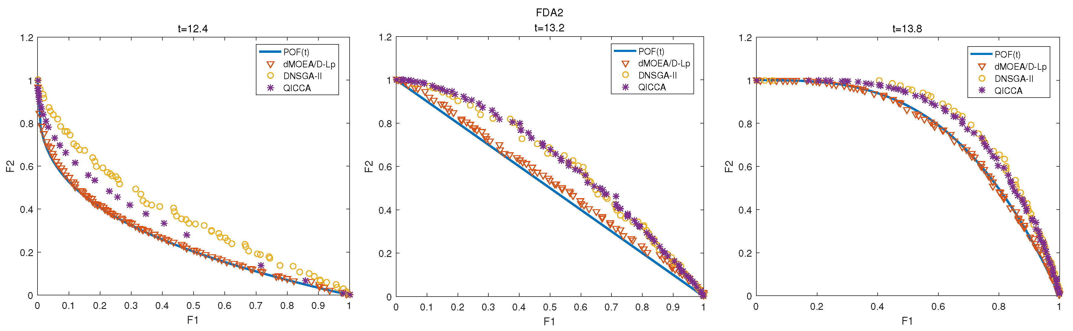
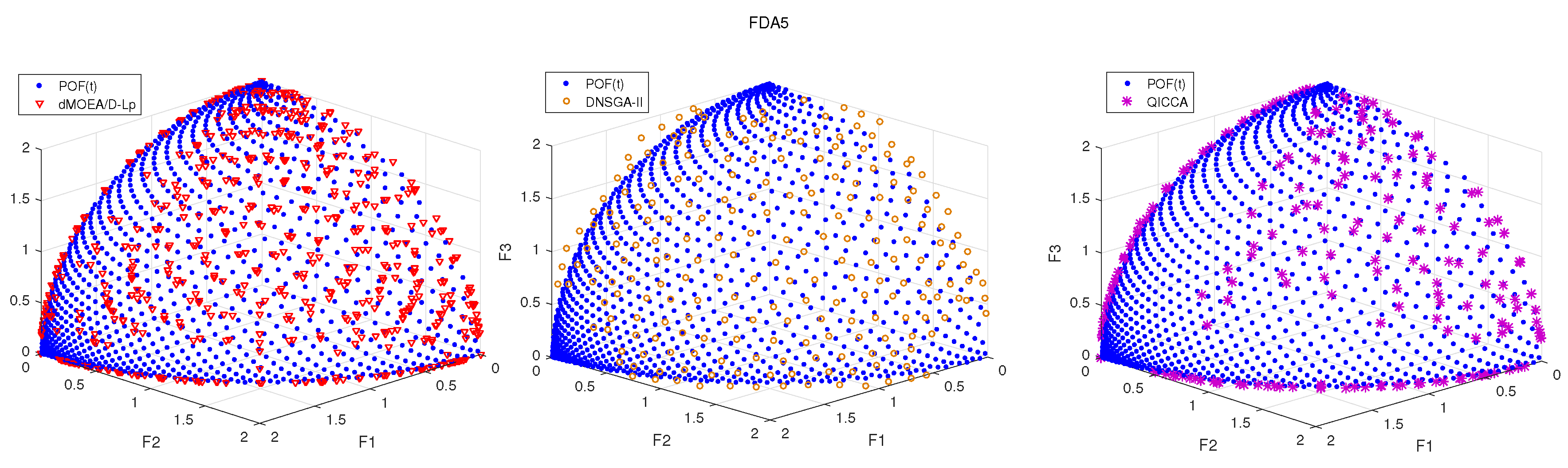
4.1. Test Problems

We used FDA benchmark test instances [3,16] and their improved versions [30,32] as our test problems. Detailed definitions of these test problems are shown in

Table 1. Test problems used in our experiments.

Problems	Objective Functions	Variable Bounds	n
FDA1	$\left\{\begin{array}{c}{f}_1(x_1)=x_1,f_2(x)=g·h\hfill \\ g(x_{II})=1+{\displaystyle \sum _{x_i\in x_{II}}}{(x_i-G(t))}^2,h(f_1,g)=1-f_{1}g\sqrt{\raisebox{1ex}{$f_1$}\!\left/ \!\raisebox{-1ex}{$g$}\right.}\hfill \\ G(t)=sin(0.5\pi t),t=⌊\tau /{\tau }_T⌋/n_T\hfill \end{array}\right.$	$\begin{array}{c}{x}_I=(x_1)\in [0,1]\hfill \\ x_{II}=(x_2,\dots ,x_n)\in [-1,1]\hfill \end{array}$	20
FDA2	$\left\{\begin{array}{c}{f}_1(x_1)=x_1,f_2(x)=g·h\hfill \\ g(x_{II})=1+{\displaystyle \sum _{x_i\in x_{II}}}{x}_i^2,h(x_{III}{f}_1,g)=1-(\raisebox{1ex}{$f_1$}\!\left/ \!\raisebox{-1ex}{$g$}\right.{)}^{2^{\left(H(t)+{\displaystyle \sum _{x_i\in x_{III}}}{(x_i-H(t)/4}^2\right)}}\hfill \\ H(t)=2sin(0.5\pi t-1),t=⌊\tau /{\tau }_T⌋/n_T\hfill \end{array}\right.$	$\begin{array}{c}{x}_I=(x_1)\in [0,1]\hfill \\ x_{II}=(x_2,\dots ,x_6)\in [-1,1]\hfill \\ x_{III}=(x_7,\dots ,x_n)\in [-1,1]\hfill \end{array}$	20
FDA3	$\left\{\begin{array}{c}{f}_1(x_1)={x_1}^{F(t)},f_2(x)=g·h\hfill \\ g(x_{II})=1+G(t)+{\displaystyle \sum _{x_i\in x_{II}}}{(x_i-G(t))}^2,h(f_1,g)=1-\sqrt{\raisebox{1ex}{$f_1$}\!\left/ \!\raisebox{-1ex}{$g$}\right.}\hfill \\ G(t)=\left|sin(0.5\pi t)\right|,F(t)={10}^{2sin(0.5\pi t)},t=⌊\tau /{\tau }_T⌋/n_T\hfill \end{array}\right.$	$\begin{array}{c}{x}_I=(x_1)\in [0,1]\hfill \\ x_{II}=(x_2,\dots ,x_n)\in [-1,1]\hfill \end{array}$	30
FDA4	$\{\begin{array}{c}{f}_1(x)=(1+g(x_{II}))\underset{i=1}{\overset{m-1}{\Pi }}cos(0.5\pi t{x}_i)\hfill \\ \begin{array}{c}{f}_k(x)=(1+g(x_{II}))\left(\underset{i=1}{\overset{m-k}{\Pi }}cos(0.5\pi t{x}_i)\right)sin(0.5\pi t{x}_{m-k+1}),k=2:m-1\hfill \\ f_m(x)=(1+g(x_{II}))sin(0.5\pi x_1)\hfill \end{array}\hfill \\ g(x_{II})={\displaystyle \sum _{x_i\in x_{II}}}{(x_i-G(t))}^2,G(t)=\left|sin(0.5\pi t)\right|,t=⌊\tau /{\tau }_T⌋/n_T\hfill \end{array}$	$\begin{array}{c}{x}_{II}=(x_m,\dots ,x_n)\hfill \\ x_i\in [0,1],i=1:n\hfill \end{array}$	12
FDA5	$\{\begin{array}{c}{f}_1(x)=(1+g(x_{II}))\underset{i=1}{\overset{m-1}{\Pi }}cos(0.5\pi t{y}_i)\hfill \\ \begin{array}{c}{f}_k(x)=(1+g(x_{II}))\left(\underset{i=1}{\overset{m-k}{\Pi }}cos(0.5\pi t{y}_i)\right)sin(0.5\pi t{y}_{m-k+1}),k=2:m-1\hfill \\ f_m(x)=(1+g(x_{II}))sin(0.5\pi y_1)\hfill \end{array}\hfill \\ \begin{array}{c}g(x_{II})=G(t)+{\displaystyle \sum _{x_i\in x_{II}}}{(x_i-G(t))}^2,G(t)=\left|sin(0.5\pi t)\right|\hfill \\ y_i={x_i}^{F(t)},i=1,\dots ,(m-1),F(t)=1+100{sin}^4(0.5\pi t)\hfill \\ t=⌊\tau /{\tau }_T⌋/n_T\hfill \end{array}\hfill \end{array}$	$\begin{array}{c}{x}_{II}=(x_m,\dots ,x_n)\hfill \\ x_i\in [0,1],i=1:n\hfill \end{array}$	12

. When the intensity of environmental change ($n_T$) is relatively small, the environmental change is less intense, and the number of POF$(t)$ is less in each cycle. When the $n_T$ value is large, the environmental change is more intense, and there will be many different POF$(t)$ in each cycle.

4.2. Performance Metric

The dynamic inverse generation distance rGD(t) [33] and dynamic generation distance GD(t) [34,35] are used as the performance evaluation metrics of the DEMOAs, and are defined as follows, respectively:

$$\begin{array}{c}\mathrm{rGD}(t)=\frac{{\sum }_{i=1}^{\left|PO{F}^{\ast }(t)\right|}{d}_i}{\left|PO{F}^{\ast }(t)\right|},d_i=\underset{k=1}{\overset{\left|Q(t)\right|}{min}}\sqrt{{{\sum }_{j=1}^m(f_j^{\ast (i)}-f_j^{(k)})}^2},\hfill \end{array}$$

(8)

$$\begin{array}{c}\mathrm{GD}(t)=\frac{\sqrt{{\sum }_{i=1}^{\left|Q(t)\right|}{(d_i^{\prime })}^2}}{\left|Q(t)\right|},d_i^{\prime }=\underset{k=1}{\overset{\left|PO{F}^{\ast }(t)\right|}{min}}\sqrt{{{\sum }_{j=1}^m(f_j^{(i)}-f_j^{\ast (k)})}^2},\hfill \end{array}$$

(9)

where $PO{F}^{\ast }(t)$ is a set of uniformly distributed points in the objective space along the $POF$ at time t, $Q(t)$ is an approximation set to the $POF$ obtained by the algorithm at the same time t, $f_j^{\ast (i)}$ is the j-th objective function value of the i-th sampling point in $PO{F}^{\ast }(t)$, and $f_j^{(i)}$ is the j-th objective function value of the i-th point in $Q(t)$.

Moreover, $d_i$ is the minimum Euclidean distance between point i of $PO{F}^{\ast }(t)$ and the points in $Q(t)$. In a sense, if the $|PO{F}^{\ast }(t)|$ is sufficiently large to represent the $PO{F}^{\ast }(t)$ very well, rGD(t) can measure both the diversity and convergence of $Q(t)$. To have a low value of rGD(t), $Q(t)$ must be very close to the $PO{F}^{\ast }(t)$, and cannot miss any part of the $PO{F}^{\ast }(t)$. Therefore, the value of rGD(t) is smaller, which means that the convergence and diversity of the obtained Pareto front is better.

$d_i^{\prime }$ is the minimum Euclidean distance between point i of $Q(t)$ and the points in $|PO{F}^{\ast }(t)|$. GD(t) measures the distance of $Q(t)$ to $PO{F}^{\ast }(t)$. The value of GD(t) is smaller, which means that the convergence and diversity of the obtained Pareto front is better. The perfect situation is that GD(t) = 0, which means that all solutions in $Q(t)$ are Pareto optimal solutions.

4.3. Setting of Experimental Parameters

Individuals used real vector encoding in all test problems. Differential evolution (DE) crossover and polynomial mutation operators [30] are adopted in the five compared algorithms (i.e., dMOEAD-$L_p$, dMOEA/D-TCH, dMOEA/D-WS, dMOEA/D-PBI and DNSGA-II) [16], where crossover rate $CR=0.9$, scaling factor $F=0.5$. The whole clone (clone ratio of 5) and non-uniform mutation is adopted in QICCA [7]; diversified introduction ratio ($\zeta$) was set to 0.2 in DNSGA-II [7]; memory pool size was set to 100. All of number of neighbors in four compared algorithms (dMOEAD-$L_p$, dMOEA/D-TCH, dMOEA/D-WS, and dMOEA/D-PBI) was set to 20; $Bsize$ was set to 5 for 2-objective problems, and to 15 for 3-objective problems; the penalty parameter ($\theta$) was set to 5 in dMOEA/D-PBI. For parameters used in the environmental monitoring operator, we took $k=2$, $\tilde{\delta }=0.002$ for problems with two objectives, and $k=3$, $\tilde{\delta }=0.006$ for 3-objective problems.

Table 2. Public parameter settings in the experiments.

Parameter	Value
Population size (N)	Two objectives: N = 100; Three objectives: N = 300
Crossover probability	0.9
Mutation probability	$1/N$
Frequency of change (${\tau }_T$)	5, 10, 15, 20, 25, 35
Severity of change ($n_T$)	5, 10

displays the common parameter settings for the compared algorithms, where n is the dimension of the decision variable. To study the effects of various dynamic changes in uncertain environments, different combinations of $({\tau }_T,n_T)$ were set according to different DMOPs. Thirty independent runs were done for each combination of the various problems. In each experiment, various algorithms uniformly tracked 100 times of environmental change. The number of generations was the combination of the environmental change time of each algorithm and the frequency of environmental change.

To choose a proper p for each test instance, we executed dMOEA/D-$L_p$ on FDA1–FDA5 with different p values: $p=0$, $p=1/3$, $p=1/2$, $p=1$, $p=2$. Experimental results are shown in

Table 3. Verification of p value in the $L_p$ decomposition method for the FDA series problem. The best performance is highlighted with bold font. rGD(t): dynamic inverse generation distance.

Problem	(${\mathit{\tau }}_{\mathit{T}}$,${\mathit{n}}_{\mathit{T}}$)	Statistic	rGD(t)
			$\mathit{p}=\infty$	$\mathit{p}=1/2$	$\mathit{p}=1/3$	$\mathit{p}=1$	$\mathit{p}=2$
FDA1(2)	(25,5)	Min Mean Std	(6.03 × 10${}^{-\mathbf{1}}$) (9.81 × 10${}^{-1}$) (2.55 × 10${}^{-1}$)	(8.30 × 10${}^{-1}$) (1.07 × 10${}^0$) (8.98 × 10${}^{-2}$)	(8.30 × 10${}^{-1}$) (1.07 × 10${}^0$) (8.98 × 10${}^{-2}$)	(1.98 × 10${}^0$) (2.02 × 10${}^0$) (8.11 × 10${}^{-2}$)	(6.75 × 10${}^{-1}$) (1.06 × 10${}^{-\mathbf{1}}$) (2.41 × 10${}^{-\mathbf{2}}$)
FDA2(2)	(15,5)	Min Mean Std	(1.11 × 10${}^{-1}$) (1.83 × 10${}^{-1}$) (7.47 × 10${}^{-2}$)	(9.33 × 10${}^{-1}$) (1.56 × 10${}^0$) (5.30 × 10${}^{-1}$)	(9.33 × 10${}^{-1}$) (1.56 × 10${}^0$) (5.30 × 10${}^{-1}$)	(2.10 × 10${}^0$) (2.91 × 10${}^0$) (4.20 × 10${}^{-1}$)	(6.33 × 10${}^{-\mathbf{2}}$) (7.34 × 10${}^{-\mathbf{2}}$) (5.04 × 10${}^{-\mathbf{3}}$)
FDA3(2)	(35,5)	Min Mean Std	(4.13 × 10${}^{-\mathbf{1}}$) (4.60 × 10${}^{-\mathbf{1}}$) (1.84 × 10${}^{-1}$)	(6.94 × 10${}^{-1}$) (3.33 × 10${}^0$) (1.34 × 10${}^0$)	(6.94 × 10${}^{-1}$) (3.33 × 10${}^0$) (1.34 × 10${}^0$)	(5.01 × 10${}^{-1}$) (6.23 × 10${}^{-1}$) (8.71 × 10${}^{-2}$)	(4.79 × 10${}^{-1}$) (5.16 × 10${}^{-1}$) (2.73 × 10${}^{-\mathbf{2}}$)
FDA4(3)	(25,5)	Min Mean Std	(2.02 × 10${}^{-1}$) (4.64 × 10${}^{-1}$) (2.64 × 10${}^{-2}$)	(8.31 × 10${}^0$) (8.36 × 10${}^0$) (2.71 × 10${}^{-2}$)	(8.31 × 10${}^0$) (8.36 × 10${}^0$) (2.71 × 10${}^{-2}$)	(8.91 × 10${}^{-1}$) (1.03 × 10${}^0$) (6.38 × 10${}^{-2}$)	(1.30 × 10${}^{-\mathbf{1}}$) (1.35 × 10${}^{-\mathbf{1}}$) (2.51 × 10${}^{-\mathbf{2}}$)
FDA5(3)	(25,5)	Min Mean Std	(8.43 × 10${}^{-2}$) (1.02 × 10${}^{-1}$) (8.43 × 10${}^{-4}$)	(8.32 × 10${}^0$) (1.26 × 10${}^{+1}$) (2.37 × 10${}^0$)	(8.32 × 10${}^0$) (1.26 × 10${}^{+1}$) (2.37 × 10${}^0$)	(1.01 × 10${}^{-1}$) (1.69 × 10${}^{-1}$) (1.86 × 10${}^{-2}$)	(5.01 × 10${}^{-\mathbf{2}}$) (5.69 × 10${}^{-\mathbf{2}}$) (3.05 × 10${}^{-\mathbf{4}}$)

. The best performance is highlighted with bold font. It can be seen from the table that $p=2$ generally performEd the best for dMOEA/D-$L_p$ in dealing with the FDA series problems. This may be because the POFs curvature of FDA1–FDA5 are quadratic, and $p=2$ in the $L_p$ function was the most suitable according to the geometric shape of the $L_p$ function in Figure 1.

4.4. Experimental Results and Analysis

In this subsection, we carry out the two parts of the experimental results and analyses. In the experiments, the statistics of the performance metrics were based on 30 independent runs.

(1)

Compare dMOEA/D-$L_p$ with dMOEA/D-WS, dMOEA/D-TCH, and dMOEA/D-PBI

To test the effectiveness of the $L_p$ decomposition method, dMOEA/D-$L_p$ was compared with dMOEA/D-WS, dMOEA/D-TCH, and dMOEA/D-PBI on the FDA series problems. Except for the decomposition method, all the other operators were the same for all four compared algorithms. The final rGD(t)-metric statistical results are shown in

Table 4. The best, mean, and standard deviation of rGD(t) metric values obtained by dMOEA/D-$L_p$ and the other versions of dMOEA/D on test problems based on 30 independent runs. The best performance of each metric value is marked in bold. dMOEA/D-PBI: dMOEA/D with the PBI decomposition approach; dMOEA/D-TCH: dMOEA/D with the Tchebycheff decomposition approach; dMOEA/D-WS: dMOEA/D with the weighted sum decomposition approach.

Problem	(${\mathit{\tau }}_{\mathit{T}}$,${\mathit{n}}_{\mathit{T}}$)	Statistic	rGD(t) Metrics
			dMOEA/D-${\mathit{L}}_{\mathit{p}}$	dMOEA/D-TCH	dMOEA/D-WS	dMOEA/D-PBI
FDA1(2)	(10, 10)	Min Mean Std	(6.69 × 10${}^{-1}$) (1.05 × 10${}^0$) (2.39 × 10${}^{-2}$)	(5.76 × 10${}^{-1}$) (1.12 × 10${}^0$) (3.20 × 10${}^{-1}$)	(1.94 × 10${}^0$) (2.05 × 10${}^0$) (1.27 × 10${}^{-1}$)	(8.01 × 10${}^{-1}$) (1.16 × 10${}^0$) (5.13 × 10${}^{-1}$)
	(25,10)	Min Mean Std	(6.75 × 10${}^{-1}$) (7.27 × 10${}^{-1}$) (2.03 × 10${}^{-2}$)	(7.33 × 10${}^{-1}$) (1.96 × 10${}^0$) (2.32 × 10${}^{-1}$)	(1.99 × 10${}^0$) (2.01 × 10${}^0$) (3.49 × 10${}^{-2}$)	(8.01 × 10${}^{-1}$) (8.74 × 10${}^{-1}$) (2.11 × 10${}^{-1}$)
	(25,5)	Min Mean Std	(6.75 × 10${}^{-1}$) (1.06 × 10${}^{-1}$) (2.41 × 10${}^{-2}$)	(6.03 × 10${}^{-1}$) (9.81 × 10${}^{-1}$) (2.55 × 10${}^{-1}$)	(1.98 × 10${}^0$) (2.02 × 10${}^0$) (8.11 × 10${}^{-2}$)	(8.85 × 10${}^{-1}$) (9.13 × 10${}^{-1}$) (2.32 × 10${}^{-1}$)
FDA2(2)	(5,10)	Min Mean Std	(2.25 × 10${}^{-\mathbf{1}}$) (3.32 × 10${}^{-\mathbf{1}}$) (5.78 × 10${}^{-\mathbf{2}}$)	(1.79 × 10${}^0$) (2.75 × 10${}^0$) (6.91 × 10${}^0$)	(1.05 × 10${}^0$) (2.44 × 10${}^0$) (6.01 × 10${}^{-1}$)	(2.33 × 10${}^{-1}$) (1.13 × 10${}^0$) (5.25 × 10${}^{-1}$)
	(15,10)	Min Mean Std	(1.21 × 10${}^{-\mathbf{1}}$) (1.30 × 10${}^{-\mathbf{1}}$) (5.71 × 10${}^{-\mathbf{2}}$)	(3.49 × 10${}^{-1}$) (7.33 × 10${}^{-1}$) (5.69 × 10${}^{-1}$)	(1.77 × 10${}^0$) (2.74 × 10${}^0$) (6.92 × 10${}^{-1}$)	(2.33 × 10${}^{-1}$) (1.13 × 10${}^0$) (5.25 × 10${}^{-1}$)
	(15,5)	Min Mean Std	(6.33 × 10${}^{-\mathbf{2}}$) (7.34 × 10${}^{-\mathbf{2}}$) (5.04 × 10${}^{-\mathbf{3}}$)	(1.11 × 10${}^{-1}$) (1.83 × 10${}^{-1}$) (7.47 × 10${}^{-2}$)	(2.10 × 10${}^0$) (2.91 × 10${}^0$) (4.20 × 10${}^{-1}$)	(1.00 × 10${}^0$) (1.77 × 10${}^0$) (7.14 × 10${}^{-1}$)
FDA3(2)	(25,10)	Min Mean Std	(1.00 × 10${}^{-\mathbf{1}}$) (1.03 × 10${}^{-\mathbf{1}}$) (2.05 × 10${}^{-\mathbf{3}}$)	(2.64 × 10${}^{-1}$) (4.03 × 10${}^{-1}$) (2.38 × 10${}^{-3}$)	(5.74 × 10${}^{-1}$) (6.56 × 10${}^{-1}$) (2.10 × 10${}^{-2}$)	(1.51 × 10${}^{-1}$) (5.15 × 10${}^{-1}$) (2.54 × 10${}^{-1}$)
	(35,10)	Min Mean Std	(4.04 × 10${}^{-1}$) (6.05 × 10${}^{-\mathbf{1}}$) (2.73 × 10${}^{-2}$)	(6.06 × 10${}^{-1}$) (7.56 × 10${}^{-1}$) (2.05 × 10${}^{-\mathbf{2}}$)	(6.13 × 10${}^{-2}$) (7.23 × 10${}^{-2}$) (1.34 × 10${}^{-1}$)	(2.17 × 10${}^{-\mathbf{1}}$) (6.06 × 10${}^{-1}$) (2.31 × 10${}^{-1}$)
	(35,5)	Min Mean Std	(4.79 × 10${}^{-1}$) (5.16 × 10${}^{-1}$) (2.73 × 10${}^{-\mathbf{2}}$)	(4.13 × 10${}^{-1}$) (4.60 × 10${}^{-\mathbf{1}}$) (1.84 × 10${}^{-1}$)	(5.01 × 10${}^{-1}$) (6.23 × 10${}^{-1}$) (8.71 × 10${}^{-2}$)	(1.35 × 10${}^{-\mathbf{1}}$) (5.33 × 10${}^{-1}$) (2.08 × 10${}^{-1}$)
FDA4(3)	(20,10)	Min Mean Std	(1.29 × 10${}^{-\mathbf{2}}$) (2.43 × 10${}^{-\mathbf{2}}$) (5.67 × 10${}^{-\mathbf{3}}$)	(7.01 × 10${}^{-1}$) (8.00 × 10${}^{-1}$) (2.34 × 10${}^{-1}$)	(1.96 × 10${}^0$) (2.74 × 10${}^0$) (6.97 × 10${}^{-1}$)	(4.05 × 10${}^{-1}$) (4.14 × 10${}^{-1}$) (1.13 × 10${}^{-1}$)
	(25,10)	Min Mean Std	(1.26 × 10${}^{-1}$) (1.40 × 10${}^{-\mathbf{1}}$) (3.36 × 10${}^{-\mathbf{2}}$)	(7.01 × 10${}^{-1}$) (8.00 × 10${}^{-1}$) (2.34 × 10${}^{-1}$)	(1.00 × 10${}^{-\mathbf{1}}$) (2.98 × 10${}^{-1}$) (6.30 × 10${}^{-1}$)	(1.01 × 10${}^{-1}$) (3.87 × 10${}^{-1}$) (3.20 × 10${}^{-1}$)
	(25,5)	Min Mean Std	(1.30 × 10${}^{-1}$) (1.35 × 10${}^{-\mathbf{1}}$) (2.51 × 10${}^{-\mathbf{2}}$)	(2.02 × 10${}^{-1}$) (4.64 × 10${}^{-1}$) (2.64 × 10${}^{-2}$)	(8.91 × 10${}^{-1}$) (1.03 × 10${}^0$) (6.38 × 10${}^{-2}$)	(1.14 × 10${}^{-\mathbf{1}}$) (2.32 × 10${}^{-1}$) (1.03 × 10${}^{-1}$)
FDA5(3)	(20,10)	Min Mean Std	(8.22 × 10${}^{-\mathbf{2}}$) (9.05 × 10${}^{-\mathbf{2}}$) (8.43 × 10${}^{-\mathbf{4}}$)	(7.37 × 10${}^{-1}$) (9.06 × 10${}^{-1}$) (2.76 × 10${}^{-3}$)	(6.03 × 10${}^{-1}$) (8.96 × 10${}^{-1}$) (1.09 × 10${}^{-3}$)	(7.79 × 10${}^{-1}$) (9.16 × 10${}^{-1}$) (1.75 × 10${}^{-3}$)
	(25,10)	Min Mean Std	(7.83 × 10${}^{-\mathbf{2}}$) (8.86 × 10${}^{-2}$) (9.75 × 10${}^{-\mathbf{5}}$)	(8.21 × 10${}^{-2}$) (8.35 × 10${}^{-\mathbf{2}}$) (1.07 × 10${}^{-4}$)	(8.43 × 10${}^{-2}$) (8.65 × 10${}^{-2}$) (1.09 × 10${}^{-3}$)	(8.03 × 10${}^{-2}$) (8.43 × 10${}^{-2}$) (1.10 × 10${}^{-4}$)
	(25,5)	Min Mean Std	(5.01 × 10${}^{-\mathbf{2}}$) (5.69 × 10${}^{-\mathbf{2}}$) (3.05 × 10${}^{-\mathbf{4}}$)	(8.43 × 10${}^{-2}$) (1.02 × 10${}^{-1}$) (8.43 × 10${}^{-4}$)	(1.01 × 10${}^{-1}$) (1.69 × 10${}^{-1}$) (1.86 × 10${}^{-2}$)	(8.01 × 10${}^{-2}$) (1.05 × 10${}^{-1}$) (6.09 × 10${}^{-2}$)

, and the final GD(t)-metric statistical results are shown in

Table 5. The best, mean, and standard deviation of GD(t) metric values obtained by dMOEA/D-$L_p$ and the other versions of dMOEA/D on test problems based on 30 independent runs. The best performance of each metric value is marked in bold.

Problem	(${\mathit{\tau }}_{\mathit{T}}$,${\mathit{n}}_{\mathit{T}}$)	Statistic	GD(t) Metrics
			dMOEA/D-${\mathit{L}}_{\mathit{p}}$	dMOEA/D-TCH	dMOEA/D-WS	dMOEA/D-PBI
FDA1(2)	(10,10)	Min Mean Std	(5.55 × 10${}^{-4}$) (9.14 × 10${}^{-4}$) (4.79 × 10${}^{-4}$)	(5.96 × 10${}^{-4}$) (6.45 × 10${}^{-3}$) (4.45 × 10${}^{-3}$)	(7.74 × 10${}^{-4}$) (9.61 × 10${}^{-3}$) (1.77 × 10${}^{-2}$)	(9.72 × 10${}^{-4}$) (1.01 × 10${}^{-2}$) (6.49 × 10${}^{-3}$)
	(25,10)	Min Mean Std	(4.18 × 10${}^{-4}$) (1.26 × 10${}^{-3}$) (5.18 × 10${}^{-4}$)	(4.92 × 10${}^{-4}$) (1.62 × 10${}^{-3}$) (6.00 × 10${}^{-4}$)	(1.20 × 10${}^{-3}$) (1.66 × 10${}^{-3}$) (1.49 × 10${}^{-3}$)	(6.71 × 10${}^{-4}$) (3.00 × 10${}^{-3}$) (1.24 × 10${}^{-3}$)
	(25,5)	Min Mean Std	(5.97 × 10${}^{-4}$) (9.13 × 10${}^{-4}$) (4.79 × 10${}^{-4}$)	(6.26 × 10${}^{-4}$) (2.26 × 10${}^{-3}$) (1.29 × 10${}^{-3}$)	(1.12 × 10${}^{-3}$) (3.35 × 10${}^{-3}$) (6.37 × 10${}^{-3}$)	(7.64 × 10${}^{-4}$) (4.12 × 10${}^{-3}$) (1.86 × 10${}^{-3}$)
FDA2(2)	(5,10)	Min Mean Std	(7.89 × 10${}^{-\mathbf{20}}$) (5.10 × 10${}^{-\mathbf{5}}$) (4.92 × 10${}^{-3}$)	(1.20 × 10${}^{-6}$) (3.31 × 10${}^{-3}$) (2.54 × 10${}^{-3}$)	(3.16 × 10${}^{-18}$) (1.55 × 10${}^{-4}$) (1.26 × 10${}^{-\mathbf{3}}$)	(8.04 × 10${}^{-4}$) (5.79 × 10${}^{-3}$) (3.43 × 10${}^{-3}$)
	(15,10)	Min Mean Std	(6.16 × 10${}^{-\mathbf{4}}$) (2.43 × 10${}^{-3}$) (4.92 × 10${}^{-\mathbf{4}}$)	(6.70 × 10${}^{-4}$) (2.46 × 10${}^{-3}$) (1.22 × 10${}^{-3}$)	(1.02 × 10${}^{-3}$) (1.32 × 10${}^{-\mathbf{3}}$) (1.31 × 10${}^{-3}$)	(6.49 × 10${}^{-4}$) (2.57 × 10${}^{-3}$) (1.54 × 10${}^{-3}$)
	(15,5)	Min Mean Std	(7.56 × 10${}^{-4}$) (4.75 × 10${}^{-\mathbf{3}}$) (2.53 × 10${}^{-\mathbf{3}}$)	(5.99 × 10${}^{-4}$) (1.91 × 10${}^{-2}$) (1.40 × 10${}^{-2}$)	(6.02 × 10${}^{-9}$) (7.66 × 10${}^{-3}$) (1.28 × 10${}^{-2}$)	(6.60 × 10${}^{-4}$) (1.98 × 10${}^{-2}$) (1.36 × 10${}^{-2}$)
FDA3(2)	(25,10)	Min Mean Std	(1.00 × 10${}^{-\mathbf{3}}$) (3.48 × 10${}^{-\mathbf{2}}$) (3.91 × 10${}^{-2}$)	(8.07 × 10${}^{-3}$) (4.92 × 10${}^{-2}$) (7.34 × 10${}^{-2}$)	(1.00 × 10${}^{-2}$) (2.20 × 10${}^{-1}$) (1.08 × 10${}^{-1}$)	(3.37 × 10${}^{-2}$) (3.71 × 10${}^{-2}$) (4.17 × 10${}^{-2}$)
	(35,10)	Min Mean Std	(1.02 × 10${}^{-\mathbf{3}}$) (3.15 × 10${}^{-\mathbf{2}}$) (3.48 × 10${}^{-\mathbf{2}}$)	(7.56 × 10${}^{-1}$) (2.16 × 10${}^0$) (1.06 × 10${}^0$)	(5.90 × 10${}^{-3}$) (6.89 × 10${}^{-2}$) (5.35 × 10${}^{-2}$)	(3.23 × 10${}^{-3}$) (3.36 × 10${}^{-2}$) (3.87 × 10${}^{-2}$)
	(35,5)	Min Mean Std	(1.06 × 10${}^{-\mathbf{3}}$) (3.64 × 10${}^{-2}$) (3.39 × 10${}^{-\mathbf{2}}$)	(9.18 × 10${}^{-3}$) (3.90 × 10${}^{-2}$) (3.89 × 10${}^{-2}$)	(1.11 × 10${}^{-2}$) (6.67 × 10${}^{-2}$) (5.53 × 10${}^{-2}$)	(7.72 × 10${}^{-3}$) (3.63 × 10${}^{-\mathbf{2}}$) (3.48 × 10${}^{-2}$)
FDA4(3)	(20,10)	Min Mean Std	(2.13 × 10${}^{-\mathbf{2}}$) (2.16 × 10${}^{-\mathbf{2}}$) (1.68 × 10${}^{-\mathbf{4}}$)	(2.52 × 10${}^{-2}$) (2.56 × 10${}^{-2}$) (8.54 × 10${}^{-4}$)	(3.24 × 10${}^{-2}$) (4.64 × 10${}^{-2}$) (2.48 × 10${}^{-2}$)	(2.31 × 10${}^{-2}$) (2.56 × 10${}^{-2}$) (2.04 × 10${}^{-4}$)
	(25,10)	Min Mean Std	(2.51 × 10${}^{-2}$) (2.55 × 10${}^{-2}$) (1.48 × 10${}^{-\mathbf{4}}$)	(1.52 × 10${}^{-\mathbf{2}}$) (2.59 × 10${}^{-2}$) (3.08 × 10${}^{-3}$)	(3.22 × 10${}^{-2}$) (5.18 × 10${}^{-2}$) (2.53 × 10${}^{-2}$)	(2.31 × 10${}^{-2}$) (2.34 × 10${}^{-\mathbf{2}}$) (1.64 × 10${}^{-4}$)
	(25,5)	Min Mean Std	(1.12 × 10${}^{-\mathbf{2}}$) (1.47 × 10${}^{-\mathbf{2}}$) (6.04 × 10${}^{-\mathbf{5}}$)	(2.53 × 10${}^{-2}$) (2.56 × 10${}^{-2}$) (1.07 × 10${}^{-4}$)	(3.21 × 10${}^{-2}$) (5.33 × 10${}^{-2}$) (3.62 × 10${}^{-2}$)	(2.31 × 10${}^{-2}$) (2.34 × 10${}^{-2}$) (1.64 × 10${}^{-4}$)
FDA5(3)	(20,10)	Min Mean Std	(2.69 × 10${}^{-2}$) (4.26 × 10${}^{-2}$) (8.35 × 10${}^{-\mathbf{3}}$)	(2.20 × 10${}^{-\mathbf{2}}$) (3.99 × 10${}^{-2}$) (1.16 × 10${}^{-2}$)	(3.23 × 10${}^{-2}$) (7.14 × 10${}^{-2}$) (3.11 × 10${}^{-2}$)	(5.76 × 10${}^{-2}$) (3.25 × 10${}^{-\mathbf{2}}$) (7.09 × 10${}^{-2}$)
	(25,10)	Min Mean Std	(2.68 × 10${}^{-2}$) (4.23 × 10${}^{-2}$) (8.30 × 10${}^{-\mathbf{4}}$)	(1.96 × 10${}^{-\mathbf{2}}$) (3.62 × 10${}^{-2}$) (7.29 × 10${}^{-3}$)	(3.42 × 10${}^{-2}$) (6.38 × 10${}^{-2}$) (2.28 × 10${}^{-3}$)	(2.56 × 10${}^{-2}$) (3.83 × 10${}^{-\mathbf{2}}$) (1.81 × 10${}^{-2}$)
	(25,5)	Min Mean Std	(2.86 × 10${}^{-2}$) (4.21 × 10${}^{-2}$) (7.85 × 10${}^{-\mathbf{4}}$)	(2.22 × 10${}^{-\mathbf{2}}$) (4.19 × 10${}^{-2}$) (8.84 × 10${}^{-4}$)	(3.26 × 10${}^{-2}$) (9.34 × 10${}^{-2}$) (5.04 × 10${}^{-2}$)	(2.82 × 10${}^{-2}$) (3.89 × 10${}^{-\mathbf{2}}$) (8.11 × 10${}^{-3}$)

. Each table includes the best, mean, and standard deviation (std) of the performance metric values, and the best performance of the metric value is highlighted in bold. As shown in Table 4, in terms of the rGD(t)-metric, we can see that dMOEA/D-$L_p$ achieved the best performance out of these four algorithms. In terms of the GD(t)-metric, the same situations occur in Table 5. The best and the mean metric values in Table 4 and Table 5 are mainly focused on dMOEA/D-$L_p$, indicating that dMOEA/D-$L_p$ behaved the best in almost all the test instances. The minimal std values obtained by dMOEA/D-$L_p$ presented the best stability of the algorithm. We can conclude that the $L_p$ decomposition method is effective and has some advantages over TCH, WS, and PBI decomposition approaches for decomposition-based dynamic multi-objective optimization.

In the $L_p$ decomposition method, $p\in (0,\infty ]$, when $p=1$, $g^{L_p}$ becomes the weighted sum method, and when $p=\infty$, $g^{L_p}$ becomes the standard Tchebycheff function. Figure 1 draws the contour lines of the $L_p$ function with different p values showing that the search ability of $L_p$ function decreased with the increase of p. All the $g^{L_p}$ functions suffered from the geometry issue except for the Tchebycheff function. Especially, a $g^{L_p}$ function cannot identify the whole Pareto optimal front of an MOP when the curvature of the Pareto optimal front is larger than the curvature of the contour line of the chosen $g^{L_p}$ function. Since the curvature of the Tchebycheff function is ∞, it is able to identify Pareto optimal solutions for any type of geometry. Overall, for a $g^{L_p}$ scalar function, its search ability and its robustness on problem geometries is a trade-off. The higher the search ability, the lower the robustness. If we can estimate the curvature of the Pareto optimal front in advance, then we can easily select a suitable $g^{L_p}$ function based on its search ability. Based on our trial experiments on p for the FDA series problem in Section 4.3, p was set to 2 in advance for dMOEA/D-$L_p$ in all experiments, which is consistent with the observation that if the curvature of the Pareto optimal front is quadratic, the most suitable $g^{L_p}$ function should be the one using $p=2$ [36]. Alternatively, for a new problem or a problem having a complex geometry, the use of the Tchebycheff function is a good choice.

(2)

Compare dMOEA/D-$L_p$ with DNSGA-II [16] and QICCA [7]

In order to test the performance of the proposed dMOEA/D-$L_p$, we tested dMOEA/D-$L_p$ on each test instance, and compared the results obtained by dMOEA/D-$L_p$ with those obtained by the other two state-of-the-art algorithms: DNSGA-II [16] and QICCA [7]. Referring to the literature with open source codes of NSGA-II [21] and MOEA/D [23], we realized the DNSGA-II, QICCA, and dMOEAD-$L_p$ with C++ language programming. The final rGD(t)-metric statistical results are shown in

Table 6. The best, mean, and standard deviation of rGD(t) metric values obtained by dMOEA/D-$L_p$ and the other two compared algorithms on test problems based on 30 independent runs. The best performance of each metric value is marked in bold.

Problem	(${\mathit{\tau }}_{\mathit{T}}$,${\mathit{n}}_{\mathit{T}}$)	Statistic	rGD(t) Metrics
			dMOEA/D-${\mathit{L}}_{\mathit{p}}$	DNSGA-II	QICCA
FDA1(2)	(10,10)	Min Mean Std	(6.69 × 10${}^{-1}$) (1.05 × 10${}^0$) (2.39 × 10${}^{-2}$)	(1.115 × 10${}^0$) (1.21 × 10${}^0$) (3.11 × 10${}^{-1}$)	(1.05 × 10${}^0$) (1.08 × 10${}^0$) (2.45 × 10${}^{-1}$)
	(25,10)	Min Mean Std	(6.75 × 10${}^{-1}$) (7.27 × 10${}^{-1}$) (2.03 × 10${}^{-2}$)	(1.07 × 10${}^0$) (1.08 × 10${}^0$) (5.48 × 10${}^{-2}$)	(1.05 × 10${}^0$) (1.06 × 10${}^0$) (4.43 × 10${}^{-2}$)
	(25,5)	Min Mean Std	(6.75 × 10${}^{-1}$) (1.06 × 10${}^0$) (2.41 × 10${}^{-2}$)	(1.06 × 10${}^0$) (1.09 × 10${}^0$) (1.36 × 10${}^{-1}$)	(1.06 × 10${}^0$) (1.07 × 10${}^0$) (7.44 × 10${}^{-2}$)
FDA2(2)	(5,10)	Min Mean Std	(2.25 × 10${}^{-\mathbf{1}}$) (3.32 × 10${}^{-\mathbf{1}}$) (5.78 × 10${}^{-\mathbf{2}}$)	(1.50 × 10${}^0$) (3.65 × 10${}^0$) (7.53 × 10${}^{-1}$)	(1.07 × 10${}^0$) (3.32 × 10${}^0$) (7.11 × 10${}^{-1}$)
	(15,10)	Min Mean Std	(1.21 × 10${}^{-\mathbf{1}}$) (1.30 × 10${}^{-\mathbf{1}}$) (5.71 × 10${}^{-\mathbf{2}}$)	(1.34 × 10${}^0$) (4.30 × 10${}^0$) (5.95 × 10${}^{-1}$)	(1.47 × 10${}^0$) (3.95 × 10${}^0$) (6.36 × 10${}^{-1}$)
	(15,5)	Min Mean Std	(6.33 × 10${}^{-\mathbf{2}}$) (7.34 × 10${}^{-\mathbf{2}}$) (5.04 × 10${}^{-\mathbf{3}}$)	(1.88 × 10${}^0$) (3.75 × 10${}^0$) (6.33 × 10${}^{-1}$)	(1.40 × 10${}^0$) (3.63 × 10${}^0$) (6.95 × 10${}^{-1}$)
FDA3(2)	(25,10)	Min Mean Std	(1.00 × 10${}^{-\mathbf{1}}$) (1.03 × 10${}^{-\mathbf{1}}$) (2.05 × 10${}^{-\mathbf{3}}$)	(1.17 × 10${}^{-1}$) (6.36 × 10${}^{-1}$) (2.61 × 10${}^{-2}$)	(1.40 × 10${}^{-1}$) (6.40 × 10${}^{-1}$) (2.63 × 10${}^{-2}$)
	(35,10)	Min Mean Std	(4.04 × 10${}^{-\mathbf{1}}$) (6.05 × 10${}^{-\mathbf{1}}$) (2.73 × 10${}^{-2}$)	(6.30 × 10${}^{-1}$) (6.35 × 10${}^{-1}$) (2.67 × 10${}^{-\mathbf{2}}$)	(6.35 × 10${}^{-1}$) (6.38 × 10${}^{-1}$) (2.68 × 10${}^{-2}$)
	(35,5)	Min Mean Std	(4.79 × 10${}^{-\mathbf{1}}$) (5.16 × 10${}^{-\mathbf{1}}$) (2.73 × 10${}^{-2}$)	(6.06 × 10${}^{-1}$) (6.10 × 10${}^{-1}$) (2.70 × 10${}^{-2}$)	(6.09 × 10${}^{-1}$) (6.11 × 10${}^{-1}$) (2.52 × 10${}^{-\mathbf{2}}$)
FDA4(3)	(20,10)	Min Mean Std	(2.43 × 10${}^{-\mathbf{2}}$) (1.29 × 10${}^{-\mathbf{2}}$) (5.67 × 10${}^{-\mathbf{3}}$)	(1.39 × 10${}^{-1}$) (1.40 × 10${}^{-1}$) (5.19 × 10${}^{-1}$)	(1.41 × 10${}^0$) (1.77 × 10${}^0$) (3.13 × 10${}^{-1}$)
	(25,10)	Min Mean Std	(1.26 × 10${}^{-\mathbf{1}}$) (1.40 × 10${}^{-\mathbf{1}}$) (3.36 × 10${}^{-\mathbf{2}}$)	(1.27 × 10${}^{-1}$) (1.42 × 10${}^{-1}$) (4.38 × 10${}^{-1}$)	(1.38 × 10${}^{-1}$) (1.45 × 10${}^{-1}$) (3.83 × 10${}^{-2}$)
	(25,5)	Min Mean Std	(1.30 × 10${}^{-\mathbf{1}}$) (1.35 × 10${}^{-\mathbf{1}}$) (2.51 × 10${}^{-\mathbf{2}}$)	(1.32 × 10${}^{-1}$) (1.38 × 10${}^{-1}$) (3.08 × 10${}^{-2}$)	(2.02 × 10${}^{-1}$) (2.29 × 10${}^0$) (5.98 × 10${}^{-2}$)
FDA5(3)	(20,10)	Min Mean Std	(8.22 × 10${}^{-2}$) (9.05 × 10${}^{-\mathbf{2}}$) (8.43 × 10${}^{-\mathbf{4}}$)	(7.31 × 10${}^{-1}$) (9.73 × 10${}^{-1}$) (3.16 × 10${}^{-3}$)	(8.03 × 10${}^{-\mathbf{2}}$) (9.13 × 10${}^{-2}$) (4.86 × 10${}^{-3}$)
	(25,10)	Min Mean Std	(8.43 × 10${}^{-2}$) (9.16 × 10${}^{-2}$) (1.07 × 10${}^{-\mathbf{4}}$)	(6.36 × 10${}^{-\mathbf{2}}$) (8.65 × 10${}^{-2}$) (1.55 × 10${}^{-4}$)	(7.91 × 10${}^{-2}$) (8.43 × 10${}^{-\mathbf{2}}$) (1.10 × 10${}^{-4}$)
	(25,5)	Min Mean Std	(5.01 × 10${}^{-\mathbf{2}}$) (5.69 × 10${}^{-\mathbf{2}}$) (3.05 × 10${}^{-\mathbf{4}}$)	(8.00 × 10${}^{-2}$) (1.06 × 10${}^{-1}$) (5.43 × 10${}^{-4}$)	(9.38 × 10${}^{-2}$) (1.05 × 10${}^{-1}$) (6.09 × 10${}^{-4}$)

, and the final GD(t)-metric statistical results are shown in

Table 7. The best, mean, and standard deviation of GD(t) metric values obtained by dMOEA/D-$L_p$ and the other two compared algorithms on test problems based on 30 independent runs. The best performance of each metric value is marked in bold.

Problem	(${\mathit{\tau }}_{\mathit{T}}$,${\mathit{n}}_{\mathit{T}}$)	Statistic	GD(t) Metrics
			dMOEA/D-${\mathit{L}}_{\mathit{p}}$	DNSGA-II	QICCA
FDA1(2)	(10,10)	Min Mean Std	(5.55 × 10${}^{-4}$) (9.14 × 10${}^{-4}$) (4.79 × 10${}^{-4}$)	(6.91 × 10${}^{-3}$) (8.08 × 10${}^{-3}$) (7.00 × 10${}^{-3}$)	(5.76 × 10${}^{-3}$) (6.49 × 10${}^{-3}$) (6.08 × 10${}^{-2}$)
	(25,10)	Min Mean Std	(4.18 × 10${}^{-4}$) (1.26 × 10${}^{-3}$) (5.18 × 10${}^{-4}$)	(1.81 × 10${}^{-3}$) (2.02 × 10${}^{-3}$) (6.42 × 10${}^{-4}$)	(1.93 × 10${}^{-3}$) (2.05 × 10${}^{-3}$) (1.37 × 10${}^{-3}$)
	(25,5)	Min Mean Std	(5.97 × 10${}^{-4}$) (9.13 × 10${}^{-4}$) (4.79 × 10${}^{-4}$)	(2.56 × 10${}^{-3}$) (2.97 × 10${}^{-3}$) (3.75 × 10${}^{-3}$)	(2.76 × 10${}^{-3}$) (2.92 × 10${}^{-3}$) (2.56 × 10${}^{-3}$)
FDA2(2)	(5,10)	Min Mean Std	(7.89 × 10${}^{-20}$) (5.10 × 10${}^{-\mathbf{5}}$) (4.92 × 10${}^{-3}$)	(1.52 × 10${}^{-\mathbf{20}}$) (1.50 × 10${}^{-3}$) (2.33 × 10${}^{-\mathbf{3}}$)	(5.10 × 10${}^{-5}$) (2.51 × 10${}^{-3}$) (2.97 × 10${}^{-3}$)
	(15,10)	Min Mean Std	(6.16 × 10${}^{-4}$) (2.43 × 10${}^{-\mathbf{3}}$) (4.92 × 10${}^{-\mathbf{4}}$)	(8.80 × 10${}^{-\mathbf{5}}$) (4.37 × 10${}^{-3}$) (3.82 × 10${}^{-3}$)	(9.11 × 10${}^{-5}$) (7.08 × 10${}^{-3}$) (5.44 × 10${}^{-3}$)
	(15,5)	Min Mean Std	(7.56 × 10${}^{-4}$) (4.75 × 10${}^{-\mathbf{3}}$) (2.53 × 10${}^{-\mathbf{3}}$)	(1.02 × 10${}^{-\mathbf{7}}$) (7.55 × 10${}^{-3}$) (5.70 × 10${}^{-3}$)	(2.43 × 10${}^{-7}$) (1.80 × 10${}^{-2}$) (1.29 × 10${}^{-2}$)
FDA3(2)	(25,10)	Min Mean Std	(1.00 × 10${}^{-\mathbf{3}}$) (3.48 × 10${}^{-\mathbf{2}}$) (3.91 × 10${}^{-\mathbf{2}}$)	(8.07 × 10${}^{-3}$) (4.92 × 10${}^{-2}$) (7.34 × 10${}^{-2}$)	(1.00 × 10${}^{-2}$) (2.20 × 10${}^{-1}$) (1.08 × 10${}^{-1}$)
	(35,10)	Min Mean Std	(1.02 × 10${}^{-\mathbf{3}}$) (3.15 × 10${}^{-\mathbf{2}}$) (3.48 × 10${}^{-\mathbf{2}}$)	(3.02 × 10${}^{-2}$) (3.23 × 10${}^{-2}$) (3.50 × 10${}^{-2}$)	(3.40 × 10${}^{-2}$) (3.68 × 10${}^{-2}$) (4.32 × 10${}^{-2}$)
	(35,5)	Min Mean Std	(1.06 × 10${}^{-\mathbf{3}}$) (3.64 × 10${}^{-\mathbf{2}}$) (3.39 × 10${}^{-\mathbf{2}}$)	(3.79 × 10${}^{-2}$) (3.92 × 10${}^{-2}$) (3.42 × 10${}^{-2}$)	(4.05 × 10${}^{-2}$) (4.27 × 10${}^{-2}$) (4.55 × 10${}^{-2}$)
FDA4(3)	(20,10)	Min Mean Std	(2.13 × 10${}^{-\mathbf{2}}$) (2.16 × 10${}^{-\mathbf{2}}$) (1.68 × 10${}^{-\mathbf{4}}$)	(3.57 × 10${}^{-2}$) (3.88 × 10${}^{-2}$) (2.03 × 10${}^{-4}$)	(2.54 × 10${}^{-2}$) (2.66 × 10${}^{-2}$) (1.83 × 10${}^{-4}$)
	(25,10)	Min Mean Std	(2.51 × 10${}^{-2}$) (2.55 × 10${}^{-\mathbf{2}}$) (1.48 × 10${}^{-\mathbf{4}}$)	(2.56 × 10${}^{-2}$) (3.11 × 10${}^{-2}$) (1.75 × 10${}^{-3}$)	(2.43 × 10${}^{-\mathbf{2}}$) (3.66 × 10${}^{-2}$) (2.02 × 10${}^{-4}$)
	(25,5)	Min Mean Std	(1.12 × 10${}^{-\mathbf{2}}$) (1.47 × 10${}^{-\mathbf{2}}$) (6.04 × 10${}^{-\mathbf{5}}$)	(1.53 × 10${}^{-2}$) (1.67 × 10${}^{-2}$) (1.44 × 10${}^{-4}$)	(1.99 × 10${}^{-2}$) (2.47 × 10${}^{-2}$) (1.68 × 10${}^{-4}$)
FDA5(3)	(20,10)	Min Mean Std	(2.69 × 10${}^{-2}$) (4.26 × 10${}^{-2}$) (8.35 × 10${}^{-\mathbf{3}}$)	(2.20 × 10${}^{-\mathbf{2}}$) (3.99 × 10${}^{-\mathbf{2}}$) (1.16 × 10${}^{-2}$)	(3.23 × 10${}^{-2}$) (7.14 × 10${}^{-2}$) (3.11 × 10${}^{-2}$)
	(25,10)	Min Mean Std	(2.68 × 10${}^{-\mathbf{2}}$) (4.23 × 10${}^{-\mathbf{2}}$) (8.30 × 10${}^{-\mathbf{4}}$)	(3.44 × 10${}^{-2}$) (4.62 × 10${}^{-2}$) (8.53 × 10${}^{-3}$)	(3.67 × 10${}^{-2}$) (4.87 × 10${}^{-\mathbf{2}}$) (8.28 × 10${}^{-3}$)
	(25,5)	Min Mean Std	(2.86 × 10${}^{-2}$) (4.21 × 10${}^{-\mathbf{2}}$) (7.85 × 10${}^{-4}$)	(3.15 × 10${}^{-2}$) (4.36 × 10${}^{-2}$) (7.32 × 10${}^{-\mathbf{4}}$)	(2.22 × 10${}^{-\mathbf{2}}$) (3.38 × 10${}^{-1}$) (1.04 × 10${}^{-2}$)

. Each table includes the best, mean, and standard deviation (std) of the performance metric values, and the best performance of each metric value is marked in bold. For intuitive analysis of the performance of three algorithms, Figure 3, Figure 4, Figure 5, Figure 6 and Figure 7 describe the approximation set to the Pareto front in different times. As shown in Table 6 and Table 7, in terms of the rGD and GD-metric, dMOEA/D-$L_p$ achieved the best performance in almost all of the test instances. Compared with DNSGA-II and QICCA, dMOEA/D-$L_p$ was competitive in solving this kind of dynamic multi-objective optimization problem.

It can be seen from Table 1 that some components ($x_{II}$) of the Pareto optimal solutions in FDA1 varied sinusoidally with the function $G(t)$, so the $POS(t)$ of FDA1 changed with time. However, at any time t, $POF(t)$ is $F_2=1-\sqrt{F_1}$ and did not change with time. Figure 3 shows the solution sets obtained by three algorithms for solving FDA1 at three different times in the tenth cycle. The corresponding environmental change factors in these three moments were ${\tau }_T=10$, $n_T=10$. Figure 4 describes the solution sets obtained by three algorithms, also for FDA1, under the parameters ${\tau }_T=25$ and $n_T=10$. From the two figures, it can be seen clearly that the solution sets obtained by dMOEA/D-$L_p$ were the most uniformly convergent to $POF(t)$ in different environments. The results of the other two algorithms in mapping significantly deviated from $POF(t)$ and the distributions were uneven. Some components ($x_{III}$) of the Pareto optimal solutions in FDA2 varied sinusoidally with the function $H(t)/4$, so the $POS(t)$ of the FDA2 changed with time. Furthermore, the $POF(t)$ of FDA2 also changed with time sinusoidally because $f_2=1-{(f_1/g)}^{2^{H(t)}}$. Figure 5 shows the solution sets obtained by three algorithms for solving FDA2 at three different times in the tenth cycle. Environmental change factors were set to ${\tau }_T=15$ and $n_T=5$. It can be seen from Figure 5 that the Pareto front shape of the problem changed from convex to concave. The solutions sets obtained by dMOEA/D-$L_p$ at three different times were closest to $POF(t)$, and the convergence distribution of dMOEA/D-$L_p$ was better than the other two algorithms.

The $POS(t)$ of the FDA3 also changed with time. Its $POF(t)$ was $f_2=(1+G(t))\times (1-\sqrt{f_1/(1+G(t))})]$, and also changed with $G(t)$. Moreover, the density of the $POF(t)$ also varied with time. Figure 6 shows the distributions of the solution sets obtained by three algorithms at three different times. From left to right, the corresponding environmental change amplitude of the problem in Figure 6 varied from small to large, and the distributions of $POF(t)$ shifted from top to bottom. All three plots of Figure 6 show that the distribution and convergence of dMOEA/D-$L_p$ were the best.

Some components of FDA5’s optimal variables ($x_{II}$) changed with $G(t)$, so its $POS(t)$ changed with time. When the number of objectives m was 3, the $POF(t)$ of FDA5 was 1/8 of a sphere at any time, but the radius of the sphere varied between 1 and 2 with time t. Figure 8, Figure 9 and Figure 10 plot the solution sets obtained by three algorithms on FDA5 at three different times. The environmental change amplitude of the problem varied from large to small in the three times, and the spherical radius of the $POF(t)$ grew from 1 to 2. Figure 8, Figure 9 and Figure 10 show that dMOEA/D-$L_p$ could best track the $POF(t)$, and the convergence and distribution of the solution sets obtained by dMOEA/D-$L_p$ were obviously superior to those obtained by the other two algorithms.

The $POS(t)$ and $POF(t)$ of FDA4 were similar to FDA5, except that the spherical radius of the $POF(t)$ remained the same value (one), not varying with time t. Similar comparing results happen for FDA4, which can be seen in Figure 7. It indicates that dMOEA/D-$L_p$ performed with obvious superiority over the other two algorithms.

5. Conclusions

In order to handle dynamic multi-objective optimization problems well, a memory-enhanced dynamic multi-objective evolutionary algorithm based on $L_p$ decomposition (denoted by dMOEA/D-$L_p$) is proposed in this paper. Specifically, dMOEA/D-$L_p$ decomposes a dynamic multi-objective optimization problem into a number of dynamic scalar optimization subproblems and optimizes them simultaneously. The $L_p$ decomposition method is referred and modified to use. To skillfully monitor environmental change and quickly respond to the new environment, an improved environment detection operator is presented and a subproblem-based memory scheme is adopted which allows the evolutionary algorithm to store good solutions from old environments and reuse them as necessary.

We conducted two sets of experimental studies. In the first set of experiments, we compared dMOEA/D-$L_p$ against dMOEA/D-TCH, dMOEA/D-WS, and dMOEA/D-PBI to test the effectiveness of the $L_p$ decomposition method for dynamic multi-objective optimization. In the second set of experiments, we compared dMOEA/D-$L_p$ with two other popular algorithms (DNSGA-II and QICCA) to test the overall performance of the algorithm. Simulation results demonstrated the effectiveness of the $L_p$ decomposition method for decomposition-based dynamic multi-objective optimization. Comparison results also revealed that the proposed dMOEA/D-$L_p$ had quick tracking performance and better convergence, it was superior and preferable in solving dynamic multi-objective optimization problems.

References

- Qu, B. Evolutionary Algorithms for Solving Multi-Modal and Multi-Objective Optimization Problems. Ph.D. Thesis, Nanyang Technological University, Singapore, 2011. [Google Scholar]
- Sindhya, K.; Miettinen, K.; Deb, K. A Hybrid Framework for Evolutionary Multi-Objective Optimization. IEEE Trans. Evolut. Comput. 2013, 17, 495–511. [Google Scholar] [CrossRef]
- Farina, M.; Deb, K.; Amato, P. Dynamic multiobjective optimization problems: Test cases, approximations, and applications. IEEE Trans. Evolut. Comput. 2004, 8, 425–442. [Google Scholar] [CrossRef]
- Wu, Y.; Jin, Y.; Liu, X. A directed search strategy for evolutionary dynamic multiobjective optimization. Soft Comput. 2015, 19, 3221–3235. [Google Scholar] [CrossRef]
- Jin, Y.; Branke, J. Evolutionary optimization in uncertain environments-a survey. IEEE Trans. Evolut. Comput. 2005, 9, 303–317. [Google Scholar] [CrossRef]
- Liu, C.; Wang, Y. Dynamic Multi-objective Optimization Evolutionary Algorithm. Nat. Sci. J. Hainan Univ. 2010, 4, 456–459. [Google Scholar]
- Shang, R.; Jiao, L.; Ren, Y.; Li, L.; Wang, L. Quantum immune clonal coevolutionary algorithm for dynamic multiobjective optimization. Nat. Comput. Int. J. 2014, 13, 421–445. [Google Scholar] [CrossRef]
- Zhang, Z. Multiobjective Optimization Immune Algorithm In Dynamic Environments And Its Application To Greenhouse Control. Appl. Soft Comput. 2008, 8, 959–971. [Google Scholar] [CrossRef]
- Li, X.; Branke, J.; Kirley, M. On performance metrics and particle swarm methods for dynamic multiobjective optimization problems. In Proceedings of the IEEE Congress on Evolutionary Computation (CEC 2007), Singapore, 25–28 September 2007; pp. 576–583. [Google Scholar]
- Li, Y.; Zhan, Z.H.; Lin, S.; Zhang, J.; Luo, X. Competitive and cooperative particle swarm optimization with information sharing mechanism for global optimization problems. Inf. Sci. 2015, 293, 370–382. [Google Scholar] [CrossRef]
- Zheng, X.W.; Lu, D.J.; Wang, X.G.; Liu, H. A cooperative coevolutionary biogeography-based optimizer. Appl. Intell. 2015, 43, 95–111. [Google Scholar] [CrossRef]
- Goh, C.K.; Tan, K.C. A Competitive-Cooperative Coevolutionary Paradigm for Dynamic Multiobjective Optimization. IEEE Trans. Evolut. Comput. 2009, 13, 103–127. [Google Scholar]
- Jiang, S.; Yang, S. A Steady-state and Generational Evolutionary Algorithm for Dynamic Multiobjective Optimization. IEEE Trans. Evolut. Comput. 2017, 21, 65–82. [Google Scholar] [CrossRef]
- Wang, Y.; Li, B. Multi-strategy ensemble evolutionary algorithm for dynamic multi-objective optimization. Memet. Comput. 2010, 2, 3–24. [Google Scholar] [CrossRef]
- Chen, J.H.; Cheng, C.W. Multi-objective evolutionary optimization of dynamic service facility location problems. In Proceedings of the 2011 IEEE Southeastcon, Nashville, TN, USA, 17–20 March 2011; pp. 333–338. [Google Scholar]
- Deb, K.; Udaya, B.R.N.; Karthik, S. Dynamic Multi-objective Optimization and Decision-Making Using Modified NSGA-II: A Case Study on Hydro-thermal Power Scheduling. In Proceedings of the International Conference on Evolutionary Multi-Criterion Optimization, Matsushima, Japan, 5–8 March 2007; Springer: Berlin/Heidelberg, Germany, 2007; pp. 803–817. [Google Scholar]
- Hutzschenreuter, A.K.; Bosman, P.A.N.; Han, L.P. Evolutionary Multiobjective Optimization for Dynamic Hospital Resource Management. In Proceedings of the International Conference on Evolutionary Multi-Criterion Optimization, Nantes, France, 7–10 April 2009; Springer: Berlin/Heidelberg, Germany, 2009; pp. 320–334. [Google Scholar]
- Li, J.Q.; Sang, H.Y.; Han, Y.Y.; Wang, C.G.; Gao, K.Z. Efficient multi-objective optimization algorithm for hybrid flow shop scheduling problems with setup energy consumptions. J. Clean. Prod. 2018, 181, 584–598. [Google Scholar] [CrossRef]
- Barlow, G.J.; Smith, S.F. A Memory Enhanced Evolutionary Algorithm for Dynamic Scheduling Problems. In Workshops on Applications of Evolutionary Computation; Lecture Notes in Computer Science; Springer: Berlin/Heidelberg, Germany, 2008; Volume 4974, pp. 606–615. [Google Scholar]
- Yang, S.; Yao, X. Population-Based Incremental Learning with Associative Memory for Dynamic Environments. IEEE Trans. Evolut. Comput. 2008, 12, 542–561. [Google Scholar] [CrossRef]
- Deb, K.; Pratap, A.; Agarwal, S.; Meyarivan, T.A.M.T. A fast and elitist multiobjective genetic algorithm: NSGA-II. IEEE Trans. Evolut. Comput. 2002, 6, 182–197. [Google Scholar] [CrossRef] [Green Version]
- Koo, W.T.; Chi, K.G.; Tan, K.C. A predictive gradient strategy for multiobjective evolutionary algorithms in a fast changing environment. Memet. Comput. 2010, 2, 87–110. [Google Scholar] [CrossRef]
- Zhang, Q.; Li, H. MOEA/D: A Multiobjective Evolutionary Algorithm Based on Decomposition. IEEE Trans. Evolut. Comput. 2007, 11, 712–731. [Google Scholar] [CrossRef] [Green Version]
- Coello, C.A.C.; Lamont, G.B.; Van Veldhuizen, D.A. Evolutionary Algorithms For Solving Multi-Objective Problems; Springer: New York, NY, USA, 2007. [Google Scholar]
- Miettinen, K. Nonlinear Multiobjective Optimization; Kluwer Academic Publishers: Boston, MA, USA, 1999. [Google Scholar]
- Bai, J.; Liu, H. Multi-objective artificial bee algorithm based on decomposition by PBI method. Appl. Intell. 2016, 45, 976–991. [Google Scholar] [CrossRef]
- Branke, J. Memory enhanced evolutionary algorithms for changing optimization problems. In Proceedings of the 1999 Congress on Evolutionary Computation-CEC99, Washington, DC, USA, 6–9 July 1999; Volume 3, pp. 1875–1882. [Google Scholar]
- Das, S.; Suganthan, P.N. Differential Evolution: A Survey of the State-of-the-Art. IEEE Trans. Evolut. Comput. 2011, 15, 4–13. [Google Scholar] [CrossRef]
- Tan, Y.Y.; Jiao, Y.C.; Li, H.; Wang, X.K. A modification to MOEA/D-DE for multiobjective optimization problems with complicated Pareto sets. Inf. Sci. 2012, 213, 14–38. [Google Scholar] [CrossRef]
- Min, L. Memory Enhanced Dynamic Multi-Objective Evolutionary Algorithm Based on Decomposition. J. Softw. 2013, 24, 1571–1588. [Google Scholar]
- Liu, R.; Niu, X.; Fan, J. An orthogonal predictive model-based dynamic multi-objective optimization algorithm. Soft Comput. 2015, 19, 3083–3107. [Google Scholar] [CrossRef]
- Sola, M.C. Parallel Processing for Dynamic Multi-Objective Optimization. Ph.D. Thesis, University of Granada, Granada, Spain, 2010. [Google Scholar]
- Zitzler, E.; Thiele, L.; Laumanns, M.; Fonseca, C.M.; Da Fonseca, V.G. Performance assessment of multiobjective optimizers: An analysis and review. IEEE Trans. Evolut. Comput. 2003, 7, 117–132. [Google Scholar] [CrossRef]
- Veldhuizen, D.A.V.; Lamont, G.B. Evolutionary Computation and Convergence to a Pareto Front. In Proceedings of the Late Breaking Papers at the Genetic Programming 1998 Conference, Madison, WI, USA, 22–25 July 1998; pp. 221–228. [Google Scholar]
- Veldhuizen, D.A.V.; Lamont, G.B. Multiobjective evolutionary algorithm test suites. In Proceedings of the 1999 ACM Symposium on Applied Computing, San Antonio, TX, USA, 28 February–2 March 1999; pp. 351–357. [Google Scholar]
- Okimoto, T.; Schwind, N.; Clement, M. Lp-Norm based algorithm for multi-objective distributed constraint optimization. In Proceedings of the 2014 International Conference on Autonomous Agents and Multi-Agent Systems, Paris, France, 5–9 May 2014; Volume 18, pp. 1427–1428. [Google Scholar]