Transmission of High Frequency Vibrations in Rotating Systems. Application to Cavitation Detection in Hydraulic Turbines


Abstract
:1. Introduction
- -
- -
- -
- -
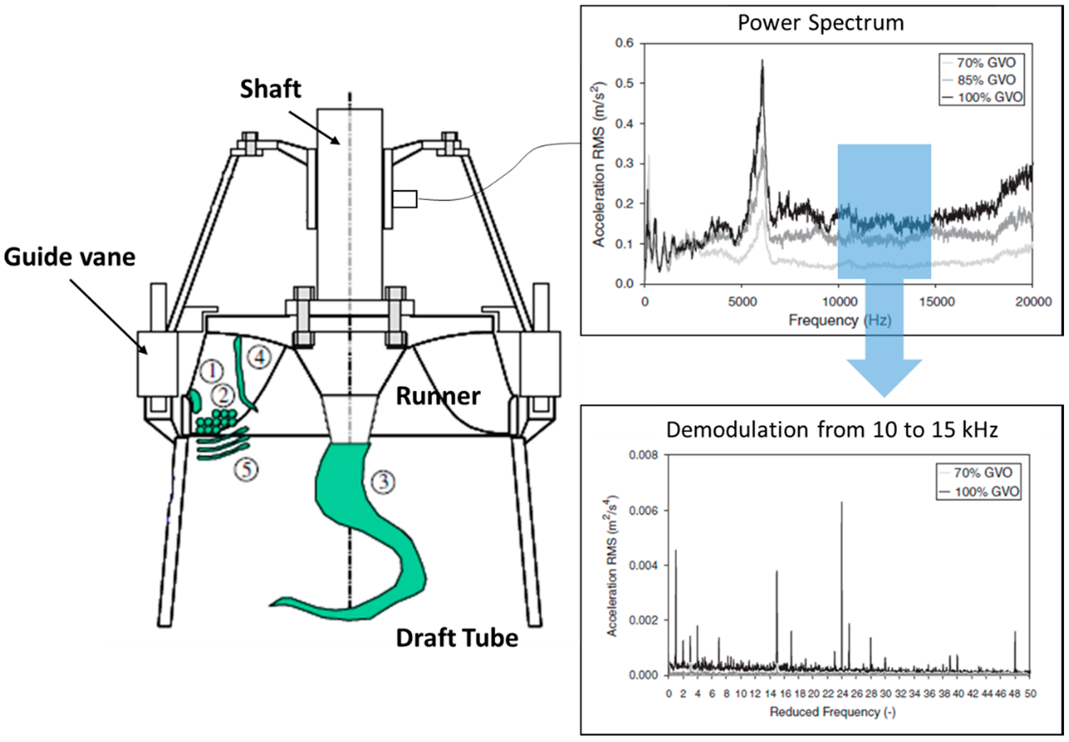
- Detection with accelerometers in the shaft [21]: Direct path from the runner, but more complicated measurement with the possibility of having also generator excitations.
- -
- The transmission path from the runner to the measuring position can only be known in air (the runner could be impacted during an overhaul [17]) but not in water and under operation.
- -
- No correlation between existing cavitation and the measured signals can be obtained: the cavitation cannot be visualized in the prototype [25].
- -
- The excitation characteristics of the cavitation are an unknown.
- -
- It is not clear which high-frequency bands have to be used for every sensor for the analysis.
2. Experimental Investigation
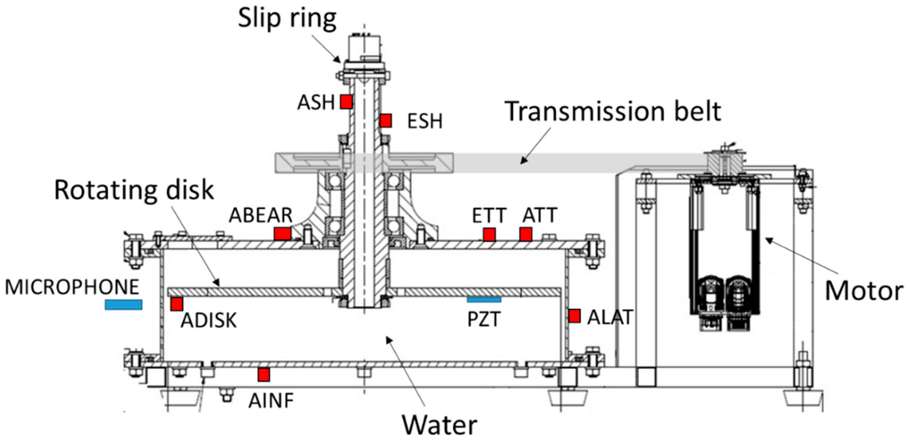
2.1. Test Rig Description
2.2. Instrumentation
2.3. Tests Conducted
2.4. Signal Analysis
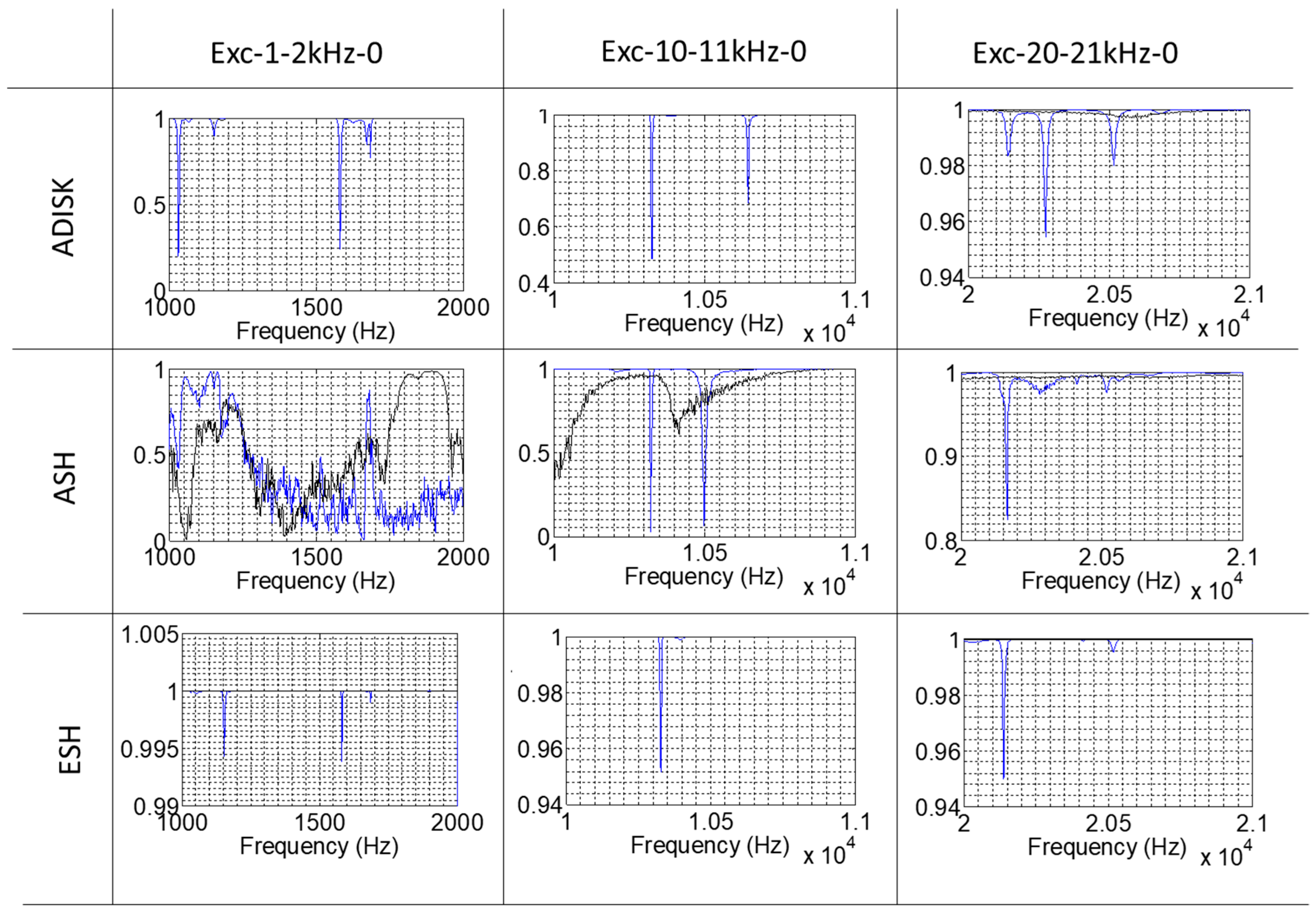
2.4.1. Coherence
2.4.2. Frequency Response Function (FRF)
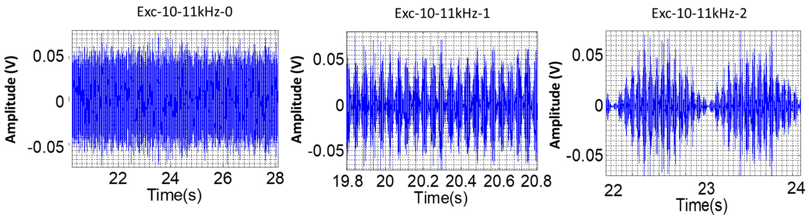
2.4.3. Amplitude Demodulation Analysis
3. Results and Discussion
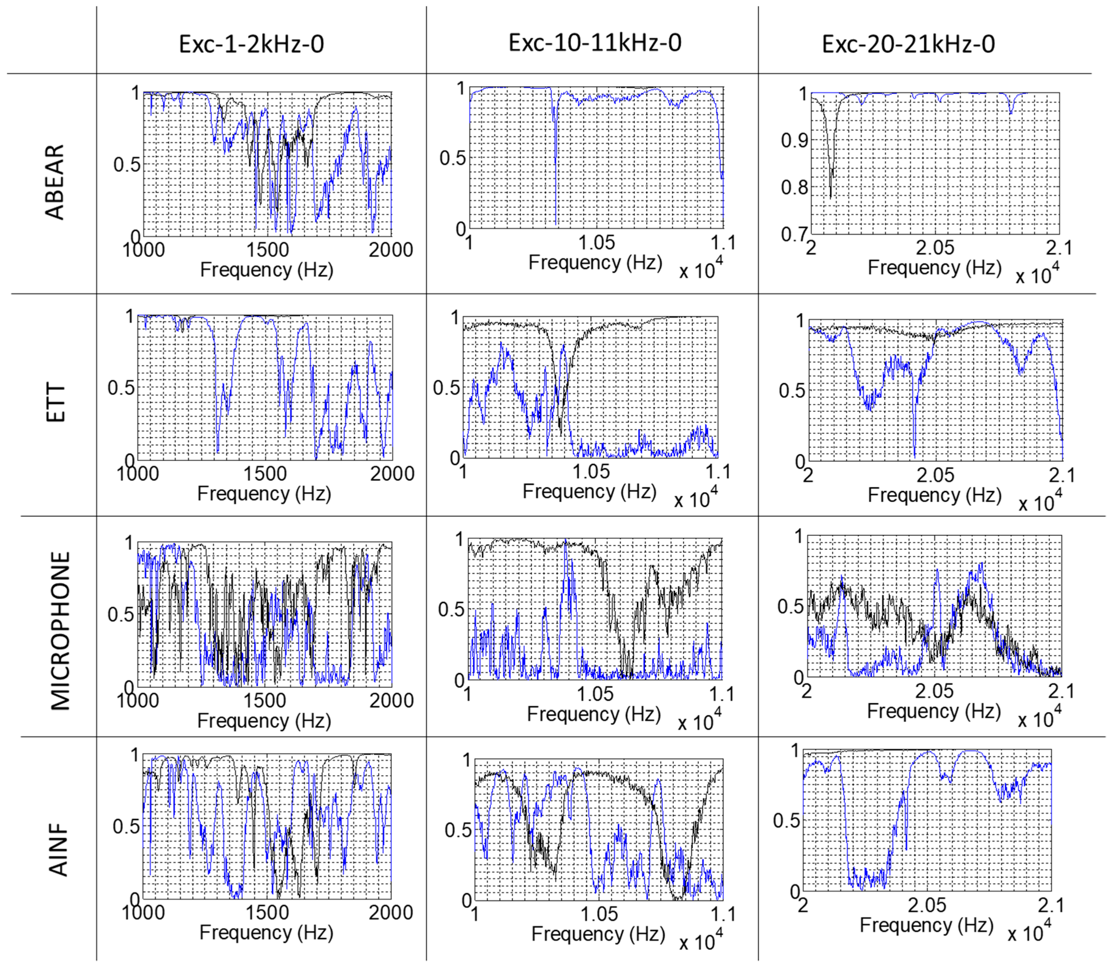
3.1. Coherence
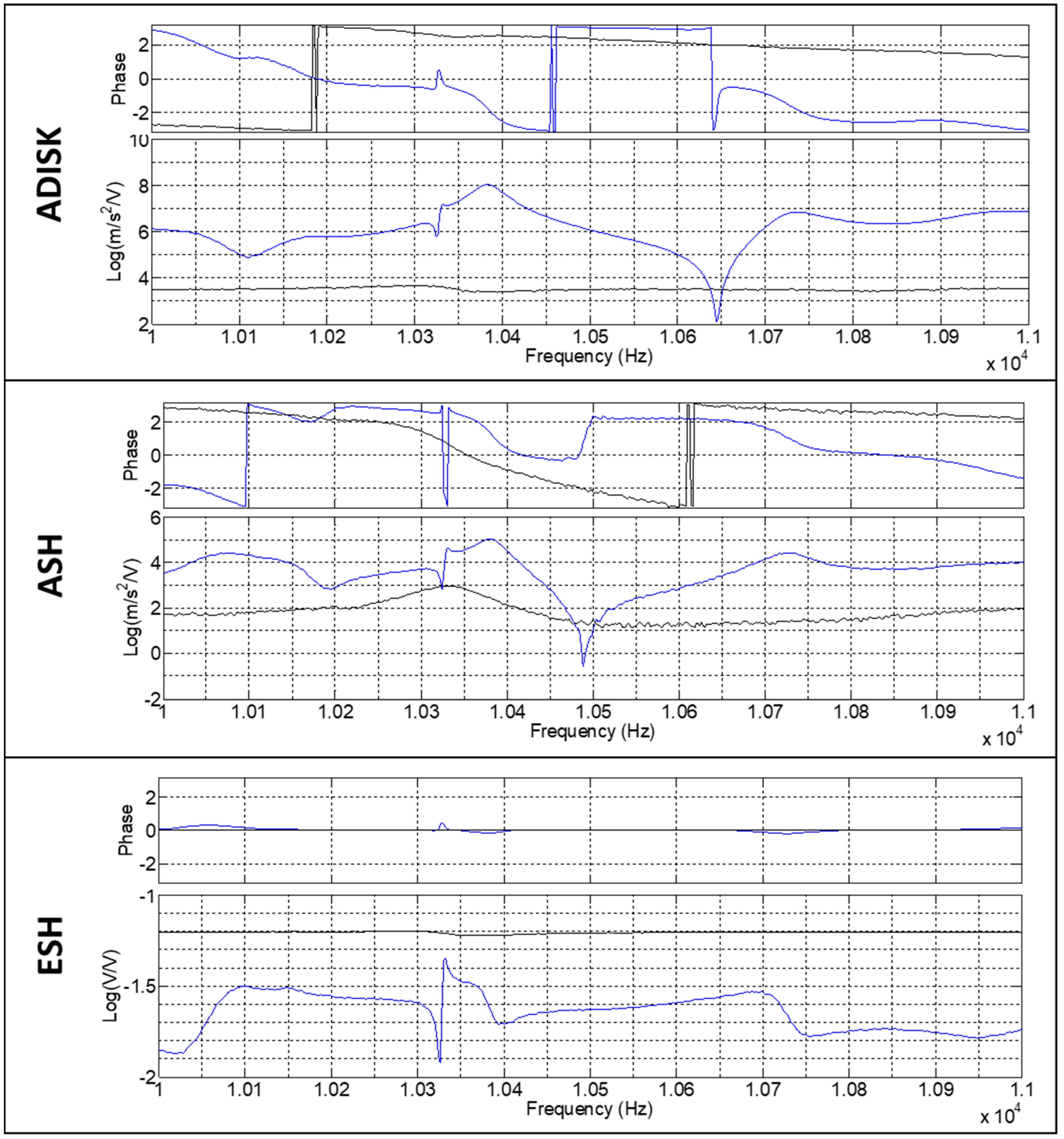
3.2. FRF
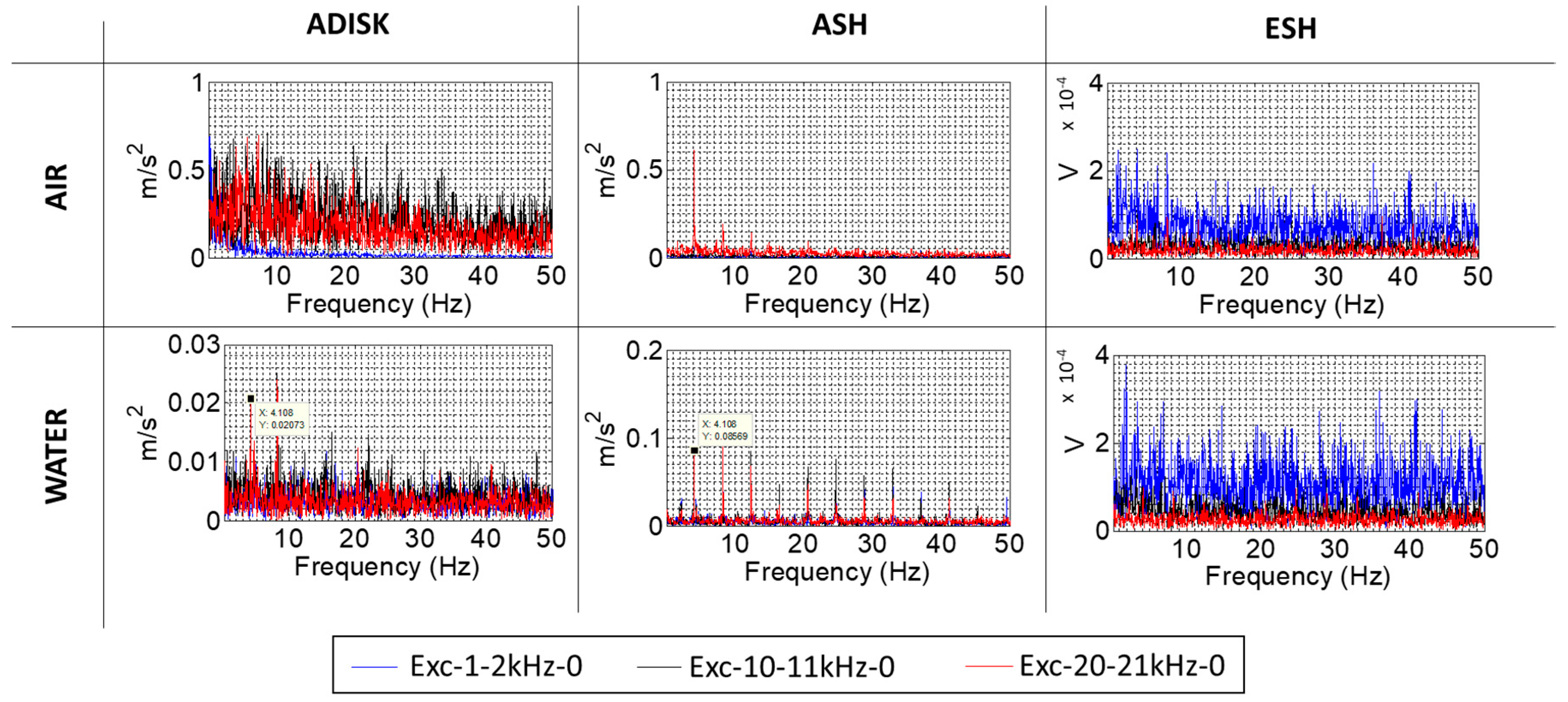
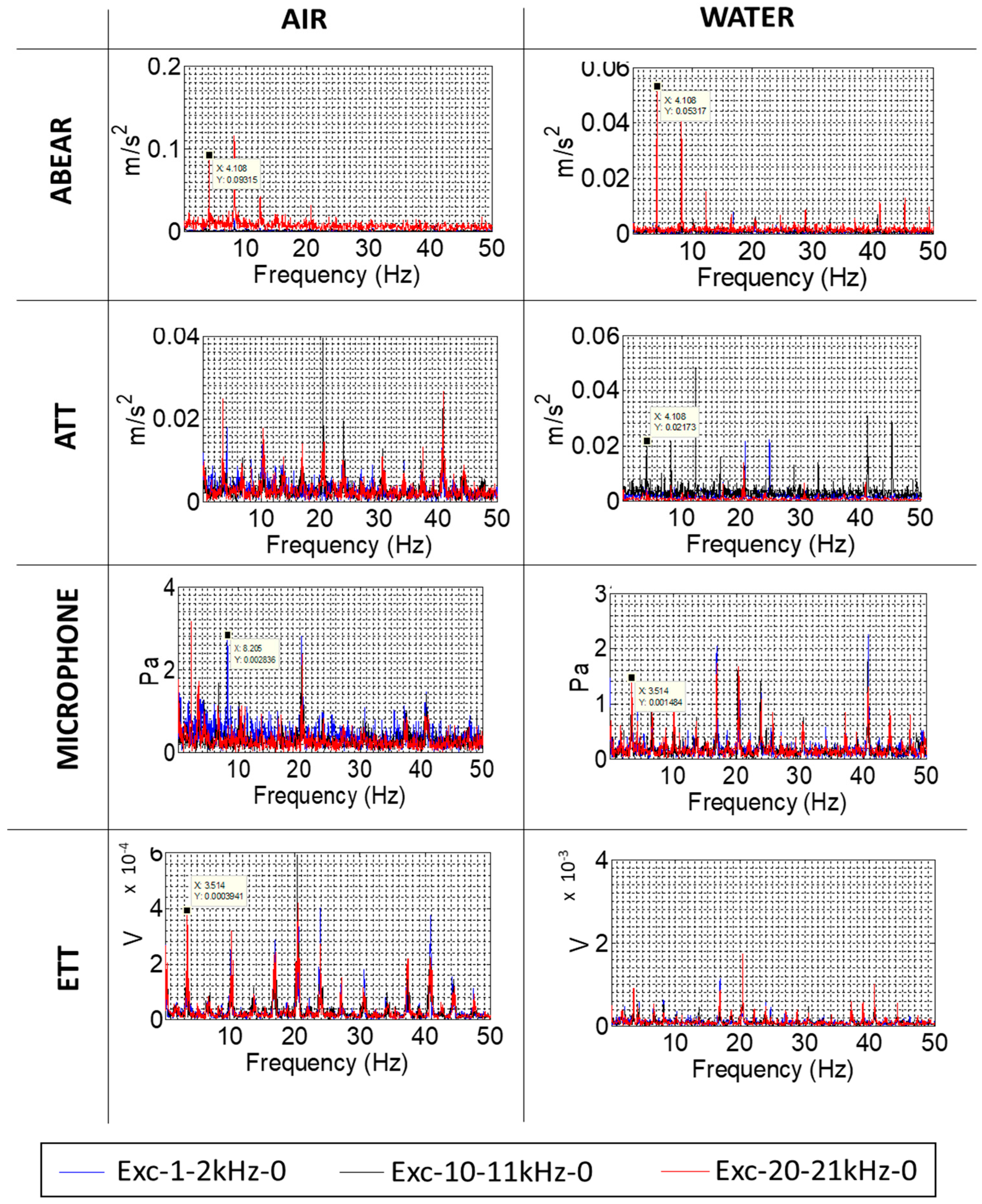
3.3. Amplitude Demodulation Analysis
3.3.1. Without Modulating Frequencies
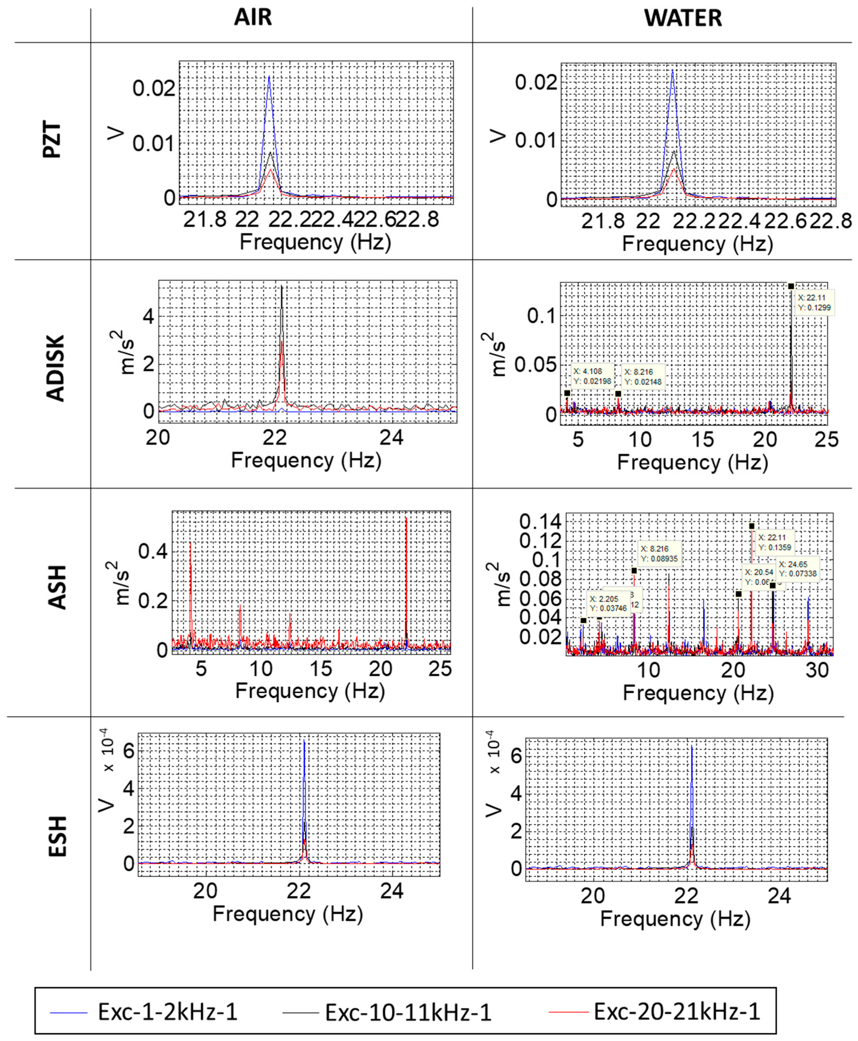
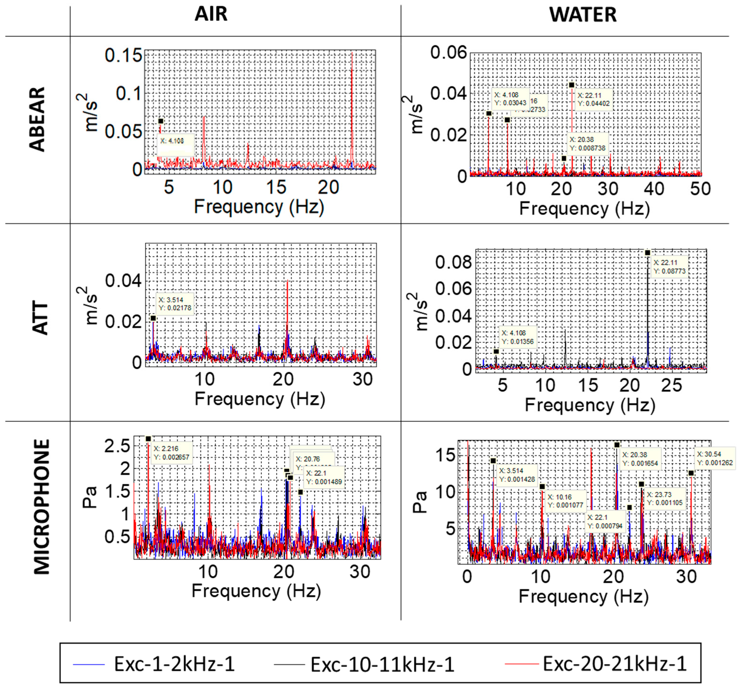
3.3.2. With One Modulating Frequency
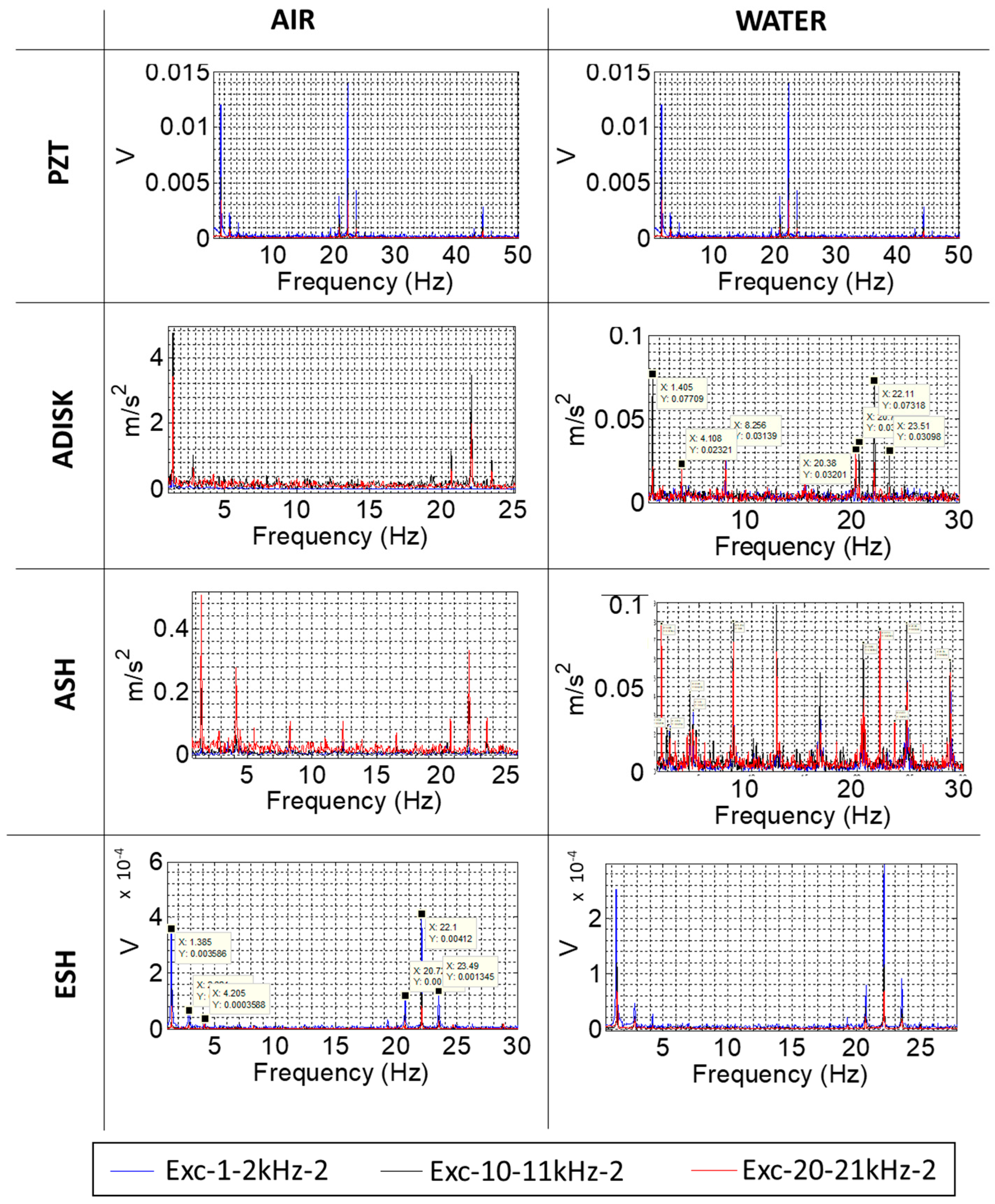
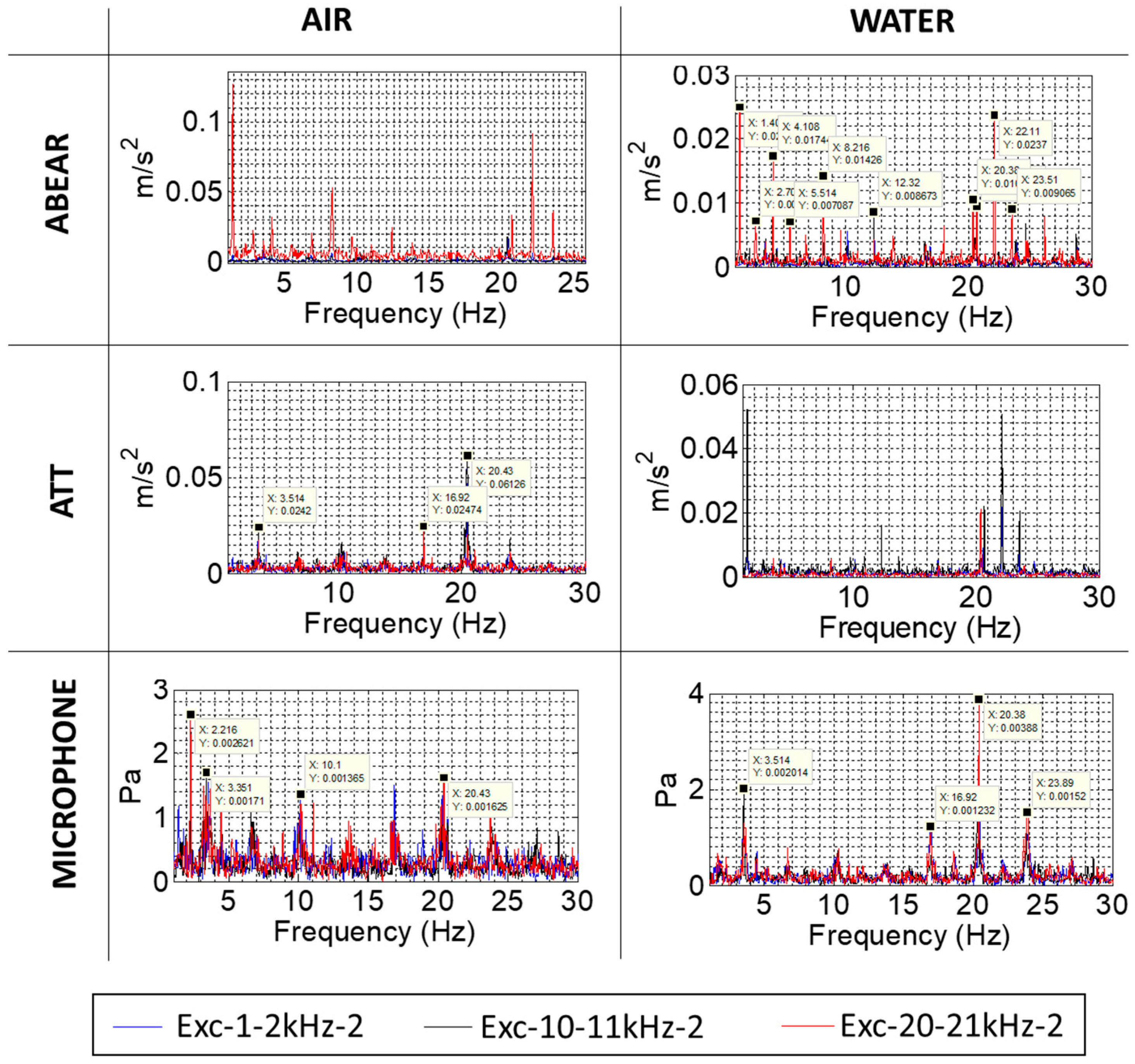
3.3.3. With Two Modulating Frequencies
4. Conclusions
Acknowledgments
Author Contributions
Conflicts of Interest
Nomenclature
| AE | Acoustic Emission |
| BEP | Best Efficiency Point |
| RMS | Root Mean Square |
| RSI | Rotor Stator Interaction |
| PS | Pseudorandom |
| PZT | Piezoelectric Patch |
| f | Frequency |
| t | Time |
| Hi | Hilbert transform |
| θ | Phase shift |
| ff | Rotating frequency |
| f1 | Modulating frequency at 22.1 Hz |
| f2 | Modulating frequency at 1.4 Hz |
| FRFH1 | Frequency Response Function |
| Sxx(f) | Power Spectra Density function of x(t) |
| Syy(f) | Power Spectra Density function of y(t) |
| Sxy(f) | Cross-spectral Density function of x(t) and y(t) |
| Variable which satisfies |
References
- Bélanger, C.; Gagnon, L. Adding wind energy to hydropower. Energy Policy 2002, 30, 1279–1284. [Google Scholar] [CrossRef]
- IEA (International Energy Agency). Key World Energy Trends. Excerpt from: World Energy Balances. 2016. Available online: www.iea.org (accessed on 10 November 2017).
- Gaudard, L.; Romerio, F. The future of hydropower in Europe: Interconnecting climate, markets and policies. Environ. Sci. Policy 2014, 37 (Suppl. C), 172–181. [Google Scholar] [CrossRef]
- Egusquiza, E.; Valero, C.; Huang, X.; Jou, E.; Guardo, A.; Rodriguez, C. Failure investigation of a large pump-turbine runner. Eng. Failure Anal. 2012, 23, 27–34. [Google Scholar] [CrossRef] [Green Version]
- Egusquiza, E.; Valero, C.; Presas, A.; Huang, X.; Guardo, A.; Seidel, U. Analysis of the dynamic response of pump-turbine impellers. Influence of the rotor. Mech. Syst. Signal Process. 2016, 68–69, 330–341. [Google Scholar] [CrossRef]
- Trivedi, C. A review on fluid structure interaction in hydraulic turbines: A focus on hydrodynamic damping. Eng. Failure Anal. 2017, 77, 1–22. [Google Scholar] [CrossRef]
- Frosina, E.; Buono, D.; Senatore, A. A Performance Prediction Method for Pumps as Turbines (PAT) Using a Computational Fluid Dynamics (CFD) Modeling Approach. Energies 2017, 10, 103. [Google Scholar] [CrossRef]
- Kumar, P.; Saini, R.P. Study of cavitation in hydro turbines—A review. Renew. Sustain. Energy Rev. 2010, 14, 374–383. [Google Scholar] [CrossRef]
- Escaler, X.; Egusquiza, E.; Farhat, M.; Avellan, F.; Coussirat, M. Detection of cavitation in hydraulic turbines. Mech. Syst. Signal Process. 2006, 20, 983–1007. [Google Scholar] [CrossRef]
- Knapp, R.; Daily, J.; Hammitt, F. Cavitation; McGraw-Hill: New York, NY, USA, 1970; Volume 2, pp. 1–20. [Google Scholar]
- Avellan, F.; Farhat, M. Shock Pressure Generated by Cavitation Vortex Collapse. ASME, San Francisco, December 1988, Proceedings of 3rd International Symposium on Cavitation Noise and Erosion in Fluid System of the ASME Winter Annual Meeting, San Fransisco, CA, USA, December 1989; EPFL Scientific Publications: Lausanne, Schweizerische; pp. 119–125.
- Favrel, A.; Müller, A.; Landry, C.; Yamamoto, K.; Avellan, F. Study of the vortex-induced pressure excitation source in a Francis turbine draft tube by particle image velocimetry. Exp. Fluids 2015, 56, 215. [Google Scholar] [CrossRef]
- Favrel, A.; Müller, A.; Landry, C.; Gomes, J.; Yamamoto, K.; Avellan, F. Dynamics of the Precessing Vortex Rope and Its Interaction with the System at Francis Turbines Part Load Operating Conditions; Journal of Physics: Conference Series, 2017; IOP Publishing: Bristol, UK, 2017; p. 012023. [Google Scholar]
- Müller, A.; Favrel, A.; Landry, C.; Avellan, F. Fluid–structure interaction mechanisms leading to dangerous power swings in Francis turbines at full load. J. Fluids Struct. 2017, 69 (Suppl. C), 56–71. [Google Scholar] [CrossRef]
- Yamamoto, K.; Müller, A.; Favrel, A.; Landry, C.; Avellan, F. Flow Characteristics and Influence Associated with Inter-Blade Cavitation Vortices at Deep Part Load Operations of a Francis Turbine; Journal of Physics: Conference Series, 2017; IOP Publishing: Bristol, UK, 2017; p. 012029. [Google Scholar]
- Avellan, F.; Dupont, P.; Ryhming, I.L. Generation Mechanism and Dynamics of Cavitation Vortices Downstream of a Fixed Leading Edge Cavity, Proceedings of the17th Symposium on Naval Hydrodynamics, The Hague, The Netherland, 28 Aguust–2 September 1988; EPFL Scientific Publications: Lausanne, Schweizerische; pp. 1–13.
- Escaler, X.; Ekanger, J.V.; Francke, H.H.; Kjeldsen, M.; Nielsen, T.K. Detection of Draft Tube Surge and Erosive Blade Cavitation in a Full-Scale Francis Turbine. J. Fluids Eng. 2014, 137, 011103. [Google Scholar] [CrossRef] [Green Version]
- Escaler, X.; Farhat, M.; Ausoni, P.; Egusquiza, E.; François, A. Cavitation Monitoring of Hydroturbines: Tests in a Francis Turbine Model; CAV2006: Wageningen, The Netherlands, 2006. [Google Scholar]
- Bajic, B. Multidimensional diagnostics of turbine cavitation. J. Fluids Eng. 2002, 124, 943–950. [Google Scholar] [CrossRef]
- Bajić, B.; Keller, A. Spectrum Normalization Method in Vibro-Acoustical Diagnostic Measurements of Hydroturbine Cavitation. J. Fluids Eng. 1996, 118, 756–761. [Google Scholar] [CrossRef]
- Escaler, X.; Egusquiza, E.; Farhat, M.; Avellan, F. Vibration Cavitation Detection Using Onboard Measurements. In Proceedings of the Fifth International Symposium on Cavitation, Osaka, Japan, 1–5 November 2003. [Google Scholar]
- Cencič, T.; Hočevar, M.; Širok, B. Study of Cavitation in Pump-Storage Hydro Power Plant Prototype. In Proceedings of the 6th IAHR Internation Meeting of the Workgroup on Cavitation and Dynamic Problems in Hydraulic Machinery and Systems, Ljubljana, Slovenia, 9–11 September 2015. [Google Scholar]
- Bourdon, P.; Simoneau, R.; Lavigne, P. A vibratory Approach to the Detection of Erosive Cavitation, Proceedings of the ASME International Symposium on Cavitation Noise and Erosion in Fluid Systems, San Francisco, CA, USA, December 1989; FED: Washington, DC, USA, 1989. [Google Scholar]
- Vizmanos, C.; Egusquiza, E.; Jou, E. Cavitation detection in a Francis turbine. Int. J. Hydropower Dams 1996, 3, 161–168. [Google Scholar]
- Escaler, X.; Farhat, M.; Egusquiza, E.; Avellan, F. Dynamics and Intensity of Erosive Partial Cavitation. J. Fluids Eng. 2007, 129, 886–893. [Google Scholar] [CrossRef]
- Presas, A.; Egusquiza, E.; Valero, C.; Valentin, D.; Seidel, U. Feasibility of Using PZT Actuators to Study the Dynamic Behavior of a Rotating Disk due to Rotor-Stator Interaction. Sensors 2014, 14, 11919–11942. [Google Scholar] [CrossRef] [PubMed] [Green Version]
- Presas, A.; Valentin, D.; Egusquiza, E.; Valero, C.; Seidel, U. Influence of the rotation on the natural frequencies of a submerged-confined disk in water. J. Sound Vib. 2015, 337, 161–180. [Google Scholar] [CrossRef]
- Presas, A.; Valentin, D.; Egusquiza, E.; Valero, C.; Seidel, U. On the detection of natural frequencies and mode shapes of submerged rotating disk-like structures from the casing. Mech. Syst. Signal Process. 2015, 60–61, 547–570. [Google Scholar] [CrossRef] [Green Version]
- Valentín, D.; Presas, A.; Egusquiza, E.; Valero, C. On the Capability of Structural–Acoustical Fluid–Structure Interaction Simulations to Predict Natural Frequencies of Rotating Disklike Structures Submerged in a Heavy Fluid. J. Vib. Acoust. 2016, 138, 034502. [Google Scholar] [CrossRef]
- Presas, A.; Valentin, D.; Egusquiza, E.; Valero, C.; Egusquiza, M.; Bossio, M. Accurate Determination of the Frequency Response Function of Submerged and Confined Structures by Using PZT-Patches. Sensors 2017, 17, 660. [Google Scholar] [CrossRef] [PubMed]
- Rodriguez, C.G.; Mateos-Prieto, B.; Egusquiza, E. Monitoring of Rotor-Stator Interaction in Pump-Turbine Using Vibrations Measured with On-Board Sensors Rotating with Shaft. Shock Vib. 2014, 2014, 8. [Google Scholar] [CrossRef]
- Egusquiza, E.; Valero, C.; Valentin, D.; Presas, A.; Rodriguez, C.G. Condition monitoring of pump-turbines. New challenges. Measurement 2015, 67, 151–163. [Google Scholar] [CrossRef] [Green Version]
- Presas, A.; Valentín, D.; Egusquiza, E.; Valero, C.; Seidel, U. Experimental analysis of the dynamic behavior of a rotating disk submerged in water. IOP Conf. Ser. Earth Environ. Sci. 2014, 22, 032043. [Google Scholar] [CrossRef]
- Presas, A.; Valentin, D.; Egusquiza, E.; Valero, C.; Seidel, U. Dynamic response of a rotating disk submerged and confined. Influence of the axial gap. J. Fluids Struct. 2016, 62, 332–349. [Google Scholar] [CrossRef]
- Presas, A.; Valentin, D.; Egusquiza, E.; Valero, C.; Seidel, U.; Weber, W. Natural Frequencies of Rotating Disk-Like Structures Submerged Viewed from the Stationary Frame; IOP Conference Series: Earth and Environmental Science, 2016; IOP Publishing: Bristol, UK, 2016; p. 082023. [Google Scholar]
- Heylen, W.; Sas, P. Modal Analysis Theory and Testing; Katholieke Universteit Leuven, Departement Werktuigkunde: Leuven, Belgium, 2006. [Google Scholar]


| Excitation Name | Excitation Characteristics |
|---|---|
| Exc-1-2kHz-0 | PS1 |
| Exc2-1-2kHz-1 | PS1*Envelope1 |
| Exc3-1-2kHz-2 | PS1*Envelope1*Envelope2 |
| Exc-10-11kHz-0 | PS2 |
| Exc-10-11kHz-1 | PS2*Envelope1 |
| Exc-10-11kHz-2 | PS2*Envelope1*Envelope2 |
| Exc-20-21kHz-0 | PS3 |
| Exc-20-21kHz-1 | PS3*Envelope1 |
| Exc-20-21kHz-2 | PS3*Envelope1*Envelope2 |
© 2018 by the authors. Licensee MDPI, Basel, Switzerland. This article is an open access article distributed under the terms and conditions of the Creative Commons Attribution (CC BY) license (http://creativecommons.org/licenses/by/4.0/).
Share and Cite
Valentín, D.; Presas, A.; Egusquiza, M.; Valero, C.; Egusquiza, E. Transmission of High Frequency Vibrations in Rotating Systems. Application to Cavitation Detection in Hydraulic Turbines. Appl. Sci. 2018, 8, 451. https://doi.org/10.3390/app8030451
Valentín D, Presas A, Egusquiza M, Valero C, Egusquiza E. Transmission of High Frequency Vibrations in Rotating Systems. Application to Cavitation Detection in Hydraulic Turbines. Applied Sciences. 2018; 8(3):451. https://doi.org/10.3390/app8030451
Chicago/Turabian StyleValentín, David, Alexandre Presas, Mònica Egusquiza, Carme Valero, and Eduard Egusquiza. 2018. "Transmission of High Frequency Vibrations in Rotating Systems. Application to Cavitation Detection in Hydraulic Turbines" Applied Sciences 8, no. 3: 451. https://doi.org/10.3390/app8030451