Modeling Sea Bottom Hyperspectral Reflectance

Featured Application

Hyperspectral Bathymetry and near-shore bottom mapping. Retrieving both depth and bottom types from hyperspectral remote-sensing reflectance requires inverting the remote-sensing reflectance profile to fit both the inherent optical properties of the water column and the bottom spectral reflectance profile. In order to obtain a robust fit, the number of parameters required to characterize the bottom reflectance spectrum must be kept to a minimum. The model which we have developed allows one to model a good approximation to bottom spectra by using at most three parameters.

Abstract

Over the near-ultraviolet (UV) and visible spectrum the reflectance from mineral compounds and vegetation is predominantly due to absorption and scattering in the bulk material. Except for a factor of scale, the radiative transfer mechanism is similar to that seen in murky optically complex waters. We therefore adapted a semi-empirical algebraic irradiance model developed by Albert and Mobley to calculate the irradiance reflectance from both mineral compounds and vegetation commonly found on the sea bottom. This approach can be used to accurately predict the immersed reflectance spectra given the reflectance measured in air. When applied to mineral-based compounds or various types of marine vegetation, we obtain a simple two-parameter fit that accurately describes the key features of the reflectance spectra. The non-linear spectral combination effect as a function of the thickness of vegetation growing on a mineral substrate is then accounted for by a third parameter.

1. Introduction

The application that supplied the primary impetus for the present work was bathymetry and near shore bottom mapping. Both problems require inverting the remote-sensing reflectance profile to simultaneously fit both the inherent optical properties of the water column and the bottom spectral reflectance profile. In order to obtain robust and reliable results, the number of fitted parameters must be kept to a minimum. The parameters required to model the water column are already well known from numerous and extensive remote-sensing reflectance studies and detailed in the semi-empirical algebraic irradiance model developed by Albert and Mobley [1] that we use as a basis for our work. The model we are proposing here produces a good approximation to bottom reflectance spectra by using only three parameters.

In the near-ultraviolet (UV) and visible, the reflectance from mineral compounds and vegetation is predominantly due to absorption and backscattering in the bulk material. For most inorganic liquids or solids such as minerals the absorption comes from the broadened far wing of electronic transitions in the deep UV [2,3,4] and the backscattering is dominated by reflections at the interface between the crystalline grains of the material. For vegetation the absorption is primarily due to the chlorophyll-a and accessory pigments contained in the plant chloroplasts while the backscattering is due to reflections at the membranes of the cells and their inner components. The radiative transfer processes in both minerals and vegetation, even though occurring on a much smaller scale, are very similar to that occurring in murky waters. This prompted us to adapt a semi-empirical model for murky type II waters due to Albert and Mobley [1] and generalize its results with another model due to Aas [5].

Except for the obvious size scale factor, the key difference between the radiative transfer that occurs in minerals and vegetation against that found in murky waters is due to the physics of the backscattering term. We assume the backscattering term comes from the reflection of the interfaces between the structural elements of the solid. The surfaces of the interfaces are modeled to be rough and randomly oriented. The formulas for this type of backscattering are identical to those derived for randomly oriented particles with rough surfaces [6,7]. The formulas scale as a function of the relative index of refraction of the solid grains and the material of the gap. If the original reflectance was measured for dry samples, the gaps contain air. If the sample is immersed the gaps are water filled and the relative index is smaller. This occurs at or just below the surface of solid rocks and depends on the porosity and on the state and time of immersion. The same effect occurs to an even greater depth when the mineral is in powdered form such as sand We have used this effect to predict the immersed reflectance spectra given the reflectance measured in air. This new model allows one to use the vast library of spectral reflectance signatures measured in air to the underwater environment. We have also used the model in our bathymetric work by measuring the hyperspectral signature of the coastline and modifying it to use as bottom reflectance. We have found this approach to be particularly effective with sand beaches. The only parameter that needs to be estimated is the mean index of refraction of the sand grains which is very close to either silica or in some cases calcite.

To properly model vegetation absorption several effects must be accounted for. The absorption spectrum of chlorophyll-a and accessory pigments at low concentrations is modified by saturation of the absorption through the chloroplasts as the concentration increases. This is known as the package effect and has been extensively studied for spherical chloroplast by Morel and Bricaud [8]. We extend this work to include disk-shaped chloroplast. We then use the resulting formulas to fit with a single parameter the measured phytoplankton absorption spectra as a function of concentration [9,10]. The backscattering cellular interfaces are assumed to be composed of cellulose and the reflectance spectra are computed for several types of algae and underwater vegetation.

The spectra show that, as is well known, vegetation is actually translucent which means that when it grows over a mineral substrate the reflectance spectra changes significantly as a non-linear function of the thickness. We use a normalized version of the Albert and Mobley model for finite depth [1] to evaluate this effect. The reflectance from the mineral substrate replaces the bottom reflectivity in the model and the water column absorption and backscatter properties are replaced by those of the vegetation. If the vegetation cover is complete over one pixel, the complete vegetation model depends on three parameters: the concentration of chlorophyll-a, the chloroplast absorption saturation parameters and the thickness.

The aim of the present work is to help limit the number of fit parameters in order to better constrain the water depth value. This is particularly significant in conditions were there is little or no a priori knowledge of the bottom type. For convenience,

Table 1. List of abbreviations, symbols, definitions and units.

Symbol or Abbreviation	Definition, Units
$a\left(\lambda \right)$	Absorption coefficient, m−1
$a_{cl}\left(\lambda \right)$	Cellulose absorption coefficient, m−1
$a_w\left(\lambda \right)$	Pure water absorption coefficient, m−1
$a^{\ast }\left(\lambda \right)$	Extended Bricaud specific absorption coefficient, m2/mg
$a_o^{\ast }\left(\lambda \right)$	Specific absorption coefficient at low concentration, m2/mg
$a_r^{\ast }\left(\lambda \right)$	Specific absorption coefficient at the reference concentration
$a_v^{\ast }\left(\lambda \right)$	Specific absorption coefficient at any concentration, m2/mg
$A_1,A_2$	Coefficients for the finite thickness translucent model
${\alpha }_o$	Amplitude coefficient for the mineral fit, units ${\lambda }^{-\nu }$
$b_b\left(\lambda \right)$	Backscattering coefficient in air, m−1
$b_{bw}\left(\lambda \right)$	Backscattering coefficient in water, m−1
$\langle \cos \rangle$	Mean scattering cosine
$\langle d\rangle$	Mean diameter of the scattering structures, m−1
$\delta \left(\lambda \right)$	Bottom reflectance attenuation coefficient, m−1
$f$	Fitting parameter for alternate $R_{spc-\infty }$ formula
$f_{cl}$	Mass fraction of cellulose in a vegetation cell
$f_{vp}$	Fraction of vegetation cover per pixel
$\gamma \left(\lambda \right)$	Translucent substance irradiance attenuation coefficient, m−1
${\kappa }_0,{\kappa }_{1W,}{\kappa }_{2W},{\kappa }_{1b},{\kappa }_{2b}$	Coefficients for the finite thickness translucent model
$\lambda$	Wavelength in air, microns
${\lambda }_0$	Wavelength coefficient for the mineral fit, microns
$\nu$	Power coefficient for the mineral fit, dimensionless
${\mu }_{\left(d\right)}$	Mean value of the cell size, microns
$n$	Real Index of refraction in air
$n_{cw}$	Index of refraction of cell walls
$n_w$	Real Index of refraction in water
$n_c$	Number of cells per unit volume, m−3
$n_{cp}$	Number of chloroplasts per cell
$N$	Number of scattering elements per unit volume, m3
$p_{1,}{p}_{2,}{p}_{3,}{p}_{4,}{p}_{5,}$	Coefficients of the irradiance reflectance model
$p\left(\theta ,\lambda \right)$	Total scattering phase function.
$Q_a$	Absorption efficiency, dimensionless
$R_{\infty }$	Irradiance reflectance with no bottom contribution
$R_{spc-\infty }$	Spectralon reference normalized irradiance reflectance
$R_b$	Bottom irradiance reflectance
$R_m$	Mixed pixel irradiance reflectance
$R_t$	Irradiance reflectance for translucent materials
${\rho }_{chl}$	Chlorophyll-a mass density, mg/m3
${\rho }_{cp}$	Chlorophyll-a mass density inside the chloroplasts, mg/m3
${\rho }_r$	Chlorophyll-a mass density concentration reference, mg/m3
${\sigma }_g$	Geometric cross-section, m2
${\sigma }_b\left(\lambda \right)$	Backscattering cross section, m2
${\sigma }_{\left(d\right)}$	Standard deviation of the cell size, microns
${\sigma }_r(\%)$	Standard deviation of the relative error, units %
${\theta }_s$	Sun zenith angle in water
${\tau }_{cp}$	Thickness of the disk shaped chloroplasts, m
$u_b$	Backscattering coefficient times $z_b$, dimensionless
$u_{cp}$	${\rho }_{cp}{\tau }_{cp}$, units, mg/m2
$u_r$	$u_{cp}$ at the reference chlorophyll-a concentration ${\rho }_r$
$V_c$	Volume of vegetation cell, m3
$V_{cp}$	Volume of chloroplast, m3
$V_m$	Volume of vegetation filled by cells, m3
$x\left(\lambda \right)$	Backscattering albedo in air, dimensionless, range 0 to 1
$x_{ba}\left(\lambda \right)$	Backscattering albedo in air, dimensionless, range 0 to 1
$x_{bw}\left(\lambda \right)$	Backscattering albedo in water, dimensionless, range 0 to 1
$z_b$	Translucent material layer thickness, m−1
${\omega }_b$	Backscattering reflection coefficient for random orientation
${\omega }_t$	Reflection coefficient for random orientation, range 0 to 1

lists the symbols we use and their definitions and units.

2. Materials and Methods

2.1. Basic Model

The key parameter in any radiative transfer model of reflectance is a parameter we will refer to in this paper as the backscattering albedo $x\left(\lambda \right)$. This defined as the ratio of the total scattering in the back hemisphere to the sum of the absorption and total backscattering.

$$x\left(\lambda \right)=\frac{b_b\left(\lambda \right)}{a\left(\lambda \right)+b_b\left(\lambda \right)},$$

(1)

In the above expression $a\left(\lambda \right)$ is the absorption coefficient while $b_b\left(\lambda \right)$ is the backscattering coefficient. The backscattering coefficient is defined in standard form by the following expression.

$$b_b\left(\lambda \right)=2\pi \underset{\pi /2}{\overset{\pi }{\int }}p\left(\theta ,\lambda \right)\sin \theta d\theta ,$$

(2)

In the expression above $p\left(\theta ,\lambda \right)$ is the scattering phase function. The main aim of our work from now on is to obtain expressions for the various contributions to both $b_b\left(\lambda \right)$ and $a\left(\lambda \right)$. Figure 1 shows graphically the various mechanisms discussed above and will serve as a guide in this task.

The materials of interest to us, minerals and vegetation, absorb little per grain or cell and the light ray will encounter many inner surfaces before being scattered back out. In our evaluation of $b_b\left(\lambda \right)$ we will treat the reflection from the first surface boundary as similar to that of the inner deeper boundaries. The formulas we will use for the backscattering from the inner surfaces of minerals are those which describe reflection from rough surface elements with random orientation. For vegetation we will use the formulas for backscattering from smooth surfaces which is a more appropriate representation. This model has been used recently to describe the backscattering from complex naturally occurring structures such as coccoliths [6,7]. The backscattering cross-section function for the reflection from a randomly oriented set of uniform (Lambertian) diffusers is given by:

$${\sigma }_b\left(\lambda \right)={\sigma }_g{\omega }_t\left(n\right)2\pi \underset{\pi /2}{\overset{\pi }{\int }}\frac{4}{3\pi }\left(\sin \theta -\theta \cos \theta \right)\sin \theta d\theta =\frac{5}{6}{\sigma }_g{\omega }_t\left(n\right),$$

(3)

${\sigma }_g$ is the geometric cross-section of an individual scattering structure and ${\omega }_t\left(n\right)$ is the Fresnel reflectance integrated over a set of randomly oriented surfaces of relative index of refraction $n$ that together compose the surface of those structures. The total backscattering coefficient of the ensemble of the scattering elements is by definition:

$$b_b\left(\lambda \right)=\frac{5}{6}{\omega }_t\left(n\right)N{\sigma }_g,$$

(4)

Assuming that the number density of the scattering structures $N$ is such that the sum of their geometric cross-sections is equal to the area of the material normal to the impinging light, we obtain the following formula for the backscattering coefficient of the material.

$$b_b\left(\lambda \right)=\frac{5}{6}\frac{{\omega }_t\left(n\right)}{d},$$

(5)

where $\langle d\rangle$ is the mean diameter of the scattering structures. $\omega \left(n\right)$ for unpolarised light is given by the following formulas [3,4].

$${\omega }_t=\left(\frac{{\omega }_{\perp }+{\omega }_{\parallel }}{2}\right),$$

(6)

$${\omega }_{\perp }=\frac{\left(3n+1\right)\left(n-1\right)}{3{\left(n+1\right)}^2},$$

(7)

$${\omega }_{\parallel }=\frac{1}{{\left(n^2+1\right)}^3{\left(n^2-1\right)}^2}\left\{\left(n^4-1\right)\left(n^6-4n^5-7n^4+4n^3-n^2-1\right)+2n^2\left[{\left(n^2-1\right)}^4\ln \left(\frac{n-1}{n+1}\right)+8n^2\left(n^4+1\right)\ln \left(n\right)\right]\right\},$$

(8)

Corresponding formulas for smooth surfaces are:

$${\omega }_{b\perp }=\frac{3n^4-16n^3+12n^2-1+2{\left(2n^2-1\right)}^{3/2}}{6{\left(n^2-1\right)}^2},$$

(9)

$${\omega }_{b\parallel }={\omega }_{b\perp }\left[\left(3-\ln 16\right)+\frac{37}{40}\left(\frac{n-1}{n+1}\right)\right],$$

(10)

$${\omega }_b=\left(\frac{{\omega }_{b\perp }+{\omega }_{b\parallel }}{2}\right)$$

(11)

$$b_b\left(\lambda \right)=\frac{{\omega }_b\left(n\right)}{\langle d\rangle },$$

(12)

The formulas above were derived assuming the same Fresnel coefficients for both the entrance and exit faces of the scattering structures. We do this because for most randomly oriented convex objects the outgoing light ray has a nearly symmetrical angular relationship with the incoming light ray which implies close to identical surface reflectivity. This symmetrical relationship is strictly true for the extreme cases of spherical, cylindrical and flat plate shapes. Given the near universality of the relationship we expect that in almost all cases of interest to us any deviation from it will be small and to first order can be neglected.

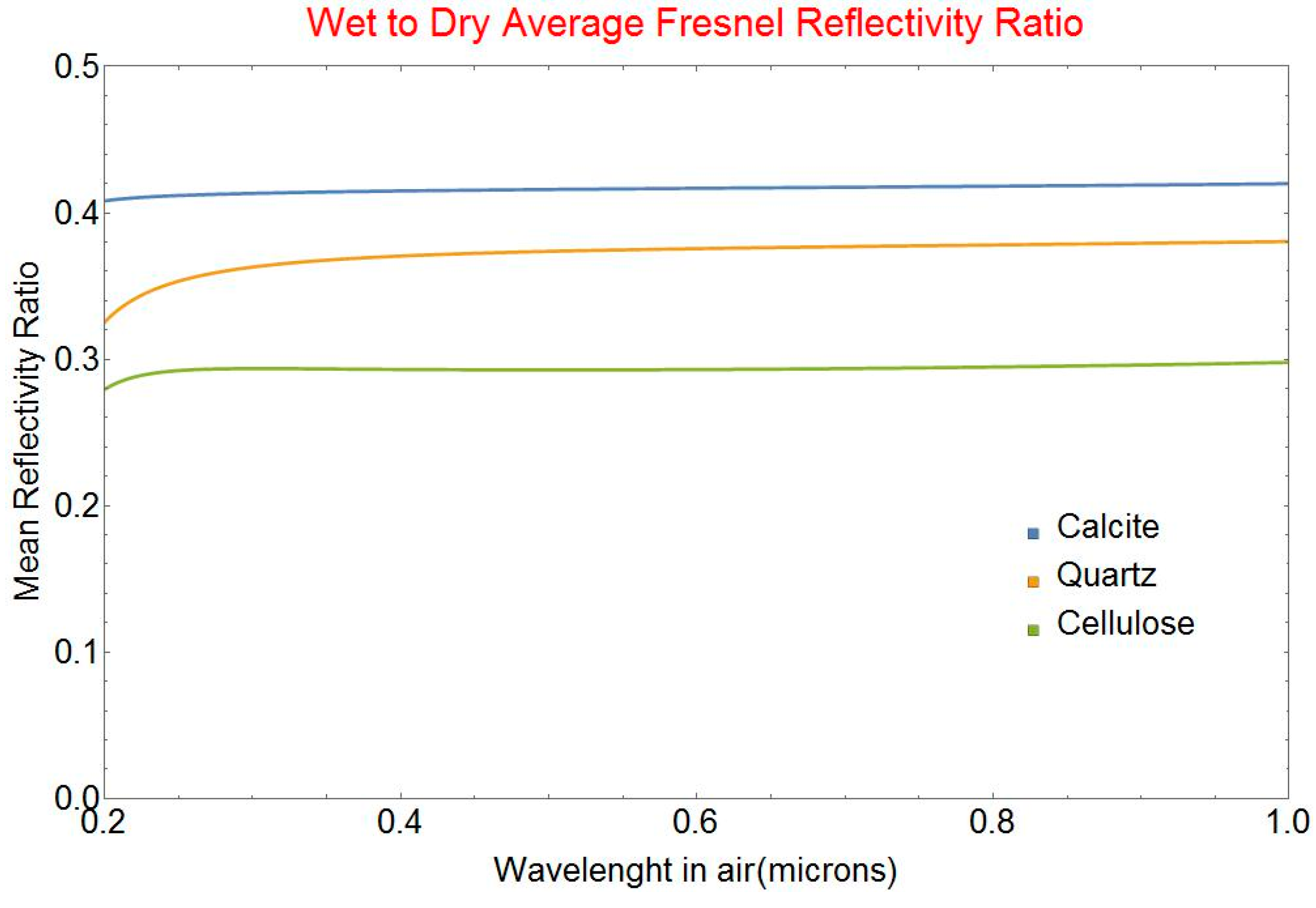
2.2. Dry to Wet Reflectance Ratio

Note that the wavelength dependence of the backscattering coefficient is a direct consequence of the wavelength dependence of the relative index of refraction. One important consequence of this dependence on the relative index of refraction is the reduction in $b_b\left(\lambda \right)$ when the interfaces between the grains are filled with water instead of air. This effect is the source of the lowering of the irradiance reflectance of materials and vegetation immersed in water. Because the interstitial gaps are small the grain structure and spacing $\langle d\rangle$ is the same in both cases, we can estimate the water to air ratio directly.

$$\frac{b_{bw}\left(\lambda \right)}{b_b\left(\lambda \right)}=\frac{{\omega }_t\left(n/n_w\right)}{{\omega }_t\left(n\right)},$$

(13)

Since the absorption does not change, we can directly estimate the ratio of backscattering albedo.

$$\frac{x_{bw}\left(\lambda \right)}{x_{ba}\left(\lambda \right)}=\frac{\frac{a\left(\lambda \right)}{b_b\left(\lambda \right)}+1}{\left[\frac{{\omega }_t\left(n\right)}{{\omega }_t\left(n/n_w\right)}\right]\frac{a\left(\lambda \right)}{b_b\left(\lambda \right)}+1},$$

(14)

$x_{bw}\left(\lambda \right)$ is the backscattering albedo in water while $x_{ba}\left(\lambda \right)$ is the corresponding backscattering albedo in air.

We can at this time estimate the wet to dry reflectivity factors for three of the most important and frequently found components of materials and vegetation, crystalline quartz, calcite and cellulose.

These are shown in Figure 2. The detailed formulas as a function of wavelength for these important indices are given in Appendix A. These indices can be found in references [11,12,13,14,15].

2.3. Basic Irradiance Reflectance Model

To estimate the irradiance reflectance from the backscattering albedo we use the Albert and Mobley algebraic radiance model valid for the infinitely deep medium case. The model is based on a careful analysis of solutions of the radiative transfer equation by the Hydrolight code for over 177,000 cases that encompass the full range of parameters for optically complex waters [1].

$$R_{\infty }=p_{1}x\left(1+p_{2}x+p_3{x}^2+p_4{x}^3\right)\left(1+p_5\frac{1}{\cos {\theta }_s}\right),$$

(15)

In this formula $R_{\infty }$ is the irradiance reflectance over waters deep enough that there is no contribution from the bottom reflectance. ${\theta }_s$ is the sun angle just below the surface of the scattering medium. Standard irradiance reflectance measurements are carried out by comparing the signal from a high-quality diffuse reflecting surface (Spectralon) that fills the field of view of the portable spectrometer to the signal from the substance to be measured under the same illumination conditions. Therefore, we must normalize the original Albert and Mobley expression to have $R_{\infty }=1$ when $x=1$.

$$R_{spc-\infty }=\frac{p_{1}x\left(1+p_{2}x+p_3{x}^2+p_4{x}^3\right)}{p_1\left(1+p_2+p_3+p_4\right)},$$

(16)

We have used the notation $R_{spc-\infty }$ in Equation (16) to clearly note that we are referring to the calibrated Spectralon normalized irradiance reflectance but from now on we will simply assume that all reflectances have been properly normalized.

Table 2. Coefficients of the Albert-Mobley model for the infinite medium depth case.

Coefficient	${\mathit{R}}_{\mathit{\infty }}$
$p_1$	0.1034
$p_2$	3.3586
$p_3$	−6.5358
$p_4$	4.6638
$p_5$	2.4121

gives the coefficients of Equations (15) and (16).

The expression that Albert and Mobley use is based on an extensive empirical survey carried out with an exact radiative code. The results of this survey are fitted as a fourth order polynomial which is an inconvenient form to use if we need in some cases to reverse the process and, for instance, estimate $x$ from $R_{spc-\infty }$. Aas [5] developed a two-stream radiative model and obtained approximate solutions for the irradiance reflectance from an infinite depth medium. We found that we could closely match the result of Albert and Mobley by parametrizing the formulas given by Aas. This approach yields simpler more general formulas that can easily be inverted as desired.

$$R_{spc-\infty }=\frac{\left(1+f^2\right)-\sqrt{{\left(1+f^2\right)}^2-4f^2{x}^2}}{2f^{2}x},$$

(17)

$f$ is an empirical parameter that varies from 0 to 1. A very close fit to the results of Albert and Mobley is obtained with $=0.79$. We have used the notation $R_{spc-\infty }$ in Equations (16) and (17) to clearly note that we are referring to the calibrated Spectralon normalized irradiance reflectance but from now on we will simply assume that all reflectance have been properly normalized to unity. Formula (17) is easily inverted to obtain $x$ as a function of $R$ if required.

$$x=\left(\frac{1+f^2}{f}\right)\left(\frac{fR}{1+f{R}^2}\right),$$

(18)

The value of $f$ is correlated with but not equal to the mean cosine of the total scattering function $\langle \cos \rangle$ which is defined as follows.

$$\langle \cos \rangle =2\pi \underset{0}{\overset{\pi }{\int }}p\left(\theta ,\lambda \right)\cos \theta \sin \theta d\theta ,$$

(19)

when $f=0$, the single scattering is nearly isotropic and the irradiance reflectance is equal to the backscattering albedo. When $f$ approaches 1 the single scattering becomes highly forward peaked. Note that $p\left(\theta ,\lambda \right)$ is the total scattering function and it includes both the reflected and the transmitted part of the radiation. The transmitted part is controlled by refraction and diffraction which dominate scattering in the forward hemisphere for grains or cells much larger that the wavelength. In the cases that concern us in this work the grains or cells are large enough that the transmitted part controls the value of the mean cosine.

2.4. Irradiance Reflectance Model for Translucent Subtances

There is one more common case we have to concern ourselves with: translucent organic materials growing on a mineral substrate. In order to model this situation we use the irradiance reflection model for finite bottom depth of Albert and Mobley [1]. The irradiance reflectance of the underlying material is used as a bottom irradiance reflectance $R_b$ in this case. The irradiance reflectance of the combination of translucent overlay of reflectance $R_{\infty }$ and thickness $z_b$ with a substrate of reflectance $R_b$ is modeled by the following equations.

$$R_t=R_{\infty }\left[1-A_1{e}^{-\gamma \left(\lambda \right)z_b}\right]+R_b{A}_2{e}^{-\delta \left(\lambda \right)z_b},$$

(20)

with:

$$\delta \left(\lambda \right)=\left[{\kappa }_0+{\left(1+x\left(\lambda \right)\right)}^{{\kappa }_{1w}}\left(1+{\kappa }_{2w}\right)\right]\left(\frac{b_b\left(\lambda \right)}{x\left(\lambda \right)}\right),$$

(21)

$$\gamma \left(\lambda \right)=\left[{\kappa }_0+{\left(1+x\left(\lambda \right)\right)}^{{\kappa }_{1b}}\left(1+{\kappa }_{2b}\right)\right]\left(\frac{b_b\left(\lambda \right)}{x\left(\lambda \right)}\right),$$

(22)

Table 3. Coefficients of the Albert-Mobley model for the finite medium depth case.

Coefficient	${\mathit{R}}_{\mathit{\infty }}$
$A_1$	1.0000
${\kappa }_0$	1.0546
${\kappa }_{1W}$	1.9991
${\kappa }_{2W}$	0.2995
$A_2$	1.0000
${\kappa }_{1b}$	1.2441
${\kappa }_{2b}$	0.5182

gives the coefficients of Equations (20)–(22).

The new parameter that controls the behavior of the combined solution is $u_b=b_b\left(\lambda \right)z_b$. Assuming the overlaying vegetation completely covers the substrate then, as the thickness of the overlay $z_b$ increases, the combined reflectance $R_t$ goes to the reflectance of the overlay $R_{\infty }$ while when $z_b$ becomes small the combined reflectance approaches $R_b$ as expected. What the model above shows is that the usual approach of linearly combining the separate reflectance signatures of the mineral substrate and the organic cover according to the weights of their relative areas only works in the limit where the cover is thick enough. For thin organic covers there is an exponential transfer of signature from substrate to cover which is a strong function of wavelength through the backscattering albedo of the translucent overlay $x\left(\lambda \right)$.

3. Results

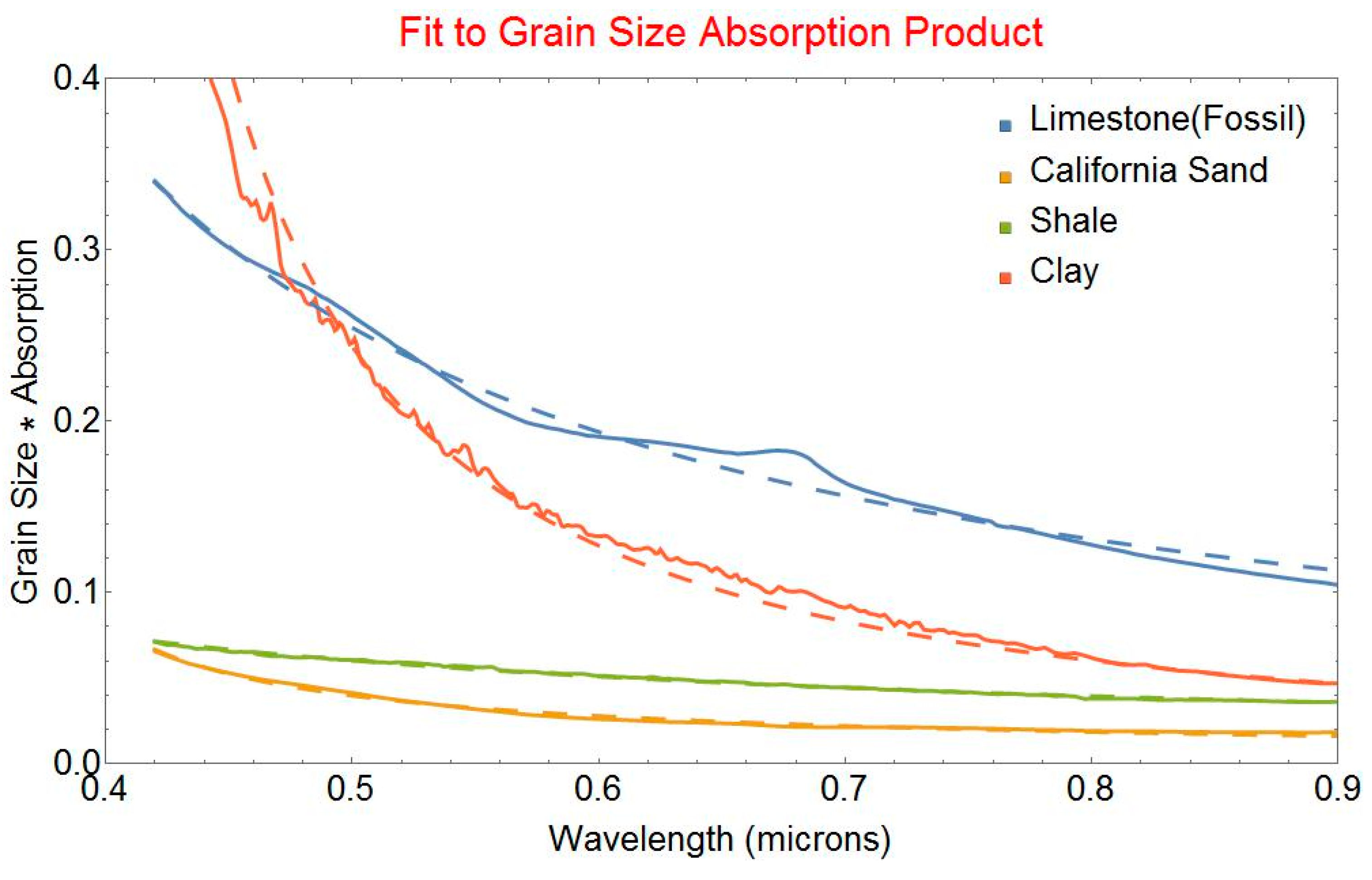
3.1. Specific Properties of Minerals

As mentioned briefly in the introduction, in the near-UV and visible the reflectance from mineral compounds is predominantly due to absorption and backscattering in the bulk material. For minerals this absorption comes from the broadened far wing of the lowest energy electronic transitions in the deep UV [2,3,4] and the backscattering is dominated by reflections at the interface between the crystalline grains of the material. The usual method for obtaining the absorption spectrum of mineral compounds is to measure the transmission loss through a sample of known thickness made from mineral powder that has been pressed and sintered. This is a time-consuming process that requires great care to obtain sufficiently low backscatter. Using our model opens up the possibility of obtaining the relative absorption spectra in the visible near-infrared (IR) region by simply measuring their irradiance reflectance.

Given the irradiance reflectance $R$ we first obtain the backscattering albedo $x$ from Equation (18). Using the definition of the backscattering albedo (1) and the Formula (5) we derived for $b_b\left(\lambda \right)$ we obtain the following expression for the absorption spectrum:

$$\langle d\rangle a\left(\lambda \right)=\frac{5}{6}{\omega }_t\left(n\right)\frac{\left(1-x\right)}{x},$$

(23)

Except for the scale factor of the mean crystalline grain size $\langle d\rangle$ we can now directly obtain the absorption spectrum for any substance for which we have measured an irradiance reflectance. We will use a simple approximate empirical functional form for the far wing absorption spectrum of an electronic transition which includes the cases of broadening due to internal collision and Van der Wall like interactions in the bulk of the material.

$$\langle d\rangle a\left(\lambda \right)=\frac{{\alpha }_o}{{\left(\lambda -{\lambda }_o\right)}^{\nu }},$$

(24)

Note that there is still a considerable amount of physical meaning to the parameters in the formula above. ${\lambda }_o$ is an estimate of the central wavelength of the lowest energy electronic transition. The value of $\nu$ is a function of the shape of the interaction potential of the molecular components of the crystalline grain. In the limiting case of an abrupt delta function like interaction potential $\nu =2$ and Equation (24) becomes a far wing Lorentzian profile [4] which is the standard abrupt collison lineshape. In the case of a sample of Trenton Limestone measured on the shore of Lake Ontario we obtain a very good fit of $\langle d\rangle a\left(\lambda \right)$ using the $\nu =1$ solution. This solution is indicative of a smoothly varying interaction potential similar to that of a linear spring.

$$\langle d\rangle a\left(\lambda \right)=\frac{0.081}{\left(\lambda -0.183\right)},$$

(25)

Many other values of $\nu$ are obviously possible and depend on the form of the interaction potential. Using expression (25) we can reconstruct the reflectance spectrum. Figure 3 shows a graph of the fit between the original reflectance and the one computed using our formulas.

The fits are quite accurate over the visible spectrum from 0.35 to 0.90 micron and we expect similar accuracy for materials whose absorption is not dominated by inclusions containing color centers. The results presented in

Table 4. This is a table of the functional fits to various minerals according to the formula.

Substance	${\mathit{a}}_{\mathit{o}}$	$\mathit{\nu }$	${\mathit{\lambda }}_{\mathit{o}}$	${\mathit{\sigma }}_{\mathit{r}}\left(\mathit{\%}\right)$
California Sand	0.01055	0.708	0.346	5.0
Hawaii Sand	0.04631	1.438	0.102	4.8
Greenland Sand	0.03323	0.453	0.350	4.9
Limestone (Trenton)	0.08401	1.217	0.102	3.8
Limestone (Fossil)	0.01662	0.688	0.348	6.6
Clay	0.02180	1.273	0.350	5.9
Sandy Loam	0.01087	1.882	0.195	4.1
Gray Silty Loam	0.00850	1.636	0.298	3.3
Brown Loam	0.01292	1.595	0.286	3.4
Dark Loam	0.02345	1.395	0.350	4.5
Granite	0.02102	0.737	0.304	8.6
Schist	0.11558	0.134	0.338	0.9
Shale	0.02988	0.738	0.113	1.5
Shale	0.04426	1.165	0.101	6.5
Shale	0.02364	0.219	0.344	2.8
Shale	0.11558	0.368	0.350	3.3
Siltstone	0.02669	0.229	0.345	3.9
Siltstone	0.01803	0.377	0.343	4.2

demonstrate that this is indeed the case.

Table 4 is the result of the fit for a set of materials of interest that could possibly be found on the bottom of the water column. The fit was constrained to a region from 0.42 to 0.90 microns. This wavelength zone was chosen to avoid the reflectance measurement accuracy problems that notoriously plague the near-UV and deep blue region of the spectrum. The standard deviation of the relative error in percent between the model and the data ${\sigma }_r(\%)$ is given in the last column.

The low standard deviation of the relative error shows that the fits are very close and are in several cases within the instrumental reflectance measurement variation. Formula (24) can, therefore, serve to fit experimentally measured reflectances. We originally hoped that in the limit, the values of the parameters ${\lambda }_o,\nu$ and ${\alpha }_o$ could even be used as markers to identify an unknown material. The results given in Table 3 are not encouraging in this respect as there is a great deal of variability even for similar materials. The situation is, however, not hopeless as we have noted that several of the signatures are affected by the presence of absorbtion by organic compounds and by the colour centers of mineral inclusions. Whether these effects can be properly adressed will require further studies. We begin to address the problem of the presence vegetation in the following sections.

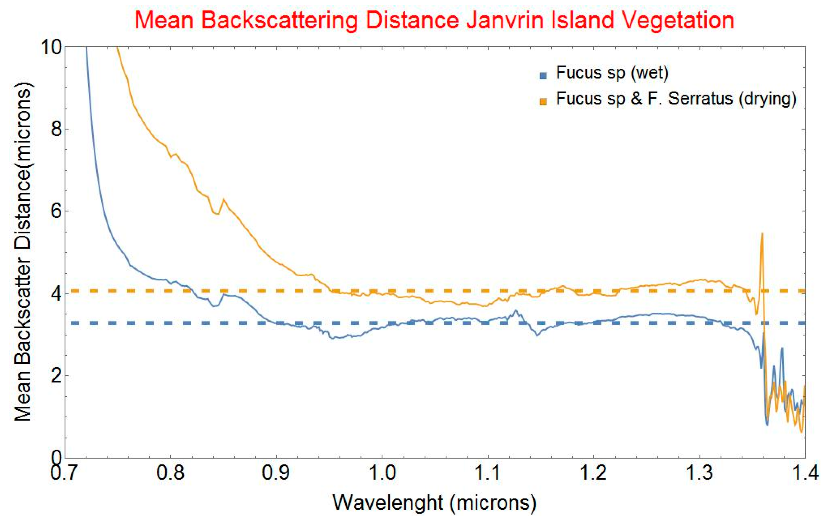
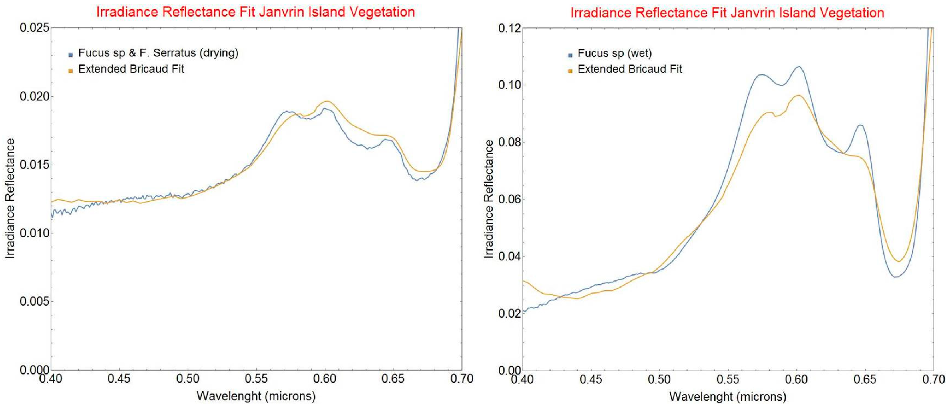
3.2. Specific Properties of Vegetation

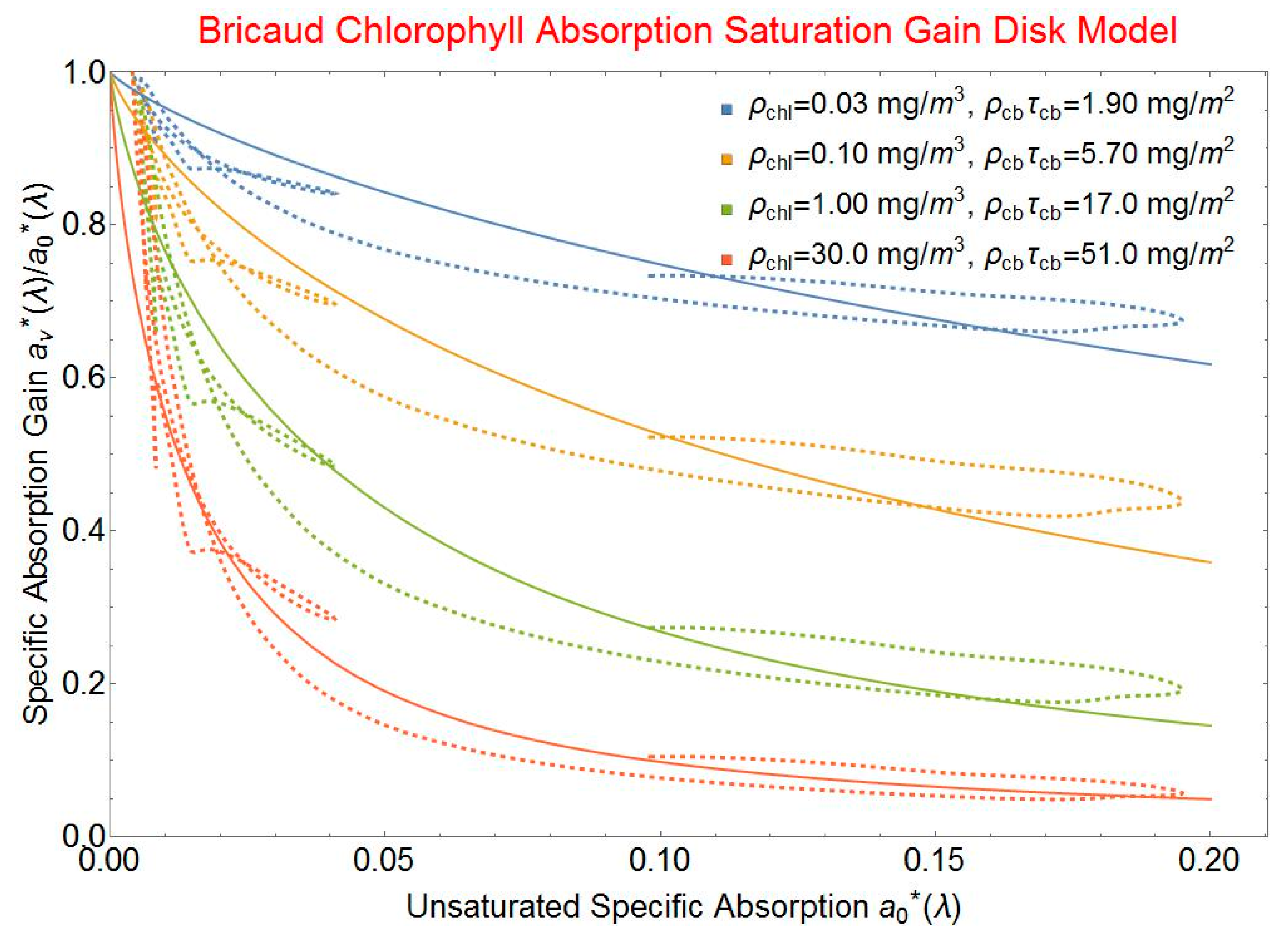
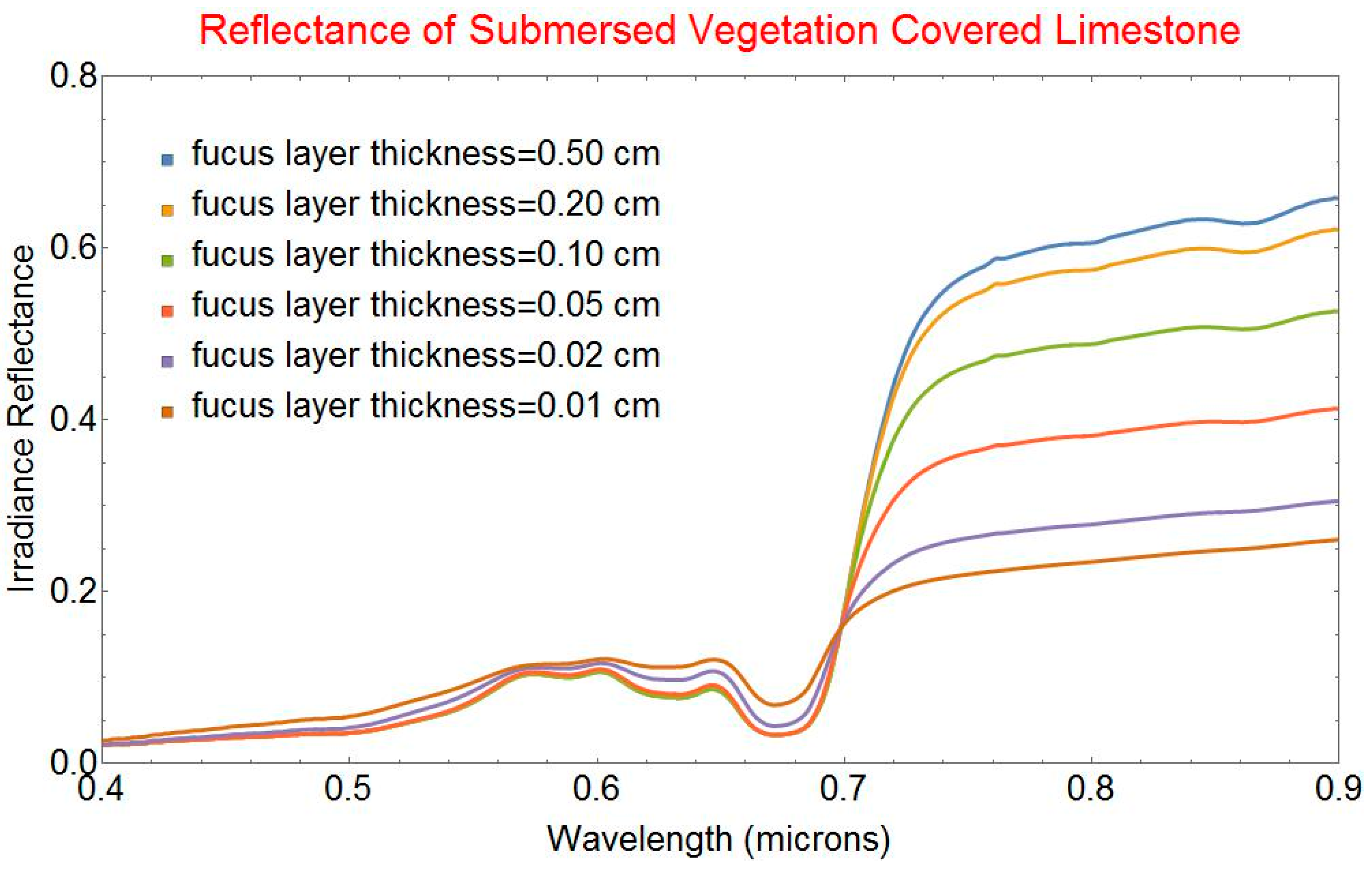
Absorption in vegetation is controlled by the absorption of the chlorophyll-a filled chloroplasts in the cell. As the concentration of chlorophyll-a and/or the size of the chloroplasts increases the absorption through the cell increases until the chloroplast absorbs more of the light at a given wavelength until in the limit of large concentrations and/or size it becomes a dark spot masking all the light its surface intercepts at this wavelength. This absorption saturation effect was first extensively studied by Morel and Bricaud [8] who called it the package effect. This is the factor that dominantes the variability in the absorption spectrum for different types of vegetation.

To compute this effect first we need formulas for the absorption efficiency $Q_a$ of the chloroplasts. These are derived in Appendix B for both the original model that asssumed a spherical shape for the chloroplasts and for a new model that assumes disk-like chloroplasts.

As mentioned in Appendix B, the exact formulas can be approximated to a sufficent accuracy by a simpler exponential model. From now on we will use the more realistic disk-like shape to model the absorption saturation effect.

$$a_v^{\ast }\left(\lambda \right)=\left(\frac{1}{2u_{cp}}\right)\left(1-e^{-a_o^{\ast }\left(\lambda \right)2u_{cp}}\right),$$

(26)

With:

$$u_{cp}={\rho }_{cp}{\tau }_{cp},$$

(27)

$a_o^{\ast }\left(\lambda \right)$ is the specific mass absorption coefficient of chlorophyll-a at low concentration in units of m² gr⁻¹. ${\rho }_{cp}$ is the chlorophyll-a mass density inside the chloroplast in gr m⁻³ and ${\tau }_{cp}$ is the thickness of the chloroplast disk in meters. The mean thickness of a randomly oriented set of disks is $2{\tau }_{cp}$ which explains the factor of 2 seen in Equation (26).

We verified the validity of this model by first comparing the theory for disks given by Equation (26) with the Bricaud et al. [9] empirical formula for chlorophyll-a absorption in type I waters which is based on in-depth analysis of a compilation of most of the available datasets. To do this we rewrite Equation (26) as a specific absorption gain function:

$$\frac{a_v^{\ast }\left(\lambda \right)}{a_o^{\ast }\left(\lambda \right)}=\left(\frac{1}{a_o^{\ast }\left(\lambda \right)2u_{cp}}\right)\left(1-e^{-a_o^{\ast }\left(\lambda \right)2u_{cp}}\right),$$

(28)

As can be seen in Figure 4, the overall behavior of the absorption is captured by the gain formula and this over three orders of magnitude in chlorophyll-a density. We note that the hysteresis seen in the empirical curves is due to an additional wavelength shift as a function of chlorophyll-a density. This effect was in fact observed by Gitelson [16]. The results shown in Figure 4 are a strong indication that the dominant effect in the spectral variation as a function of chlorophyll-a density is the absorption saturation effect. There was a large amount of variability in the original experimental data sets on which the empirical formulas are based so the discrepancies are not surprising. However, in the case that concerns us, which is the absorption in vegetation itself, the number density of phytoplankton which is the main uncontrolled empirical variable becomes severely constrained. The bulk chlorophyll-a mass density ${\rho }_{chl}$ is given by:

$${\rho }_{chl}=n_c{n}_{cp}{\rho }_{cp}{V}_{cp},$$

(29)

The number density of cells is $n_c$, the number of chloroplasts per cell is $n_{cp}$ and the volume of each chloroplast is $V_{cp}$. In the open ocean, $n_c$ may be weakly correlated with the other parameters while in a continuous block of cells as is the case in vegetation there is a very strongly constrained relationship. We can see this as follows. For a volume of vegetation $V_m$ filled by cells with a volume $V_c$ we have:

$${\rho }_{chl}{V}_m=\left(\frac{V_m}{V_c}\right){\rho }_{cp}{n}_{cp}{V}_{cp}=V_m{\rho }_{cp}\left(\frac{n_{cp}{V}_{cp}}{V_c}\right),$$

(30)

$${\rho }_{chl}={\rho }_{cp}\left(\frac{n_{cp}{V}_{cp}}{V_c}\right),$$

(31)

We expect the ratio of the total volume of chloroplasts $n_{cp}{V}_{cp}$ to the cell volume $V_c$ to be almost constant. The variability induced by $n_c$ for open water has disappeared and the bulk chlorophyll-a concentration is now as expected simply proportional to the chlorophyll-a concentration inside the chloroplasts that we use to estimate the absorption saturation.

The main implication of the discussion above is that we expect to be able to model the spectral shape of the absorption spectrum of chlorophyll-a with a single fitting parameter $u_{cp}$. Before this becomes feasible, there are, however, several significant hurdles which have to be overcome. First, the Bricaud formula for chlorophyll-a absorption can be scaled to any concentration no matter how small even for ranges that lie well outside the zone of the data used for the original fit. This creates a problem when trying to determine $a_o^{\ast }\left(\lambda \right)$ as a limiting value for low chlorophyll-a concentrations as we can extrapolate back to unphysically small values of concentration. Ciotti et al. [10] used a different approach to model the chlorophyll-a absorption from naturally occurring populations of organisms. They determine the absorption spectra for two limiting populations of organisms, the nano population and micro population. For low concentrations of chlorophyll-a the absorption spectrum of the nano population applies while for high concentrations the spectrum of the micro population is the appropriate one to use. As the concentration of chlorophyll-a increases, the spectrum evolves as a linear combination of both these extreme cases. We first attempted to use the nano population spectrum from Ciotti et al. [10] as the limiting case $a_o^{\ast }\left(\lambda \right)$ for low chlorophyll-a concentrations. Unsurprisingly, we found that the difference between our model and the Bricaud form diverged significantly at the higher concentrations.

This is problematic since for vegetation, which is the case of interest for us, the chlorophyll-a concentrations are expected to be large. In fact, they exceed the range of validity of the Bricaud formulas. To handle these extreme cases with a reasonable expectation of accuracy we decided to take a different approach. The technique is based on using a Bricaud spectrum at a given reference value with sufficiently high chlorophyll-a concentration but in a zone where the fit is still valid and extending the range from that point using the gain saturation equations. The rationale to do this is based on the fact that the concentration exceeds the measurement range and until data is available there is no other valid approach. This extension method proceeds as follows. Defining $u_r$ as the value of $u_{cp}$ at a reference bulk concentration ${\rho }_r$ we have:

$$a_r^{\ast }\left(\lambda \right)2u_r=\left(1-e^{-a_o\left(\lambda \right)2u_r}\right),$$

(32)

$$a_o\left(\lambda \right)2u_r=\ln \left[1/\left(1-a_r^{\ast }\left(\lambda \right)2u_r\right)\right],$$

(33)

$$a_o\left(\lambda \right)=\left(\frac{1}{2u_r}\right)\ln \left[1/\left(1-a_r^{\ast }\left(\lambda \right)2u_r\right)\right],$$

(34)

This $a_o\left(\lambda \right)$ is completely determined by the reference spectrum $a_r^{\ast }\left(\lambda \right)$ and the value we choose for $u_r$. Note that for $a_o\left(\lambda \right)$ to stay finite at all wavelengths there is a maximum value that $u_r$ can take:

$$\max u_r=\left(\frac{1}{\max \left[2a_r^{\ast }\left(\lambda \right)\right]}\right),$$

(35)

Using (34) we can write that:

$$a_o\left(\lambda \right)2u_{cp}=\left(\frac{u_{cp}}{u_r}\right)\ln \left[1/\left(1-a_r^{\ast }\left(\lambda \right)2u_r\right)\right],$$

(36)

Finally, we obtain the following general expression for an extended Bricaud absorption spectrum that can be used at chlorophyll-a densities appropriate for vegetation:

$$a^{\ast }\left(\lambda \right)=\left(\frac{1}{2u_{cp}}\right)\left(1-e^{-a_o\left(\lambda \right)2u_{cp}}\right),$$

(37)

As a final practical step we need to determine what value of ${\rho }_r$ we will use a reference spectrum and what value of $u_r$ leads to the most reliable extrapolation. To do this we first choose the Bricaud spectrum for 5.0 mg/m³ which is a value at the high end of the bulk concentration range but still well below the 20.0 mg/m³ extreme limit of the data on which the formula was based. To determine the best value of $u_r$ we varied that parameter until we obtained the best fit to the Bricaud spectra at 1.0, 3.0 and 10.0 mg/m³. In all these cases we found that the optimum reference $u_r$ asymptotically approached $\max u_r\left(\lambda \right)$. In practice, therefore, we recommend using a value of 0.99 $\max u_r\left(\lambda \right)$.

To completely model the absorption due to vegetation we need to include the absorption of water and of the cellulose that makes up the walls and internal structures of the cell. The absorption spectrum of water is taken from the data of Pope and Fry [17] for the zone from 0.38 to 0.70 microns and from the data of Kou [18] normalized to the data of Pope and Fry in their wavelength overlap zone for the 0.65 to 2.5 microns range.

The specific absorption spectrum of naturally occurring lignin cellulose from 0.4 to 2.5 microns is given in [19]. The spectrum of crystalline cellulose from 0.2 to 0.5 micron in arbitrary units can be found in reference [20]. We used the overlap zone from 0.4 to 0.5 microns with the calibrated spectrum in [16] to transform the UV-visible spectrum given in [20] to specific absorption in units of m²·gr⁻¹. We will use the pure water, chlorophyll-a and cellulose absorption spectra to model the irradiance reflectance spectra of algae and other marine vegetation.

3.3. Modeling Algae

We are now in a position to analyse the spectral signature of algae and other marine vegetation. The spectra we will be using were collected on the shores of Janvrin Island in Nova Scotia. These calibrated reflectance spectra range from 0.35 to 2.5 microns. This range extends beyond the wavelength band over which chlorophyll-a absorption has a significant amplitude. This is fortunate in as much as we can use the reflectance measured in the wavelength range over 0.90 micron to obtain a measurement of $\langle d\rangle$. This is because the components which dominate absorption in that wavelength range are water and cellulose and their absolute values and relative abundances are well known. In that spectral band, therefore, we have:

$$\langle d\rangle =\left(\frac{1-x\left(\lambda \right)}{x\left(\lambda \right)}\right)\frac{{\omega }_b\left(n_{cw}/n_w\right)}{\left[a_w\left(\lambda \right)\left(1-f_{cl}\right)+f_{cl}{a}_{cl}\left(\lambda \right)\right]},$$

(38)

$f_{cl}$ is the mass fraction of cellulose in the cell and $n_{cw}$ is the index of refaction of the walls of the cell and its subcomponents and $n_w$ is the index of refraction of water. This cell wall index has been estimated for both the mesophyll and antidermal cell walls by Baranoski [12]. Since both are quite close to one another we use their average value as an estimate for $n_{cw}$.

We can use the fact that the mean spacing between backscattering layers $\langle d\rangle$ should be independent of wavelength to estimate $f_{cl}$. To do this, we vary $f_{cl}$ to minimize the variance in the estimate of $\langle d\rangle$ as a function of wavelength computed with Equation (39). We use the wavelength range from 0.90 to 1.35 micron. We need to be above 0.90 microns to ensure that we are completely out of the zone where there could be remaining absorption by chlorophyll-a and other pigments in the algae. We also must stay below 1.35 micron to remain below the large water absorption band which reduces the irradiance signal to levels where instrument noise totally dominates. Figure 5 and

Table 5. Functional fits to the mean spacing of backscatter layers $\langle d\rangle$.

Substance	${\mathit{f}}_{\mathit{c}\mathit{l}}$	$\langle \mathit{d}\rangle \left(\mathit{m}\mathit{i}\mathit{c}\mathit{r}\mathit{o}\mathit{n}\mathit{s}\right)$	${\mathit{\sigma }}_{\langle \mathit{d}\rangle }$	${\mathit{\sigma }}_{\langle \mathit{d}\rangle }/{\mathit{\mu }}_{\langle \mathit{d}\rangle }$
Fucus sp.	0.043	3.29	0.15	0.048
Fucus sp. & F. serratus	0.164	4.07	0.21	0.054

show the result of such a fit to the reflectance spectra of wet Fucus sp. and a drying mixture of Fucus sp. and F. serratus from Janvrin Island in Nova Scotia. These samples were chosen because they represent the extreme values of the reflectance spectra we measured. The results show the potential of this approach to estimate the status of the vegetation. In this case the Fucus sp. is much more saturated with water than the drying mixture sample while the mean backscattering feature size of the mixture is larger. The ratio of the standard deviation to the mean value of $\langle d\rangle$ is of the order of 5% in both cases which shows that a constant mean value $\langle d\rangle$ is a good model for the data.

Once we have obtained the value of $\langle d\rangle$ we can use it in the wavelength range where the absorption of cholorophyll is dominant.

$$a_v\left(\lambda \right)={\rho }_{chl}{a}_v^{\ast }\left(\lambda \right)=\left(\frac{1}{\langle d\rangle }\right)\left(\frac{1-x\left(\lambda \right)}{x\left(\lambda \right)}\right){\omega }_b\left(n_{cw}/n_w\right)-\left[a_w\left(\lambda \right)\left(1-f_{cl}\right)+f_{cl}{a}_{cl}\left(\lambda \right)\right],$$

(39)

As a final step we can now estimate the absorption saturation parameter $u_{cp}$ and the bulk cholorophyll concentration ${\rho }_{chl}$ by using Equation (39) and performing a non-linear least squares fit on the ratio of the experimental absorption obtained with the procedure described above to the low chlorophyll-a concentration limit $a_o^{\ast }\left(\lambda \right)$.

$$\left(\frac{{\rho }_{chl}}{2u_{cp}}\right)\left(1-e^{-a_o^{\ast }\left(\lambda \right)2u_{cp}}\right)=\left(\frac{1}{\langle d\rangle }\right)\left(\frac{1-x\left(\lambda \right)}{x\left(\lambda \right)}\right){\omega }_b\left(n_{cl}/n_w\right)-\left[a_w\left(\lambda \right)\left(1-f_{cl}\right)+f_{cl}{a}_{cl}\left(\lambda \right)\right],$$

(40)

Figure 6 shows the result of such a fit for a reflectance spectrum of wet Fucus sp. and a drying mixture of Fucus sp. and F. serratus. Note the significant noise increase in the short wavelength region. This is due to the signal to noise of the reflectance measuring instrument in the blue and near UV. This significant spectral variation of the signal to noise forces us to use of an appropriate weighing function in performing the fit.

Once this weighing is applied we can see that the resulting modeled absorption spectrum approaches the experimental results.

In order to further verify the accuracy of the predictions of the model we have used the parameters of the fit to compute directly the predicted irradiance reflectance spectra and compare them to the original measured spectra. The results are shown in Figure 7 below.

The error between the modeled and measured reflectance signatures is of the same relative magnitude as the corresponding error in the absorption fit shown in Figure 6. Given the simplicity and generality of the model the overall precision of the fit is sufficient to satisfy our original purpose of hyperspectral bathymetry in uncharted waters.

One should note that the present model does not explicitely involve accessory pigments such as fucoxanthin which is known to be present in Fucus. It is based on the transformation due to absorption saturation in the chloroplasts (package effect) of the spectrum of phytoplankton. This phytoplankton spectrum is taken here as an archetype of a naturally occuring assemblage of various pigments dominated by chlorophyll-a. The absorption saturation effect shifts the resulting reflectance spectrum to the yellow and red which accounts for the relative closeness of the fit even without specific contributions from the accessory pigments. In the bathymetry application which most concerns us, the overall spectral shift and absolute level of the absorption are the key parameters needed to obtain reliable estimates of the depth. Given the exact pigment composition one could obviously improve the fit to the reflectance spectrum. However, this would defeat the purpose of obtaining the depth and the bottom spectrum without any a priori information other than the reflectance spectrum of the shoreline. This approach can, however, be improved by an iterative technique as we shall see in the discussion.

3.4. Non-Linear Effects of Vegetation Cover

We can now compute the effect of translucent vegetation growing over a mineral substrate. Because we have already obtained the mean cell size of the algae $\langle d\rangle$ we can directly compute its $b_b\left(\lambda \right)$ from Equation (5). This allows us to evaluate all the terms in Equation (16) and solve for the reflectance spectrum as a function of the actual thickness of the vegetation layer.

Figure 8 shows the variation in the spectral reflectance signature as a function of thickness for fucus over Trenton limestone. In the near IR, the spectra evolve from a high reflectance translucent signature for the pure Fucus to the low reflectivity of the wet limestone while in the visible zone that trend is reversed and the spectra go from the low reflectance of pure Fucus to the higher reflectance of wet limestone.

Note that in cases where we don’t have a separate estimate of $b_b\left(\lambda \right)$ we simply need to use directly the parameter $u_b=b_b\left(\lambda \right)z_b$. Given that we know the limiting spectra for the pure vegetation and for the mineral substrate $u_b$ is the only parameter required to define the reflectance spectrum of their combination.

4. Discussion

The simple model presented in the previous sections leads to several important insights into the behavior of the irradiance reflectance spectra of minerals and vegetation in the underwater environment. The first significant result is that we are now able to estimate the ratio of the reflectance of materials immersed in water to their dry state. Figure 9 shows the ratio of irradiance reflectance for limestone and for beach sand that can be computed using Equations (14) and (17) from our model.

The ability to transfer reflectance spectra measured in air to their in-water equivalent is of great importance in practice as there are many comprehensive sources of spectral signatures measured in air while very few data are available under water due to the obvious difficulties in measurement. These underwater reflectance spectra are the backbone of all near shore shallow water hyperspectral surveys and the accuracy of any depth or bottom cover composition depends directly on their estimates.

Using the algebraic radiative transfer model, we have shown that we can estimate directly from reflectance measurement the relative absorption spectrum $\langle \mathit{d}\rangle \mathit{a}\left(\mathit{\lambda }\right)$. Using these spectra, we have managed to obtain a simple and accurate fitting function whose structure is nevertheless based on fundamental physical considerations in far wing line broadening of the absorption from the lowest energy electronic transition in the material. Note that, strictly speaking, this fitting function is only appropriate for dielectric materials since the presence of the conduction bands in metals is not accounted for. The existence of this simple function valid over the range of wavelength of relevance to underwater hyperspectral measurements opens the possibility of identifying the material by a direct fit to the absorption parameters obtained from an inversion of the irradiance reflectance measurements of the water column using the algebraic radiative transfer model. The variance of the $\mathit{\nu }$ and ${\mathit{\lambda }}_{\mathit{o}}$ parameters seen in Table 4 which control the spectral shape of the material may be indicative of a fundamental difficulty in obtaining directly bottom-type identification from the measured airborne hyperspectral reflectance. Addressing the scope and precise nature of this problem will be the subject of a further study.

We have also obtained a similarly simple four-parameter fitting function to the reflectance spectra of vegetation. The first parameter is the mean size of the vegetative cells $\langle \mathit{d}\rangle$, the second parameter is the chlorophyll-a absorption saturation factor ${\mathit{u}}_{\mathit{c}\mathit{p}}$, the third parameter is the mass fraction of cellulose contained in a cell ${\mathit{f}}_{\mathit{c}\mathit{l}}$, and the fourth parameter is the bulk chlorophyll-a mass concentration ${\mathit{\rho }}_{\mathit{c}\mathit{h}\mathit{l}}$. The backscattering term is controlled by the relative index of cellulose in water and the mean size of the cells while the absorption is the weighed sum of the absorption of water, cellulose and chlorophyll-a. The cell absorption is composed the absorption of pure water, cellulose and chlorophyll-a. The shape of the absorption of chlorophyll-a is controlled by the package effect through the absorption saturation parameter ${\mathit{u}}_{\mathit{c}\mathit{p}}$ and its magnitude is controlled by the chlorophyll-a bulk density ${\mathit{\rho }}_{\mathit{c}\mathit{h}\mathit{l}}$. The parameters of the model are interrelated. Relationships such as the one given in Equation (27) open up the possibility of obtaining estimates of parameters such as the ratio of the total volume of the chloroplasts to the total cell volume which could be used as an indicator of cell health.

We have shown that the reflectance of a mix of vegetation and minerals is not just a simple relative area coverage problem. When vegetation grows on top of a mineral substrate there results a combined spectrum which depends in a highly non-linear fashion on the product of thickness of the vegetation times its backscattering coefficient ${\mathit{u}}_{\mathit{b}}$. The overall effect for the reflectance spectra ${\mathit{R}}_{\mathit{m}}\left(\mathit{\lambda }\right)$ of pixels which are partially covered in vegetation is a combination of this non-linear mixing and area coverage factor.

$$R_m\left(\lambda \right)=\left[R_b\left(\lambda \right)\left(1-f_{vp}\right)+f_{vp}{R}_t\left(\lambda \right)\right],$$

(41)

${\mathit{f}}_{\mathit{v}\mathit{p}}$ is the fractional per pixel vegetation cover. Given that the vegetation is generally expected to be of the same type and in substantially the same state of health over areas larger than a pixel it will in many cases be possible to separate the area coverage factor ${\mathit{f}}_{\mathit{v}\mathit{p}}$ from the backscattering thickness factor ${\mathit{u}}_{\mathit{b}}$. This new information has the potential to increase significantly the level of knowledge about the ecologically relevant status and distribution of the near shore underwater vegetation.

In summary, the model we proposed here helps limit the number of parameters that need to be fitted for an analysis of the marine environment with hyperspectral irradiance reflectance spectra. This is an important factor because of the restricted wavelength band available when working in the underwater environment. The added complexity of the overlying water column absorption and scattering spectrum renders extremely difficult and unstable any inversion directly based on fitting linear combinations of bottom reflectance spectra. The low reflectance values and the low signal-to-noise ratios as depth increases severely affect the detectable level of spectral variation. The spectral angle is often near or within the noise band so the only hope for reasonable depth and type of bottom estimates and identifications are to use general parameters in low numbers. This is the case with our model. Furthermore, all the parameters in the model have a physical basis and are amenable to being further constrained in their fitting range by any information available from other sources such as the size and shape of chloroplasts, size of mineral grains and size of the spacing for near-surface fragmentation and porosity of rocks and sand.

We are currently using as a default reference the specific absorption spectrum of Bricaud et al. [9]. Given the extensive work in relation to coral reefs on the end member spectra and their variability [21] it may be possible in future to derive reference spectra better suited to modeling vegetation that also include a better balanced and more comprehensive mix of accessory pigments. As we have seen, a substantial part of the vegetation reflectance signature differences and spectral variability may be explained by the choloroplast absorption saturation effect. The remaining differences could, therefore, be less significant than appear at first glance, thus potentially reducing the number of distinct spectral absorption compositions required to model the end member signatures set. The other potential contribution of the approach we have taken of modeling the reflectance signatures by a radiative transfer model is that the variability in the spectral signatures clearly outlined for instance by Hochberg et al. [21] can be related explicitly to several parameters of interest in the study of corals such as the thickness of the thin translucent organic cover $z_b$ over the mineral substrate (Equation (20)), the size of the scattering features of the cells, and their chloroplast pigment concentration.

We must remember that bathymetry in unknown waters is one of the main drivers for restricting the number of variables to optimize to obtain an estimate of the water column depth. The standard approach of using a combination of linear mixes is problematic when there is no ground truth or a priori knowledge of the bottom to restrict the space of end members for bottom reflectance. However, there is a way to use the best features of our model and the linear mixing method. We first solve for depth using the generic bottom reflectance model proposed here. Once the depth is estimated, we can use the measured water surface irradiance reflectance to derive the bottom spectrum that would produce that measured surface irradiance reflectance. Given this bottom spectrum we can then use the standard linear mixing method to determine the bottom vegetation and mineral types that compose it, thus extracting valuable information about the bottom type. Given this new information we can recompute the depth and correct for any error in the original approximate model, therefore maximizing the benefits of both approaches. This mixed method will be the subject of future investigations.

References

1. Albert, A.; Mobley, C. An analytical model for subsurface irradiance and remote sensing reflectance in deep and shallow case-2 waters. Opt. Express 2003, 11, 2873–2890. [Google Scholar] [CrossRef] [PubMed]
2. Jonasz, M.; Fournier, G. Light Scattering by Particles in Water: Theoretical and Experimental Foundations; Academic Press: New York, NY, USA, 2007; pp. 39–42, 77–80. ISBN 10: 0-12-388751-8. [Google Scholar]
3. Szudy, J.; Bayliss, W.E. Uniform Frank-Condon treatment of pressure broadening of spectral lines. J. Quant. Spectrosc. Radiat. Transf. 1975, 15, 641–668. [Google Scholar] [CrossRef]
4. Wooten, F. Optical Properties of Solids; Academic Press: New York, NY, USA, 1972; pp. 42–52. ISBN 9781483220765. [Google Scholar]
5. Aas, E. Two-stream irradiance model for deep waters. Appl. Opt. 1987, 26, 2095–2101. [Google Scholar] [PubMed]
6. Jonasz, M.; Fournier, G. Light Scattering by Particles in Water: Theoretical and Experimental Foundations; Academic Press: New York, NY, USA, 2007; pp. 119–120. ISBN 10: 0-12-388751-8. [Google Scholar]
7. Fournier, G.; Neukermans, G. An Analytical Model for Light Backscattering by Coccoliths and Coccospheres of Emiliania Huxleyi. Opt. Express 2017, 25, 14996–15009. [Google Scholar] [CrossRef] [PubMed]
8. Morel, A.; Bricaud, A. Theoretical results concerning light absorption in a discrete medium, and application to specific absorption of phytoplankton. Deep Sea Res. 1981, 28, 1375–1393. [Google Scholar] [CrossRef]
9. Bricaud, A.; Morel, A.; Babin, M.; Allali, K.; Claustre, H. Variations of light absorption by suspended particles with the chlorophyll-a a concentration in oceanic (Case 1) waters: Analysis and implications for bio-optical models. J. Geophy. Res. 1998, 103, 31033–31044. [Google Scholar] [CrossRef]
10. Ciotti, A.M.; Lewis, M.R.; Cullen, J.J. Assessment of the relationships between dominant cell size in natural phytoplankton communities and the spectral shape of the absorption coefficient. Limnol. Oceanogr. 2002, 47, 404–417. [Google Scholar] [CrossRef] [Green Version]
11. Ghosh, G. Dispersion-equation coefficients for the refractive index and birefringence of calcite and quartz crystals. Opt. Commun. 1999, 163, 95–102. [Google Scholar] [CrossRef]
12. Sultanova, N.; Kasarova, S.; Nikolov, I. Dispersion properties of optical polymers. Acta Phys. Pol. A 2009, 116, 585–587. [Google Scholar] [CrossRef]
13. Quan, X.; Fry, E.S. Empirical equation for the index of refraction of seawater. Appl. Opt. 1995, 34, 3477–3480. [Google Scholar] [CrossRef] [PubMed]
14. Schiebener, P.; Straub, J.; Levelt Sengers, J.M.H.; Gallagher, J.S. Refractive Index of Water and Steam as Function of Wavelength, Temperature and Density. J. Phys. Chem. Ref. Data 1990, 19, 677–717. [Google Scholar] [CrossRef]
15. Baranoski, G.V.G. Modeling the interaction of infrared radiation (750 to 2500 nm) with bifacial and unifacial plant leaves. Remote Sens. Environ. 2006, 100, 335–347. [Google Scholar] [CrossRef]
16. Gitelson, A. The peak near 700 nm on radiance spectra of algae and water: Relationship of its magnitude and position with chlorophyll-a concentration. Int. J. Remote Sens. 1992, 13, 3367–3373. [Google Scholar] [CrossRef]
17. Pope, R.M.; Fry, E.S. Absorption spectrum (380–700 nm) of pure water. II. Integrating cavity measurements. Appl. Opt. 1997, 36, 8710–8723. [Google Scholar]
18. Kou, L.; Labrie, D.; Chýlek, P. Refractive indices of water and ice the 0.65 to 2.5 m spectral range. Appl. Opt. 1993, 32, 3531–3540. [Google Scholar] [CrossRef] [PubMed]
19. Jacquemoud, S.; Ustin, S.L.; Verdebout, J.; Schmuck, J.; Andreoli, G.; Hosgood, B. Estimating leaf biochemistry using the PROSPECT leaf optical properties model. Remote Sens. Environ. 1996, 56, 194–202. [Google Scholar] [CrossRef]
20. Adolfo, A.; Martin, P.; UV-Visible NIR Microspectroscopy of Nanocrystalline cellulose. CRAIC Technol. 2013. Available online: http://www.warsash.com.au/news/articles/craic-application-paper.pdf (accessed on 10 May 2018).
21. Hochberg, E.J.; Atkinson, M.J.; Andrefouet, S. Spectral reflectance of coral reef bottom-types worldwide and implications for coral reef remote sensing. Remote Sens. Environ. 2003, 85, 159–173. [Google Scholar] [CrossRef]
Figure 1. This figure is a schematic of the microstructure elements relevant to scattering and absorption for both minerals (grains) and vegetation (cells). The incident light rays (1) are reflected (2) and transmitted at the first surface (3). The rays transmitted through the first surface are subsequently both reflected back from the inner surfaces of the grains (4) and absorbed. The rays that penetrate deeper (5) are multiply scattered before coming back to the surface and have a near Lambertian (uniform) scattering distribution.
Applsci 08 02680 g001
Figure 2. Wet to dry angularly averaged Fresnel reflectivity factors as a function of wavelength for important components of materials and vegetation: crystalline quartz, calcite and cellulose.
Applsci 08 02680 g002
Figure 3. Comparison of the dimensionless parameter grain size times absorption coefficient estimated using Formula (23) for various mineral compounds (solid lines) with the fit (dashed lines) obtained using Equation (25). The fit parameters are given in the corresponding entries of Table 4. The spectral features seen in the experimental reflectance of the Trenton limestone sample are due to an interstitial chlorophyll-a residue lying on top of the limestone.
Applsci 08 02680 g003
Figure 4. Graph of the ratio of the specific absorption gain to the unsaturated absorption gain. The dotted lines are from the empirical formula of Bricaud et al. [9] for chlorophyll-a. The solid lines are from Equation (21) with the parameters noted.
Applsci 08 02680 g004
Figure 5. Fit of the mean backscatter distance derived from the irradiance reflectance of wet Fucus sp. and a drying mixture of Fucus sp. and F. serratus from Janvrin Island in Nova Scotia. In the zone below 0.90 microns the absorption of the chlorophyll-a and various pigments starts to dominate while in the zone above 1.35 microns the absorption of water becomes large enough that the resulting irradiance reflectance signal is dominated by noise. The full parameters of the fit are given in Table 5.
Applsci 08 02680 g005
Figure 6. Fit of the absorption spectrum of wet Fucus sp. and a drying mixture of Fucus sp. and F. serratus with the extended Bricaud model. Note the noise due to the instrumental signal to noise degradation in the blue wavelength range. This effect was compensated by weighing the fit function inversely proportional to the S/N. The blue and yellow curves are the derived spectrum from the reflectance measurements and Equation (29). The green and red curves are the fit using Equation (37).
Applsci 08 02680 g006
Figure 7. Comparison of modeled irradiance reflectance spectrum of wet Fucus sp. and a drying mixture of Fucus sp. and F. serratus (yellow curves) with the experimental measurements (blue curves). Note the noise degradation of the instrumental signal in the blue wavelength range. This reduced sensitivity may explain part of the incipient discrepancy in that spectral region.
Applsci 08 02680 g007
Figure 8. Computed variation of the spectral signature of translucent fucus vegetation over Trenton limestone as a function of the thickness of the layer. The mean spacing between scattering surfaces d is 3.3 microns.
Applsci 08 02680 g008
Figure 9. Computed irradiance reflectance for wet limestone and beach sand. The spectral signature for dry limestone comes from the shore of Lake Ontario. The signature of dry sand comes from a beach in Santa Barbara.
Applsci 08 02680 g009