Use of Gradient-Based Shadow Detection for Estimating Environmental Illumination Distribution

Abstract

Environmental illumination information is necessary to achieve a consistent integration of virtual objects in a given image. In this paper, we present a gradient-based shadow detection method for estimating the environmental illumination distribution of a given scene, in which a three-dimensional (3-D) augmented reality (AR) marker, a cubic reference object of a known size, is employed. The geometric elements (the corners and sides) of the AR marker constitute the candidate’s shadow boundary; they are obtained on a flat surface according to the relationship between the camera and the candidate’s light sources. We can then extract the shadow regions by collecting the local features that support the candidate’s shadow boundary in the image. To further verify the shadows passed by the local features-based matching, we examine whether significant brightness changes occurred in the intersection region between the shadows. Our proposed method can reduce the unwanted effects caused by the threshold values during edge-based shadow detection, as well as those caused by the sampling position during point-based illumination estimation.

1. Introduction

Understanding the environmental illumination information of a scene is important when rendering virtual objects in a way that matches the given image; it particularly helps during the generation of convincing vertical shadows onto the real scene [1,2]. Without shadows, virtual objects will appear like they are floating, making the rendered image appear unrealistic. The goal of our study is to estimate the environmental illumination distribution and to improve the visual perception of an augmented reality (AR) system by generating virtual shadows.

Many studies have described the generation of realistic images that reflect the environmental illumination of their scene [3,4,5,6,7]. Some of these studies have employed additional camera equipment (e.g., a light probe or a fish-eye camera) to estimate real-world illumination conditions [8,9]. One previous study used mobile sensors (e.g., ambient sensors), a global positioning system (GPS), and a weather application programming interface (API) to estimate outdoor illumination for a mobile AR application [10].

Shadows are cast by the occluding object and the illumination source in a given scene, so they provide an important clue about the shape and the relative position of the object, as well as the environmental illumination. The shadow generated by a reference object with known geometry can therefore be examined to estimate the environment illumination [1,3,4]. However, the performance of point-based estimation methods is heavily dependent on the number of sampling points, and their positions of those points on the shadow’s surface. In addition, it is difficult to determine accurate threshold values with which to segment the shadow region. One study introduced an iterative voting scheme that compared inside-region (potential cast shadows region) pixels with outside-region pixels using shadow features [6]. In this method, the inside-region with respect to the three-dimensional (3-D) object was defined in an initial setup procedure, meaning that the dynamic situation in which the position of the illumination sources were changed was not considered. For example, when there is a wide distribution of illumination sources in the scene, the inside-region become too large. The illumination estimation performance is therefore significantly dependent on which point is sampled. However, the study did not present a detailed method for determining the sample points for iterative voting [6].

A further study introduced an illumination estimation method for a mobile AR system, under the assumption that there is a single dominant light source in the scene [3]. By jumping the shadow boundary trace along the current estimate of the shadow vector, this method was able to extract distinct contours from the shadowed region. As there are usually multiple light sources in real scenes, however, the shadow boundaries often have a complex distribution. In this case, the method adopted featured difficulties in tracing the exact shadow boundaries, even though several salient shadow edges were present in the scene [3].

Previous studies have extracted the shadow region and its boundary on a textured shadow surface in a static outdoor scene [5,11,12]. Also, the shadow detection is critical for accurate object detection in video streams since shadow points are often misclassified as object points, causing errors in segmentation and tracking [13,14,15]. However, these studies mainly examined shadow edges with distinct gradient distributions, because outdoor environments feature a main light source (sunlight). These methods were applied to a situation in which the sun was occluded, but they assumed that most of the shadow boundaries would still have large gradient magnitude values and distinct gradient directions. In general, it is difficult to detect precisely the shadow boundary by only using the image features.

One study constructed 3-D shape descriptions of buildings from the fragmented linear features in an aerial image [16]. The shadow lines cast by a roof and their shadow junctions were used to verify two-dimensional (2-D) building roof hypotheses. Here, the shadow boundaries were searched for among the lines and junctions extracted from the image. The method described the geometric information of the 3-D object, assuming that the sun angles and the viewpoint angles were known, starting with the line segments detected by a Canny edge detector. However, since shadow intensity is not generally uniform in real scenes, more consideration is needed to determine a proper threshold value for edge detection. The method of said study focused mainly on generating hypotheses of the linear features and verifying these hypotheses, but did not introduce a detailed description of linear feature detection and grouping. In addition, the sun was the only illumination source in the scene.

Our algorithm is inspired by the approach of Reference [16], in that we consider local shadow boundary features to be useful for extracting the shadow from the image. By generating the shadow using the candidate light source positioned on the hemisphere, we can obtain shadow-casting information for the boundary line segments and their junctions. We assume that the scene has a planar surface, on which the shadows are cast. The local supporting evidence (the line segments and their junctions) is used to extract the real shadow boundary pixels that lie in the boundary between the shadowed and un-shadowed regions of the image. To verify the falsely detected illumination sources in this local feature-based matching, we compute the inclusion relation between the shadow regions and examine the relative extent to which the shadow areas are darkened. Figure 1 represents the block diagram of the proposed algorithm.

2. Materials and Methods

2.1. Candidate Shadow Generation

Using the ARToolkit module, we can compute viewpoint tracking and interactions between virtual objects. The real camera position, and its orientation relative to a square AR marker, are calculated in real time. A square of a known size is used as a base for the coordinates of the frame in which the virtual objects are generated [17].

In this paper, the marker is located on the top surface of a cubic reference object with a length of 8 cm. The 3-D AR marker occludes the incoming light in the scene and the shadow of the marker is cast onto a planar surface, herein referred to as the shadow surface. The transformation matrix from the marker coordinate to the camera coordinate is then estimated. Once the real camera position is known, a virtual object with the same shape and size as the real 3-D AR marker can be laid exactly over the real marker [4]. The light sources are assumed to be point lights positioned on the hemisphere. The candidate shadow maps and their boundaries can be generated on the shadow surface, according to the relationship between the light source and the camera. We can then obtain the positions at which the vertices of the top plane of the 3-D AR marker are projected onto the shadow surface. The edges of the top plane and the vertical edges of the side plane also consist of the shadow boundary lines. The intersection point of two shadow boundary lines is referred to as a potential shadow junction. Figure 2a shows the geometric elements of 3-D markers such as the upper/lower corners, top/side plane, and shadow surface. Figure 2b shows the delineated shadow boundaries (blue colored) of every candidate light source with 30° intervals in the elevation and azimuth angle. Figure 2c shows three corners (cyan colored) of the top plane of the AR marker, consisting of the candidate shadow and the cast points (yellow colored) on the shadow surface, and Figure 2d shows the shadow boundary (white colored) that is cast by one of the candidate illumination sources.

It is difficult to establish correspondences between the image shadow features and the shadow elements (the corners and the sides of the 3-D AR marker) cast by the candidate light source, especially in cases where there are multiple light sources in the scene. This means that it is difficult to accurately obtain the shadow boundary, because the gradient information of the image is non-salient and cluttered. 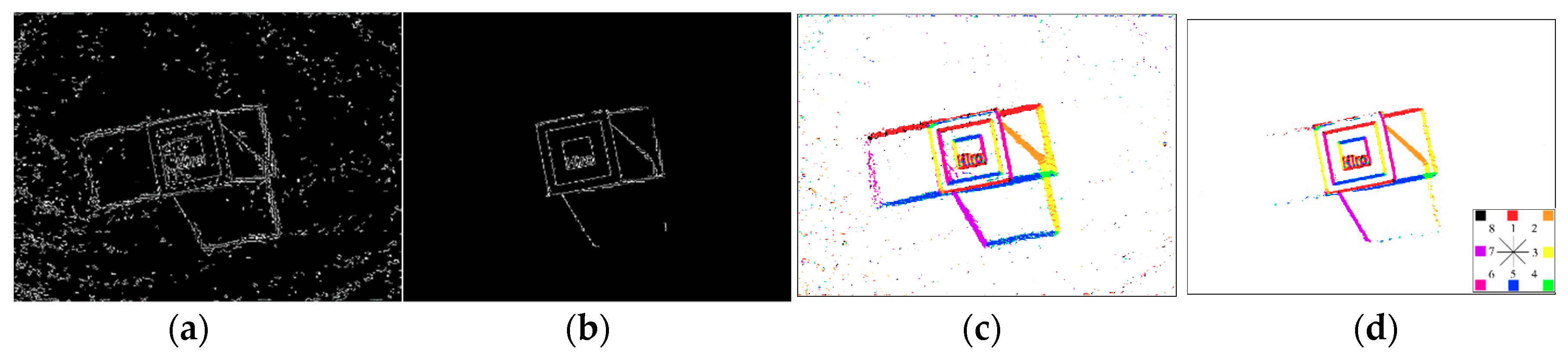Figure 3a,b show the results of Figure 2 obtained using the Canny edge detector with two double threshold intensity values of 10 and 20, and 20 and 40, respectively. Previous shadow detection methods based on the shadow edges have generally assumed that accurate edges are detected in the image [18]. However, it is difficult to determine the proper threshold values for detecting the shadow edges. Figure 3c,d show the gradient direction distribution obtained using the Sobel operator (3 by 3 mask). Here, only points with gradient magnitudes higher than two threshold values (10 and 20 for Figure 3c,d, respectively) are represented. The gradient direction is coded to eight directions, which are marked by eight different colors (see inset in Figure 3d).

2.2. Gradient-Based Shadow Boundary Detection

After converting a given RGB input image to a YUV image, we apply a Sobel mask to the Y image, and then compute the gradient information (i.e., the magnitude and direction). Our method examines whether the gradient direction of each pixel in the image is the same as the normal direction of the shadow boundary line of the candidate light source. Only pixels with the same direction as the candidate shadow boundary are classified as matched points, within eight gradient direction ranges. Since the 3-D AR marker is a cubic object, the shadow map generated by the candidate light source consists of four or five shadow line segments. This examination is therefore repeated for every line segment making up the candidate shadow.

At points where the gradient direction check passes, the non-maximum suppression, based on the gradient direction, is employed to remove spurious matching pixels. The gradient magnitude value of the anchor (center) pixel in a local mask (3 by 3) is compared with the gradient magnitudes of the two neighbor pixels along the same gradient direction. In other words, we check whether or not three consecutive pixels, including the center pixel of the mask, have the same gradient direction. Then, if the center pixel has a higher gradient magnitude value than the neighboring pixels on both sides, we determine the center pixel to have passed the non-maximum suppression.

To confirm that the candidate shadows are actually present in the image, we then perform gradient-based matching along the candidate shadow boundary. Along the boundary line segment of the candidate shadow, 10 pixels are sampled at regular intervals, considering the length of the line segment.

The distance between the upper corner point of the 3-D marker and the cast point on the shadow surface changes according to the incline angle of the candidate light source. This means that the shadow boundary corresponding to the edge of the upper plane of the 3-D marker may be blurred in the image. Therefore, in our method we examine more neighboring pixels along the gradient direction (perpendicular to the boundary line) to detect the soft-edged shadow. The distance from the corner of the 3-D AR marker to the corresponding vertex of the shadow boundary can then be calculated. For the soft edge connecting the two upper corners, we compute the average distance of the two upper corners, and one tenth of this distance is used as the width of the region of interest. Here, we sample 10 points in a vertically bi-directional direction, with respect to the boundary line, for gradient-based matching. In general, vertical shadow boundaries originate from the bottom corners of the AR cube marker. In this case, as the bottom corner is attached to the shadow surface, and the distance from this vertex is zero. We therefore compute the distance from the other vertex that constitutes the vertical boundary (the upper corner), to its projection point on the shadow surface. Our algorithm divides this distance by two, and uses this as the width of the sampling region.

2.3. Line Fitting and Matching Score Computation

Line fitting is performed using only the points that have passed the gradient direction matching, as described in Section 2.1. We use principal component analysis (PCA) to obtain the normal (direction) information of the fitted line [19]. If an insufficient number of points have passed the gradient direction matching, we determine that a reliable shadow boundary is not detected (under 20 pixels, experimentally).

When the shadow cast by the i-th candidate light source has N line segments, we compute the matching score, L_{i_k}, on the k-th line segment, as shown in Equation (1):

$$L_{i\_k}=1-e^{-\frac{r_{i\_k}}{{\tau }_1}},C_{i\_1}=\frac{1}{N}{\displaystyle \sum _{k=1}^n{L}_{i\_k}},$$

(1)

where r_{i_k} represents how many pixels in the image are matched with the i-th candidate’s shadow boundary elements; r_{i_k} is computed by dividing the number of the matched points by the total number of the sample points on k-th line segment. N is the total number of shadow boundary lines cast by the i-th candidate light source, τ_{_1} is used to control the relative influence of the gradient direction matching (here it is set to 0.3, experimentally), and C_{i_1} is the average score of the gradient-based matching of the i-th candidate light source. This measure represents the number of points that support the shadow boundary cast by the i-th candidate light source.

We compute an angular difference between the candidate shadow boundary line and the fitted line using the matched points. Specifically, we compute a slope direction, θ_{A_ik}, of the k-th boundary line of the i-th shadow, and a slope direction, (θ_{B_ik}), of the fitted line segment, respectively. We can then obtain the angular difference, D_{i_k}, using Equation (2) (τ_{_2} is set to 3, experimentally). Here, C_{i_2} is the average score of the angular difference of the i-th candidate light source in the image.

$$\begin{array}{c}{D}_{i\_k}=e^{-\frac{\Delta {Angle}_{i\_k}}{{\tau }_2}},C_{i\_2}=\frac{1}{N}{\displaystyle \sum _{k=1}^n{D}_{i\_k}},\\ \Delta {Angle}_{i\_k}=\min ({180}^{\circ }-\left|{\theta }_{A\_ik}-{\theta }_{B\_ik}\right|,\left|{\theta }_{A\_ik}-{\theta }_{B\_ik}\right|)\end{array}$$

(2)

When the AR marker occludes the i-th light source, we can compute the position of the upper corner of the AR marker on the shadow surface, which is a vertex of the shadow boundary. Our algorithm computes a distance score, E_{i_k}, between the intersection point of the fitted line and the projected corner point of the AR marker. The cubic marker is employed, meaning that the number of intersection points is one less than the total number of the shadow boundary lines. This measure represents how close the junction of the shadow boundary is to the projected upper corner of the 3-D marker on the shadow surface. E_{i_k} is calculated as follows:

$$E_{i\_k}=e^{-\frac{{\mathit{error}}_{i\_k}}{{\tau }_3}},C_{i\_3}=\frac{1}{N}{\displaystyle \sum _{k=1}^n{E}_{i\_k}},{\mathit{error}}_{i\_k}=\Vert {\mathit{projPt}}_{\mathit{ik}}-{\mathit{fittingPt}}_{\mathit{ik}}\Vert ,$$

(3)

where projPt_ij is the j-th projected corner position of the i-th candidate shadow, and fittingPt_ij is the intersection between the (j − 1)-th shadow boundary and the j-th shadow boundary. Here, τ_{_3} is set to 8, experimentally.

Figure 4a shows one of the shadow boundaries of the candidate illumination source. The upper and lower corners are represented by red and yellow, respectively. Figure 4b shows the matched (red) points in the search region of the third shadow boundary line segment. A total of 100 points in the search region are sampled, along 10 line segments. Each of these sections has the same slope as the boundary line, in a vertically bi-directional direction with respect to the boundary line (Figure 4b). Figure 4c shows the fitted boundary lines (green) with the matched points and their intersection points (purple). The corners (cyan) are also shown, consisting of the bottom plane of the AR marker and the cast points (yellow) of the top plane.

For the candidate shadow cast by the i-th candidate light source, the final matching score is given by a weighted sum of the three components shown in Equation (4). The score conveys how much of the candidate shadow boundary is actually extracted from the image. Here ω₁, ω₂, and ω₃ are used to control the relative influence of three terms, which are set to 0.6, 0.2, and 0.2, respectively.

$${\mathit{Cost}}_i={\omega }_1\cdot C_{i\_1}+{\omega }_2\cdot C_{i\_2}+{\omega }_3\cdot C_{i\_3}$$

(4)

As the position of the i-th candidate light source is denoted by its longitude and latitude, the final matching score can be represented using either a geographic or a spherical coordinate system. We assume that the environmental illumination source is a point light, but real light sources generally have a constant volume. In order to consider light sources with some area in the real scene, such as a light bulb, we apply Gaussian smoothing (3 by 3) to the final matching score map, which we represent here using longitude and latitude.

2.4. Verification of Local Feature-Based Matching

We follow our local feature-based examination with a verification procedure, to more precisely estimate the environmental illumination. In this study, we employ a low threshold value in the local feature-based examination, to avoid missing the important illumination sources. We found that using this low threshold means that candidate shadows passed by the local feature examination overlap each other significantly. In this case, the shadow map created by the passed illumination source is contained in those of the other light sources. The relative brightness of the shadow regions illuminated by more light sources becomes darker. By using the intersection sets of the passed shadow regions and their difference sets, we can compute the relative extent to which the shadow areas are darkened, considering the inclusion relationships between the different illumination sources.

In Equation (5), S_n represents the n-th candidate shadow region created by the n-th illumination source, and S_nm represents the intersection region of the n-th shadow and the m-th shadow. S’_n represents the n-th shadow region, except for the areas that overlap with other shadows. S’_n is computed by subtracting M from S_n; M is the unified region of the intersection of the candidate shadows. S’_mn represents the pure intersection region of the n-th shadow and the m-th shadow, excluding the overlapping regions with another shadow, and N is the total number of candidate shadows. M is calculated as follows:

$$M={\displaystyle \underset{n=1}{\overset{N-1}{\cup }}{\displaystyle \underset{m=n+1}{\overset{N}{\cup }}(S_n{\displaystyle \cap S_m})}},{S\text{'}}_{nm}=S_n{{\displaystyle \cap S}}_m-{\displaystyle \underset{n=1,k\ne n,m}{\overset{N}{\cup }}(S_n{{\displaystyle \cap S}}_k}).$$

(5)

In Figure 5, four shadow maps (S₁ to S₄, denoted as (c), (d), (e), and (f), respectively) are generated by the local feature-based matching, and the S₄ region with the lowest matching score is contained in S₂. Here, the subscripts of the shadow maps are numbered in descending order of their matching scores. Figure 5g shows the M region of the four shadow maps, and Figure 5h shows region S’₄ (red) within region S’₂ (yellow). We examine whether region S’₄ becomes sufficiently darker than region S’₂ in the input image. Figure 5a shows that there is little difference in brightness between regions S’₄ and S’₂ in Figure 5h (red and yellow, respectively). Since the fourth candidate illumination source with the lowest matching score does not render a shadow region sufficiently dark, the fourth illumination source is removed. Among the candidate shadows passed by the local feature examination, our verification procedure can precisely choose the candidate shadow sets that best represent the real shadows in the image. Previous methods have been unable to examine the case of the overlapping casted shadows in scenarios where there are lights with the same azimuth and different elevation angles in the hemisphere [18]. Our proposed verification procedures, however, enable the problem of overlapping casted shadows in the scene to be solved.

3. Results

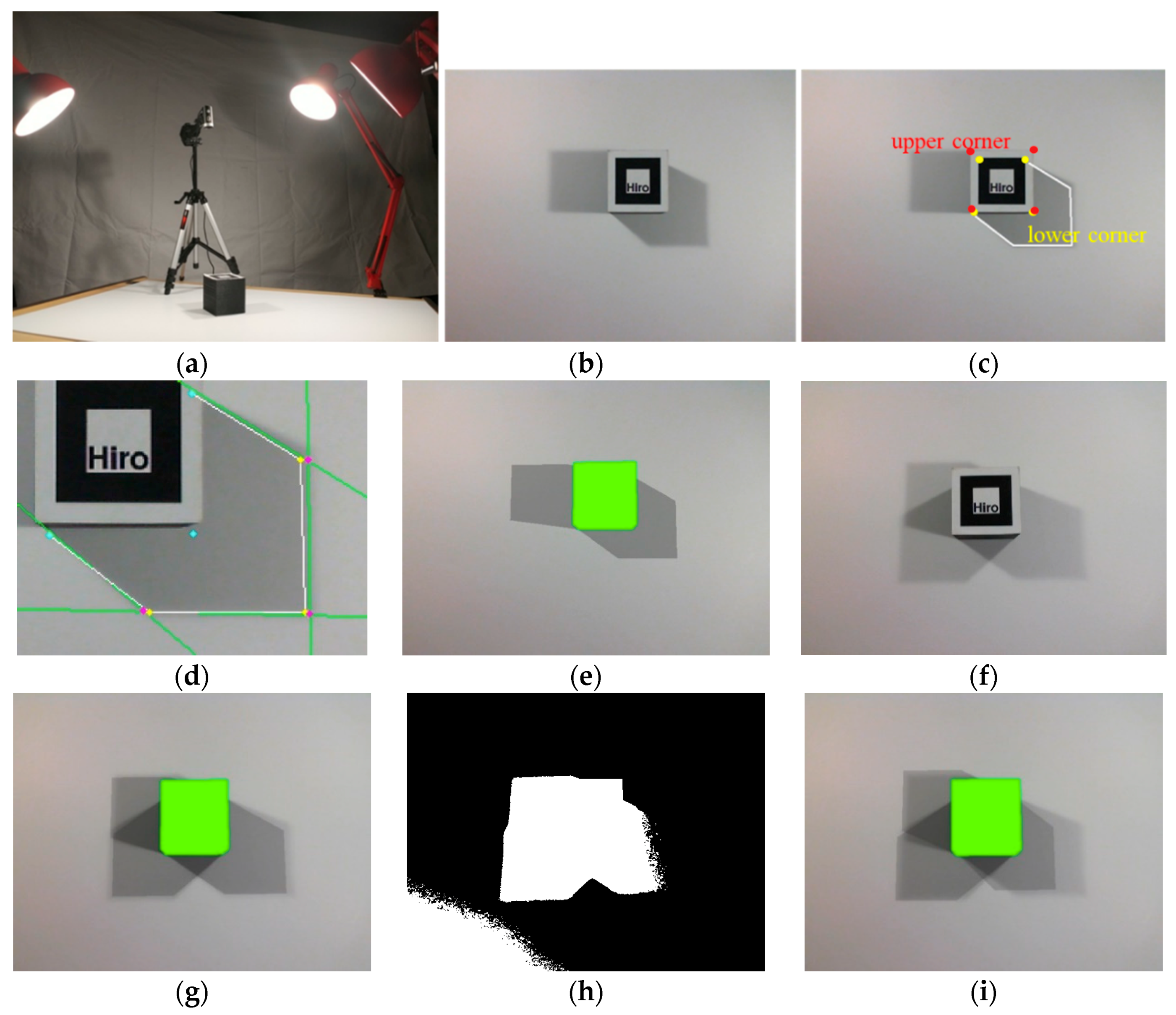
The experimental equipment consisted of a PC with 3.4 GHz CPU. Figure 6a shows the experimental setup used to estimate the environmental illumination distribution. We manually measured the directions of real light sources (in the elevation angle, θ, and the azimuth angle, φ, in the spherical coordinate system), using the marker’s center to ground truth. In this experiment, we used two to three bulbs (each 5 cm in diameter) as the environmental light sources.

The candidate shadow consists of four to five boundary line segments. The image features (gradient direction and magnitude) are examined along the shadow line segments that make up the candidate shadow boundary. Specifically, we examined to what extent the shadows cast by the top plane and the side walls of the 3-D marker correlate with the image features on the shadow surface. Figure 6b,f show the input image with two and three illumination sources, respectively. Figure 6d shows the shadow boundaries and intersection points of the detected shadow lines, and Figure 6e,g show the final rendered image, estimated with two and three illumination sources, respectively, using the proposed method. Figure 6h,i show the threshold image (by 150 intensity value) and the rendered image, made using a previously published method [4]. Figure 6h shows that the threshold value selection greatly affects the region-based shadow region detection. This indicates that the previous illumination estimation methods based on shadow detection are dependent on the illumination condition. In the point-based approaches, careful sampling is necessary to produce variation in the distribution of these light sources that is to be maximized. For example, the method of Sato et al. sometimes fails to provide a correct estimate of the illumination distribution because it is sensitive to the number of sampling points and their positions [1]. To compare our proposed method with the method previously published in Reference [4], we overlaid the rendered shadows onto the input shadow image. The previous method examines the ratio between the threshold shadow image regions and the candidate shadow mask regions created by the illumination sources. The performance of the previous method is therefore heavily dependent on the determination of the threshold value for the shadow region segmentation. The real shadow region in Figure 6h is not sufficiently detected, meaning that the illumination information for the shadow region is incorrectly estimated.

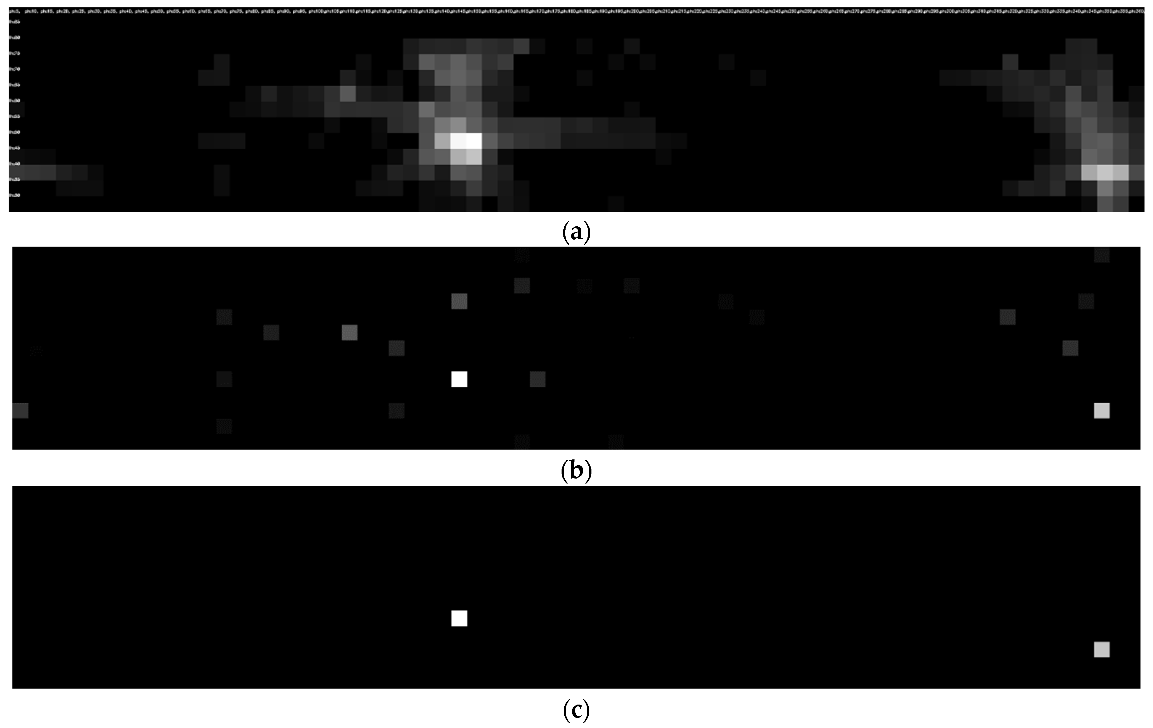
The candidate shadows are generated at 5° intervals in both the azimuth angle (0–360°) and the elevation angle (30–85°). The total number of candidate shadows is 864 (72 × 12), and the matching scores of the candidate shadows are represented in the 2-D domain. Figure 7 shows the illumination source distribution for the scene depicted in Figure 6b. High-intensity illumination sources usually generate a shadow region with distinct edges. Therefore, the highest score is obtained at the angular position where the illumination source with the highest intensity is located. Because the order of the matching score generally coincides with the order of the illumination intensity, we represented the matching scores of another illumination source relative to the highest matching score, as shown in Figure 7a. In this experiment, we used a bulb with a diameter of 5 cm, covering one sample area in the longitude and latitude domains. Assuming that the two illumination sources are not attached to each other, we employed Gaussian smoothing and non-maximum suppression in a 3 by 3 mask to remove the spurious neighbor matches, as shown in Figure 7b. The final illumination positions were determined using the weighted average of the matching costs in the 3 by 3 mask, of which the center pixel is the local maximum position for the non-maximum suppression.

In the experimental results, we found that illumination sources with matching scores <35% relative to the brightest illumination source could be classified as insignificant. However, by using this low threshold value, we may also detect false shadows, meaning that an illumination source casting an indistinct shadow may incorrectly be classified as an important source in the scene. To verify these potentially falsely-detected illumination sources, we calculated the intersection sets of the shadow regions that passed the local feature-based matching. By computing the relative extent to which these shadow areas were darkened according to the inclusion relationships of the candidate shadows, we were able determine the important illumination sources from the passed shadow regions.

To evaluate the performance of the proposed method, we estimated the illumination information for two cases: one with two light sources and one with three.

Table 1. Comparison of the measured and estimated light directions.

				Light 1	Light 2	Light 3	Average Absolute Deviation
Two illumination sources	Case 1	Measured	Elevation	46.3°	40.3°		-
			Azimuth	148.0°	349.0°		-
		Proposed method	Elevation	49.1°	39.8°		1.65°
			Azimuth	146.5°	350.5°		1.50°
		Previous method	Elevation	50.0°	40.0°		2.00°
			Azimuth	145.0°	350.0°		2.00°
	Case 2	Measured	Elevation	63.1°	57.3°		-
			Azimuth	81.0°	316.0°		-
		Proposed method	Elevation	64.0°	58.6°		1.10°
			Azimuth	81.0°	320.7°		2.35°
		Previous method	Elevation	60.0°	55.0°		2.70°
			Azimuth	75.0°	320.0°		5.00°
Three illumination sources	Case 3	Measured	Elevation	39.4°	40.3°	41.2°	-
			Azimuth	206.0°	154.0°	26.0°	-
		Proposed method	Elevation	41.2°	40.5°	41.6°	0.80°
			Azimuth	206.2°	154.3°	26.1°	0.20°
		Previous method	Elevation	40.0°	35.0°	55.0°	6.57°
			Azimuth	210.0°	155.0°	35.0°	4.67°
	Case 4	Measured	Elevation	41.3°	38.4°	45.6°	-
			Azimuth	35.0°	154.0°	340.0°	-
		Proposed method	Elevation	43.6°	40.9°	46.3°	1.83°
			Azimuth	36.4°	149.0°	341.2°	2.53°
		Previous method	Elevation	40.0°	50.0°	45.0°	4.50°
			Azimuth	35.0°	140.0°	335.0°	6.33°
	Case 5	Measured	Elevation	33.9°	30.0°	37.0°	-
			Azimuth	20.0°	140.0°	200.0°	-
		Proposed method	Elevation	35.0°	32.0°	38.6°	1.57°
			Azimuth	18.5°	143.6°	193.8°	3.77°
		Previous method	Elevation	60.0°	30.0°	35.0°	9.37°
			Azimuth	30.0°	145.0°	195.0°	6.67°

shows the comparison of the results of the existing method and those of the proposed method. More specifically, the errors of the obtained illumination sources were computed using the average absolute deviation of the measured angles and the computed angles. Table 1 shows that the light directions estimated by the proposed method are closer to the ground truths (measured directions) of the real light sources, as compared to results generated by the method previously published in Reference [4]. Figure 6b shows the input image from Case 1 of Table 1. Figure 8 shows the input images of Cases 2 to 5, and the final AR image of the Utah teapot model in Case 4. Figure 8e,f show the comparison of the effects of the illumination locations obtained by the previous method to those obtained by the proposed method. To generate images that are more naturally rendered, 15 subsampling points per the obtained illumination source were generated. In comparison the real scene (Figure 8c), we can see that the shadows obtained by the previous method are generated falsely.

Table 2. Computation time (ms) of modules.

AR Marker Recognition	Candidate Shadow Generation	Image Gradient Computation	Gradient-Based Matching	Non-Maximum Suppression	Local Feature-Based Matching	Total
8.5	15.0	10.6	42.0	1.0	11.6	88.7

shows the modular computation performance. Initially, the AR marker was recognized and candidate shadow maps were generated. The image gradient-based matching procedure including color converting, Gaussian smoothing, and Sobel operations (gradient and magnitude computation) was performed. The gradient-based matching procedure, consisting of line fitting and junction point evaluation, took almost half the total calculation time. The local feature-based matching was performed when the shadows overlapped. Otherwise, this final module did not need to be performed. The proposed method generated the final rendering image in about 77.1–88.7 ms (11.3–13.0 frames/s). In general, since the change of the environmental illumination distribution does not happen in every frame, the proposed method can be applied to real-time applications. To further improve the performance, we will consider a parallel implementation in Compute Unified Device Architecture (CUDA), thus offering greater computation efficiency, in the near future.

The proposed method assumes that the distance to the light source was constant. In this experiment, the radius of the hemisphere with the candidate light source was set to 2 m. To estimate the illumination information in a dynamic environment (one in which the light sources are moving), we will consider the illumination environment of a 3-D space instead of a hemisphere in the near future.

Our proposed method can reduce the unwanted effects caused by the threshold values during edge-based shadow detection, in addition to those caused by the sampling position during point-based illumination estimation. Our proposed method was tested on an untextured shadow surface, but it can also be applied for the detection of shadows on textured shadow surfaces by using the illumination invariant conversion [2,5]. The proposed method is applicable for model-based line segment detection in the image, with non-salient and cluttered gradient distribution. In further studies, we will consider the case where there are area light sources of a certain size, such as incandescent lamps, in the scene. We will include the shading technique for more realistic images in augmented reality according to changing environment illumination.

4. Conclusions

By using the shadow casting information of the 3-D AR marker from the candidate light source, we can extract the shadow boundary from the image. In more detail, the proposed method measures the edge support, which indicates that the image gradient has the same direction as the cast shadow boundary. We computed the angular difference of the fitted line segments and the candidate shadow boundary, and we computed the corner support that represents the distance between the intersection point of the fitted line segments and the corner point of the 3-D marker that is casting the shadow. To verify any falsely-detected illumination sources in the local feature-based matching, we computed the inclusion relationships between the different shadow regions, and examined the relative extent to which the shadow areas are darkened.

Since the proposed method involves model-based line segment detection in the image, the unwanted effects caused by the threshold values during edge-based shadow detection can be reduced. Also, since the proposed method employs area-based candidate shadow maps in the shadow region verification, the problems caused by the sampling position during point-based illumination estimation can be alleviated. In the near future, we will consider parallel implementation in CUDA with computation efficiency to improve the performance of the proposed method. To cope with a dynamic illumination environment (moving light sources), we will consider the illumination environment of a 3-D space instead of a hemisphere.